Multi-Attribute Decision-Making Using Hesitant Fuzzy Dombi–Archimedean Weighted Aggregation Operators

Peide Liu; Abhijit Saha; Debjit Dutta; Samarjit Kar

doi:10.2991/ijcis.d.201215.003

<Previous Article In Issue

Download article (PDF)

Next Article In Issue>

Volume 14, Issue 1, 2021, Pages 386 - 411

Multi-Attribute Decision-Making Using Hesitant Fuzzy Dombi–Archimedean Weighted Aggregation Operators

Authors

Peide Liu¹^{, *}^,, Abhijit Saha², Debjit Dutta³, Samarjit Kar⁴

¹School of Management Science and Engineering, Shandong University of Finance and Economics, Jinan Shandong, 250014, China

²Faculty of Mathematics, Techno College of Engineering Agartala, Tripura, 799004, India

³Faculty of Basic and Applied Science, NIT Arunachal Pradesh, Arunachal Pradesh, 791112, India

⁴Faculty of Mathematics, NIT Durgapur, West Bengal, 713209, India

^*Corresponding author. Email: peide.liu@gmail.com

Corresponding Author

Peide Liu

Received 7 September 2020, Accepted 11 December 2020, Available Online 22 December 2020.

DOI: 10.2991/ijcis.d.201215.003 How to use a DOI?
Keywords: Hesitant fuzzy set; Archimedean t-norm and t-conorm; Dombi t-norm and t-conorm; Dombi–Archimedean weighted aggregation operators; multi-attribute decision-making
Abstract: Multi-attribute decision-making (MADM) has been receiving great attention in recent years due to two major issues which are basically to describe attribute values and secondly to aggregate the described information to generate a ranking of alternatives. For the first case it entails the hesitant fuzzy elements (HFEs) as a more flexible and general tool in comparison to fuzzy set theory and for the second one, we allow the aggregation operator (AO) as an effective tool. Having said that there is not yet reported an AO which can provide desirable generality and flexibility in aggregating attribute values under hesitant fuzzy (HF) environment, although many AOs have been developed earlier to attempt to meet above such eventualities. So, the primary objective of this paper is to develop some general as well as flexible AOs that can be exploited to solve MADM problems with the HF information. From this perspective, at the very beginning, we develop some operations between HFEs by uniting the features of Dombi and Archimedean operations. Next, we bring up some HF weighted AOs based on Dombi and Archimedean operations. We discuss in detail some intriguing properties of the proposed AOs. Secondly, we emphasize establishing a procedure of MADM endowed by the proposed operators under the HF environment. Finally, we present a practical example concerning human resource selection to gloss the decision steps of the proposed method and at the same time, we explore the feasibility of the new method.
Copyright: © 2021 The Authors. Published by Atlantis Press B.V.
Open Access: This is an open access article distributed under the CC BY-NC 4.0 license (http://creativecommons.org/licenses/by-nc/4.0/).

1. INTRODUCTION

In most of the real-life decision circumstances, the prevalence of multi-attribute decision-making (MADM) problems is vividly known. The primary objective of the MADM approach is to determine the best-suited alternative(s) from a set of available alternatives with respect to multiple attributes, both qualitative and quantitative. It has been observed the significant success rate of many MADM approaches in the case of web 2.0 [1], social network [2], and recommendation system [3,4]. Various regulating factors viz. a shortfall of information and consciousness, hardness in information expulsion, incertitude of the decision-making ambiance, etc. will come in limelight especially in many real-world situations on account of the rising perplexity of the socio-economic conditions. As a result, for decision-makers, it comes true a formidable task to unveil numerically to the values of attributes. In lieu, representation of the preferences using fuzzy numbers or extended fuzzy numbers [5–8] is more appropriate indeed.

For the last few years, it has been noticed about the extensive theoretical study of numerous MADM problems. The various approaches about MADM have been put forward in the framework of the fuzzy set (FS) theory [9–13]. The notion of the hesitant fuzzy set (HFS) that was first reported by Torra [14] is reckoned as an extension of the FS which allows the membership grades presuming a set of possible values instead of a single one. In case of dealing the fuzzy uncertain information, such HFS can contribute as a strong tool. The connection between the HFS and other extended FSs were investigated by Torra and Narukawa [15] in which an intuitionistic fuzzy set (IFS) is appeared to be an envelope of HFS and all possible HFSs are lying in the category of the type-2 fuzzy set (T2FS). Xu and Xia [16] suggested a class of distance and similarity measures for HFS and subsequently, they proposed further the hesitant ordered weighted distance measures and the hesitant ordered weighted similarity measures. The concept of generalized hesitant fuzzy synergetic weighted distance (GHFSWD) measure and also, some obligate properties along with their feasible applications was studied by Peng et al. [17]. The strong connection among similarity measure and distance measure for HFS, the interval-valued hesitant fuzzy set (IVHFS), and entropy was reported by Farhadinia [18]. Qian et al. [19] were able to explore HFS through IFS and utilized it in the decision support system. Chen et al. [20] exercised interval-valued hesitant preference relations and successfully applied it to group decision-making problems. The idea of the dual hesitant fuzzy set (DHFS) was put forth by Zhu et al. [21]. Rodríguez et al. [22] brought the notion of hesitant fuzzy (HF) linguistic term set which explaining the supremacy of linguistic excerption with the help of a fuzzy linguistic approach. The forcible VIKOR method can be utilized to solve a series of MADM problems having HF information which was propounded by Zhang and Wei [23]. We note that Zhang and Xu [24] expanded the tools of TODIM to adapt the HF environment and they were able to provide two HF decision-making approaches. Dong et al. [25] formulated the efficient consensus model adopting hesitant linguistic assessments in group decision-making. For HF linguistic preference relations, Zhu and Xu [26] yield some compatibility measures. In succession, Wang and Xu [27] presented in their study, the idea of extensive HF linguistic preference relations. It has been observed the widespread of the HFS and some varieties in its extension especially in the fields of group decision-making [28–34] preference relations [35], clustering analysis [36], and other applications [37–40]. Aiming at transparent aspects of the varied ideas, tools, and affinities in connection with the extent of FS, lately, Rodríguez et al. [41] summarized the HFSs. Over and above, Xu [42] devoted toward review in detail about the progress of aggregation techniques and infliction for HFS and side by side indicated several active trends in this domain.

We note that although in general, Aggregation operators (AOs) are considered just as functions mathematically but confronting as very common techniques, these suffice to integrate all the input individual data into a single one. Over the last three decades, both researchers and practitioners have been giving attention toward inquisition on AOs on account of their large impact in the vicinity of wide ranges of information processing, such as decision-making, pattern recognition, information retrieval, medical diagnosis, data mining, machine learning, etc. We may recall here that the study of HF AOs has been drawing significant attention to the researchers due to its importance for information fusion. Xia and Xu [43] provided a series of AOs and developed their enviable features. In this context, we also mention here that Xia et al. [44] employed quasi-arithmetic means to constitute several series AOs in the regime of HF environment. Wei [45] proposed some preference operators and used them to deal with MADM problems where the attributes perform various levels of priority under a HF environment. Furthermore, many hesitant interval-valued AOs were put forth by Wei et al. [46], and even they developed a procedure to solve interval-valued hesitant fuzzy MADM problems. Having paid heed to all the ideas of fuzzy integral theory, Wei et al. [47] attempted to utilize the Choquet integral to have two AOs adhering to the HF information: hesitant fuzzy Choquet ordered averaging (HFCOA) operator and hesitant fuzzy Choquet ordered geometric (HFCOG) operator. In this context, it may be pointed out that these two aforementioned operators are not only taken it granted based on the importance of attributes but also another aspect of its consideration is solely due to an active role in determining the correlations among the independent attributes. It was possible to solve MADM problems by applying both the HF Bonferroni mean, introduced by Zhu et al. [48] and geometric Bonferroni mean. To aggregate HF information, Zhang [49] interpreted a large extent of HF power AOs and in turn, examined different fascinating properties and relationships among those operators. Zhang and Wu [50] suggested two weighted HF AOs invoking the Archimedean t-conorms and t-norms, leading to aggregate weighted HF information. Zhang et al. [51] considered some induced generalized HF operators and utilized them to MADM problems. It was Liao and Xu [52] who lead a significant contribution for searching some HF hybrid weighted AOs and at the same time formed a decision algorithm to assist MADM problems utilizing HF information. Surprisingly, Zhou and Xu [53] put forward two new aggregation approaches-first one is an optimal discrete fitting AO and the second one is, simplified optimal discrete fitting AO to analyze group decision-making problems. In the meantime, two AOs for hesitant fuzzy linguistic term set (HFLTS) were defined by Wei et al. [54] which are respectively the HFLWA (Hesitant fuzzy linguistic weighted aggregation) operator and the HFLOWA (Hesitant fuzzy linguistic ordered weighted aggregation) operator and on the other hand, utilized these operators to solve MADM problems based on the conditions in which importance weights of criteria or experts are known or unknown. Based on Einstein's operational laws, Yu [55] established a few more HF AOs. Some special kinds of operators called HF Hamacher AOs were introduced by Tan et al. [56] for handling the MADM problems. It is equally important to mention here that Qin et al. [57] with their work stimulated the idea by presenting some new HF operators associating the Maclaurin symmetric mean and also considered a variety of allied eligible properties. We recall that upon a state of being more or less with HF Bonferroni mean operators [58], the notable characteristics of HF Maclaurin symmetric mean is that it can record the entire interrelationships between the arguments; hence it is more usual and appropriate for serving the real-world decision-making problems. We also refer here that it is possible to determine new some HF AOs using Frank operations which exclusively achieved by Qin et al. [59] together with solving the MADM problems. Liao and Xu [60] developed a VIKOR method for solving MADM under HF environment. The notion of the cubic HFS was developed by Mahmood et al. [61] to deal with MCDM problems. He [62] successfully carried out the operations of Dombi operators to Typhoon disaster assessment under a HF environment. Xu and Zhou [63] implemented hesitant probabilistic fuzzy operations and used them to solve group decision-making problems. In this context, it may be pointed out that as an augmentation of the hesitant probabilistic fuzzy weighted averaging operator and hesitant probabilistic fuzzy weighted geometric operator, Park et al. [64] made their remarkable contribution by introducing hesitant probabilistic fuzzy Einstein weighted averaging operator and hesitant probabilistic fuzzy Einstein weighted geometric operator respectively. It is worthy to say that various theoretical and practical reasoning can be simplified with the help of a uniformly typical hesitant fuzzy set (UTHFS) which was articulated by Alcantud and Torra [65]. Fairly recently, Wang and Li [66] introduced operational laws of picture hesitant fuzzy elements (PHFEs) and attributed them to define generalized picture HF AOs which genuinely helped to tackle the varied situations while we cope up with MCDM in the framework of picture HF environment. Interestingly, an improved A* algorithm based on hesitant FS theory for multi-criteria Arctic Route planning was developed by Wang et al. [67]. We do refer here that Lioa et al. [68] practiced HF linguistic preference utility set in the selection process of fire rescue plans. To serve the personnel selection problem, Yalcin and Pehlivan [69] were able to construct a methodology in which the fuzzy CODAS method gets connected with the fuzzy envelope of HFLTSs concerning the comparative linguistic expressions. Moreover, Wu et al. [70] formulated a unique dynamic emergency decision-making method with probabilistic HF information underlying the GM (1, 1) model for prophecy of the decision-making information at the subsequent stage. Alcantud et al. [71] first reported the notion of dual extended HFSs and even employed them to develop an algorithm that involves a weight score function. Furthermore, Liu et al. [72] initiated the HF cognitive maps and showed how to use it for the exploration of the risk factors that arise in an electric power system. Exploiting the regret theory, Liu et al. [73] submitted an approach for probabilistic HF MADM in view of the selection process of venture capital investment projects.

The Dombi operations, after the name of Dombi [74] are nothing but the operations of t-norm and t-conorm, bearing the nature of good flexibility with the general parameter. On the contrary, Archimedean t-norms and t-conorms [75–77] are the generalizations of many other t-norms and t-corms like algebraic t-norm and t-conorm, Einstein t-norm and t-conorm, Hamacher t-norm and t-corm, etc. The operations of Archimedean t-norms and t-conorms are treated as Archimedean operations. The growing capacity of decision complexity induces the real-life decision-making problems that indulge both generality of the operations used and flexibility of the parameters that appeared. In this context, it is more appropriate to suggest a tool obtained through merging the Dombi and Archimedean operations to serve the purpose. Due to different characteristics, AOs obtained through Archimedean operations will not generate the same ranking order deduced from Dombi operations based AOs. Thus, optimal alternative(s) may not be the same in these two cases. Since the fusion of Dombi and Archimedean operations will retain their individual characteristics, so it is logical to combine them for the purpose of aggregation. As far as we know, no such study has been carried out related to AOs based on the simultaneous act of the Dombi and Archimedean operations when we deal with the HF decision-making problems. Getting inspired and provoked by that fact, in this paper, we have tried to investigate a family of AOs with the coalescence of Dombi operations and Archimedean operations that regard HF information and successfully conjoin them to solve MADM problems. The aims in this article are pursued below:

Suggest some operational laws and AOs under HF environment with the help of the simultaneous act of Dombi and Archimedean operations.
Construct a novel MADM method with HF information based on the proposed AOs and illustrate it with a numerical example.

In such scenarios, we propose in this study, some Dombi–Archimedean operational laws for hesitant fuzzy elements (HFEs) alongside some HF Dombi–Archimedean AOs, such as hesitant fuzzy Dombi–Archimedean weighted arithmetic aggregation operator (HFDAWAA), hesitant fuzzy Dombi–Archimedean ordered weighted arithmetic aggregation operator (HFDAOWAA), hesitant fuzzy Dombi–Archimedean hybrid arithmetic aggregation operator (HFDAHAA), hesitant fuzzy Dombi–Archimedean weighted geometric aggregation operator (HFDAWGA), hesitant fuzzy Dombi–Archimedean ordered weighted geometric aggregation operator (HFDAOWGA), hesitant fuzzy Dombi–Archimedean hybrid geometric aggregation operator (HFDAHGA). In addition to this, we require to initiate a procedure for the MADM approach after interposed by the proposed AOs in the regime of HF environment.

We summarize the rest part of this paper as follows. In Section 2, we introduce in brief some important and vital concepts of HFSs, Archimedean t-norm (t-conorm) and Dombi t-norm (t-conorm). In Section 3, we define the Dombi–Archimedean operational laws for HFEs. In Sections 4, we develop some HF Dombi–Archimedean AOs, such as HFDAWAA, HFDAOWAA, HFDAHAA, HFDAWGA, HFDAOWGA, and HFDAHGA. All the essential properties of these operators are also demonstrated. In Section 5, we present a novel approach using the proposed AOs beneficial for stirring the various kinds of MADM problems in which the attribute values take the form of HF information. In Section 6, we allow an example of personnel selection to gloss the proposed method. Section 7 is solely devoted to a comparative study to confirm the superiority of the proposed method. In the end, in Section 8, we make some conclusions upon this entire study.

2. PRELIMINARIES

In this section, we briefly review some basic concepts of HFS, Archimedean and Dombi operations, which will be directly used in the next sections.

2.1. Hesitant Fuzzy Sets

Definition 1.

[14] Let U be a finite universe of discourse. Then a HFS ξ on U is defined as:

ξ=<x,μξh(x)>:x∈U

where μξh:U→2[0,1] is a mapping and μξh(x) denotes the set (finite) of possible membership degrees of the element x∈U.

Given x∈U, μξh is termed as a HFE [43]. For sake of simplicity, the HFS ξ is represented by 〈μξh〉. The set of all HFEs on U is denoted by HFEU.

Definition 2.

[43] For two HFEs μξ1h and μξ2h on U, some basic operations between them can be described as:

μξ1h∪μξ2h=∪α1∈μξ1h,α2∈μξ2hmax{α1,α2}
μξ1h∩μξ2h=∪α1∈μξ1h,α2∈μξ2hmin{α1,α2}
μξ1hc=∪α1∈μξ1h{1−α1}
μξ1h⊕μξ2h=∪α1∈μξ1h,α2∈μξ2hα1+α2−α1α2
μξ1h⊗μξ2h=∪α1∈μξ1h,α2∈μξ2h{α1α2}
λμξ1h=∪α1∈μξ1h1−(1−α1)λ (λ>0)
μξ1hλ=∪α1∈μξ1h(α1)λ (λ>0)

Theorem 1.

[43] Let μξ1h and μξ2h be two HFEs defined on U and λ,λ1, λ2>0. Then

μξ1h⊕μξ2h=μξ2h⊕μξ1h
μξ1h⊗μξ2h=μξ2h⊗μξ1h
λμξ1h⊕μξ2h=λμξ1h⊕λμξ2h
μξ1h⊗μξ2hλ=μξ1hλ⊗μξ2hλ
λ1+λ2μξ1h=λ1μξ1h⊕λ2μξ1h
μξ1hλ1+ λ2=μξ1hλ1⊗μξ1hλ2

Definition 3.

[43] Let μξh be a HFE on U. Then the score value of μξh is defined as:

Sμξh=1#μξh∑α∈μξhα

where #μξh denotes the number of elements in μξh.

Based on the score values of HFEs, a comparison method of HFEs is described below:

Definition 4.

[43] Suppose μξ1h and μξ2h be two HFEs on U. Then

if Sμξ1h>Sμξ2h, then μξ1h≻μξ2h
if Sμξ1h<Sμξ2h, then μξ1h≺μξ2h
if Sμξ1h=Sμξ2h, then μξ1h=μξ2h

2.2. Archimedean t-norm and t-conorm

Definition 5.

[75,76] A fuzzy t-norm f:[0,1]×[0,1]→[0,1] is a function which satisfies the following axioms:

f(x,1)=x for x∈[0,1]
f(x,y)≤f(x′,y′) provided x≤x′, y≤y′ for x,x′, y,y′∈[0,1]
f(x,y)=f(y,x) for x, y,∈[0,1]
f(x,f(y,z))=f(f(x,y),z) for x, y,∈[0,1]

Definition 6.

[75,76] A fuzzy t-conorm g:[0,1]×[0,1]→[0,1] is a function which satisfies the following axioms:

g(x,0)=x for x∈[0,1]
g(x,y)≤g(x′,y′) provided x≤x′,y≤y′ for x,x′,y,y′∈[0,1]
g(x,y)=g(y,x) for x,y,∈[0,1]
g(x,g(y,z))=g(g(x,y),z) for x,y,∈[0,1]

Definition 7.

[75,76] A t-norm function f(x,y) is called a strictly Archimedean t-norm if it is continuous, f(x,x)<x ∀x∈(0,1) and strictly increasing for x,y∈(0,1).

Definition 8.

[75,76] A t-conorm function g(x,y) is called a strictly Archimedean t-conorm if it is continuous, g(x,x)>x ∀x∈(0,1) and strictly increasing for x,y∈(0,1).

Definition 9.

[77] Suppose θ:(0,1]→R is a continuous function such that θ is strictly decreasing and θ(1)=0. Then a strictly Archimedean t-norm is expressed by:

δ(x,y)=θ−1θ(x)+θ(y) for x,y∈(0,1]

Definition 10.

[77] Suppose ψ:[0,1)→R is a continuous function such that ψ(l)=θ(1−l),l∈[0,1) and ψ is strictly increasing. Then a strictly Archimedean t-conorm is expressed by:

ρ(x,y)=ψ−1(ψ(x)+ψ(y)) for x,y∈[0,1)

2.3. Dombi Operations

The operations of t-norm and t-conorm, developed by Dombi [74] are generally known as Dombi operations described below:

Definition 11.

[74] For any two real numbers x and y in [0, 1], the Dombi t-norm and Dombi t-conorm can be defined as follows:

Dom(x,y)=11+1−xxk+1−yyk1k,Domc(x,y)=1−11+x1−xk+y1−yk1k(k≥1)

Dombi operations have good precedence of change w.r.t values of the parameter “k.” Based on the Dombi operations, He [62] developed a few operations between HFEs given below:

Definition 12.

[62] Let μξ1h and μξ2h be two HFEs on U.

μξ1h⊕Dμξ2h=∪α1∈μξ1h,α2∈μξ2h1−1+α11−α1k+α21−α2k1k−1
μξ1h⊗Dμξ2h=∪α1∈μξ1h,α2∈μξ2h1+1−α1α1k+1−α2α2k1k−1
λ∗Dμξ1h=∪α1∈μξ1h1−1+λα11−α1k1k−1 (λ>0)
λ∘Dμξ1h=∪α1∈μξ1h1+λ1−α1α1k1k−1 (λ>0)

3. DOMBI–ARCHIMEDEAN OPERATIONS ON HFEs

In this section, we develop a few operations between HFEs using Dombi and Archimedian operations and study the underlying properties of these proposed operations.

Definition 13.

Let μξ1h and μξ2h be two HFEs on U. Suppose Δk(ϑ)=ϑ1−ϑk,∇k(ϑ′)=1−ϑ′ϑ′k,ϑ∈[0,1),ϑ′∈(0,1] and k≥1. Then we define the Dombi–Archimedian operations on HFEs as below:

μξ1h⊕DAμξ2h=∪α1∈μξ1h,α2∈μξ2h1−1+ψψ−1Δk(α1)+ψ−1Δk(α2)1k−1
μξ1h⊗DAμξ2h=∪α1∈μξ1h,α2∈μξ2h1+θθ−1∇k(α1)+θ−1∇k(α2)1k−1
λ∗DAμξ1h=∪α1∈μξ1h1−1+ψλψ−1Δk(α1)1k−1 (λ>0)
λ∘DAμξ1h=∪α1∈μξ1h1+θλθ−1∇k(α1)1k−1 (λ>0)

Example 1.

Suppose μξ1h={0.5} and μξ2h={0.2,0.3} be two HFEs on U. Then for k=2, λ=0.3, ψ(t)=−ln(1−t),ψ−1(t)=1−e−t,θ(t)=−ln(t),θ−1(t)=e−t; we have,

μξ1h⊕DAμξ2h

=∪α1∈μξ1h, α2∈μξ2h1−1+ψ1−e−α11−α12+1−e−α21−α2212−1=∪α1∈μξ1h, α2∈μξ2h1−1+−ln1−1−e−α11−α12−1−e−α21−α2212−1=1−1+−ln1−1−e−0.51−0.52−1−e−0.21−0.2212−1, 1−1+−ln1−1−e−0.51−0.52−1−e−0.31−0.3212−1={0.5206,0.5591}
μξ1h⊗DAμξ2h

=∪α1∈μξ1h, α2∈μξ2h1+θe−1−α1α12+e−1−α2α2212−1=∪α1∈μξ1h, α2∈μξ2h1+−lne−1−α1α12+e−1−α2α2212−1=1+−lne−1−0.50.52+e−1−0.20.2212−1, 1+−lne−1−0.50.52+e−1−0.30.3212−1={0.5000,0.5014}
λ∗DAμξ1h

=∪α1∈μξ1h1−1+ψ0.3×1−e−α11−α1212−1=∪α1∈μξ1h1−1+−ln0.3×1−e−α11−α1212−1=1−1+−ln0.3×1−e−0.51−0.5212−1={0.3143}
λ∘DAμξ1h

=∪α1∈μξ1h1+θ0.3×e−1−α1α1212−1=∪α1∈μξ1h1+−ln0.3×e−1−α1α1212−1=∪α1∈μξ1h1+−ln0.3×e−1−0.50.5212−1={0.4024}

Theorem 2.

Let μξ1h and μξ2h be two HFEs defined on U and λ,λ1, λ2>0. Then we have,

μξ1h⊕DAμξ2h=μξ2h⊕DAμξ1h
μξ1h⊗DAμξ2h=μξ2h⊗DAμξ1h
λ∗DAμξ1h⊕DAμξ2h=λ∗DAμξ1h⊕DAλ∗DAμξ2h
λ∘DAμξ1h⊗DAμξ2h=λ∘DAμξ1h⊗DAλ∘DAμξ2h
λ1+λ2∗DAμξ1h=λ1∗DAμξ1h⊕DAλ2∗DAμξ1h
λ1+λ2∘DAμξ1h=λ1∘DAμξ1h⊗DAλ2∘DAμξ1h

Proof:

(i)-(ii) are straight forward.

(iii) λ∗DAξ1⊕DAξ2

=λ∗DA∪α1∈μξ1h, α2∈μξ2h1−1+ψψ−1Δk(α1)+ψ−1Δk(α2)1k−1=∪α1∈μξ1h, α2∈μξ2h1−1+ψλψ−11−1+ψψ−1Δk(α1)+ψ−1Δk(α2)1k−11+ψψ−1Δk(α1)+ψ−1Δk(α2)1k−1k1k−1

=∪α1∈μξ1h, α2∈μξ2h1−1+ψλψ−1Δk(α1)+ψ−1Δk(α2)1k−1

On the other hand, (λ∗DAξ1)⊕DA(λ∗DAξ2)

=∪α1∈μξ1h1−1+ψλψ−1Δk(α1)1k−1⊕DA∪α2∈μξ2h1−1+ψλψ−1Δk(α2)1k−1=∪α1∈μξ1h, α2∈μξ2h1−1+ψψ−11−1+ψλψ−1Δk(α1)1k−11+ψλψ−1Δk(α1)1k−1k+ψ−11−1+ψλψ−1Δk(α2)1k−11+ψλψ−1Δk(α2)1k−1k1k−1=∪α1∈μξ1h, α2∈μξ2h1−1+ψλψ−1Δk(α1)+λψ−1Δk(α2)1k−1

Hence λ∗DA(ξ1⊕DAξ2)=(λ∗DAξ1)⊕DA(λ∗DAξ2).

(iv) The proof is similar to (iii).

(vi) By Dombi–Archimedean operational laws (1 and 3) in Definition 13, we have, (λ1+ λ2)∗DAξ1 =∪α1∈μξ1h1−1+ψ(λ1+λ2)ψ−1Δk(α1)1k−1

Next, using Dombi–Archimedean operational laws (3 and 1) in Definition 13, we have,

(λ1∗DAξ1)⊕DA(λ2∗DAξ1)=∪α1∈μξ1h1−1+ψλ1ψ−1Δk(α1)1k−1⊕DA∪α1∈μξ1h1−1+ψλ2ψ−1Δk(α1)1k−1=∪α1∈μξ1h1−1+ψψ−11−1+ψλ1ψ−1Δk(α1)1k−11+ψλ1ψ−1Δk(α1)1k−1k+ψ−11−1+ψλ2ψ−1Δk(α1)1k−11+ψλ2ψ−1Δk(α1)1k−1k1k−1=∪α1∈μξ1h1−1+ψλ1ψ−1Δk(α1)+λ2ψ−1Δk(α1)1k−1

Hence, (λ1+λ2)∗DAξ1=(λ1∗DAξ1)⊕DA(λ2∗DAξ1).

(vi) The proof is similar to (v).

4. HF DOMBI–ARCHIMEDEAN WEIGHTED AOS

In this section, we develop some hesitant fuzzy Dombi–Archimedean weighted AOs with the help of the Dombi–Archimedean operations.

4.1. HF Dombi–Archimedean Arithmetic AOs

In this sub-section, we propose Dombi–Archimedean arithmetic AOs with HFEs such as HFDAWAA, HFDAOWAA, and HFDAHAA.

Definition 14.

Suppose μξ1h(j=1,2,3,……,n) be a collection of HFEs on U. Then HF Dombi–Archimedean weighted arithmetic aggregation operator (HFDAWAA) is a function HFDAWAA:HFEU→HFEU which is defined as follows:

HFDAWAAμξ1h,μξ2h,μξ2h,……‥,μξnh=⊕j=1 DAnwj∗DAμξ1h

where wj (j=1,2,3,……‥,n) is the weight of μξjh(j=1,2,3,……‥,n) with wj>0 and ∑j=1nwj=1.

The following theorem follows from Definition 14.

Theorem 3.

The aggregated value HFDAWAAμξ1h,μξ2h,μξ3h,……‥,μξnh is also a HFE and

HFDAWAAμξ1h,μξ2h,μξ3h,……‥,μξnh=∪α1∈μξ1h,α2∈μξ2h,……,αn∈μξnh1−1+ψ∑j=1nwjψ−1Δk(αj)1k−1(1)

where wj(j=1,2,3,……‥,n) is the weight of μξjh(j=1,2,3,……‥,n) with wj>0 and ∑j=1nwj=1.

Proof:

The first result holds immediately from Definition 14. Now to show the rest part, we use the method of mathematical induction on n which are summarized as follows:

For n=1, the result is obvious.

For n=2, we have, HFDAWAA(ξ1,ξ2)

=(w1∗DAξ1)⊕DA(w2∗DAξ2)=∪α1∈μξ1h1−1+ψw1ψ−1Δk(α1)1k−1⊕DA∪α2∈μξ2h1−1+ψw2ψ−1Δk(α2)1k−1=∪α1∈μξ1h, α2∈μξ2h1−1+ψψ−11−1+ψw1ψ−1Δk(α1)1k−11+ψw1ψ−1Δk(α1)1k−1k+ψ−11−1+ψw2ψ−1Δk(α2)1k−11+ψw2ψ−1Δk(α2)1k−1k1k−1=∪α1∈μξ1h, α2∈μξ2h1−1+ψw1ψ−1Δk(α1)+w2ψ−1Δk(α2)1k−1=∪α1∈μξ1h,α2∈μξ2h1−1+ψ∑j=12wjψ−1Δk(αj)1k−1

Thus Equation (1) holds good for n=2. Let us assume that Equation (1) holds for n=r. Then,

HFDAWAAμξ1h,μξ2h,μξ3h,……‥,μξnh=∪α1∈μξ1h,α2∈μξ2h,……,αr∈μξrh1−1+ψ∑j=1rwjψ−1Δk(αj)1k−1

Now for n=r+1, we have

HFDAWAA(ξ1,ξ2,ξ3,……‥,ξr+1)=∪α1∈μξ1h,α2∈μξ2h,……,αr∈μξrh1−1+ψ∑j=1rwjψ−1Δk(αj)1k−1⊕DAwk+1∗DAξr+1=∪α1∈μξ1h,α2∈μξ2h,……,αr+1∈μξr+1h1−1+ψψ−11−1+ψ∑j=1rwjψ−1Δk(αj)1k−11+ψ∑j=1rwjψ−1Δk(αj)1k−1k+ψ−11−1+ψwr+1ψ−1Δk(αr+1)1k−11+ψwr+1ψ−1Δk(αr+1)1k−1k1k−1=∪α1∈μξ1h,α2∈μξ2h,……,αr+1∈μξr+1h1−1+ψ∑j=1rwjψ−1Δk(αj)+wr+1ψ−1Δk(αr+1)1k−1=∪α1∈μξ1h,α2∈μξ2h,……,αr+1∈μξr+1h1−1+ψ∑j=1r+1wjψ−1Δk(αj)1k−1

Thus, Equation (1) also holds good for n=r+1. Thus, Equation (1) is true for all natural number n.

Theorem 4.

(Shift invariance) Suppose μξjh(j=1,2,3,……,n) be a collection of HFEs on U and μξ0h∈HFEU. Then HFDAWAAμξ0h⊕DAμξ1h,μξ0h⊕DAμξ2h,……,μξ0h⊕DAμξnh=μξ0h⊕DA HFDAWAAμξ1h,μξ2h,……,μξnh.

Proof:

Since μξ0h⊕DAμξjh=∪α0∈μξ1h, αj∈μξ2h1−1+ψψ−1Δk(α0)+ψ−1Δk(αj)1k−1, we have,

HFDAWAAμξ0h⊕DAμξ1h,μξ0h⊕DAμξ2h,……,μξ0h⊕DAμξnh=∪α1∈μξ1h,α2∈μξ2h,……,αn∈μξnh,α0∈μξ0h1−1+ψ∑j=1nwjψ−11−1+ψψ−1Δk(α0)+ψ−1Δk(αj)1k−11+ψψ−1Δk(α0)+ψ−1Δk(αj)1k−1k1k−1=∪α1∈μξ1h,α2∈μξ2h,……,αn∈μξnh,α0∈μξ0h1−1+ψ∑j=1nwjψ−1Δk(α0)+ψ−1Δk(αj))1k−1=∪α1∈μξ1h,α2∈μξ2h,……,αn∈μξnh,α0∈μξ0h1−1+ψψ−1Δk(α0)+∑j=1nwjψ−1Δk(αj))1k−1

Again, using Dombi–Archimedean operational laws, we have,

ξ0⊕DAHFDAWAA(ξ1,ξ2,ξ3,……‥,ξn)=∪α0∈μξ0hα0⊕DA∪α1∈μξ1h,α2∈μξ2h,……,αn∈μξnh1−1+ψ∑j=1nwjψ−1Δk(αj)1k−1=∪α1∈μξ1h,α2∈μξ2h,……,αn∈μξnh,α0∈μξ0h1−1+ψψ−1Δk(α0)+ψ−11−1+ψ∑j=1nwjψ−1Δk(αj)1k−11+ψ∑j=1nwjψ−1Δk(αj)1k−1k1k=∪α1∈μξ1h,α2∈μξ2h,……,αn∈μξnh,α0∈μξ0h1−1+ψψ−1Δk(α0)+∑j=1nwjψ−1Δk(αj)1k−1

Hence, HFDAWAAμξ0h⊕DAμξ1h,μξ0h⊕DAμξ2h,……,μξ0h⊕DAμξnh=μξ0h⊕DA HFDAWAAμξ1h,μξ2h,……,μξnh.

Theorem 5.

(Idempotency) Suppose μξjh(j=1,2,3,……,n) be a collection of HFEs on U and μξ0h∈HFEU such that μξ0h=μξjh ∀ j. Then we have, HFDAWAAμξ1h,μξ2h,μξ3h,……‥,μξnh=μξ0h.

Proof:

we have,

HFDAWAAμξ1h,μξ2h,μξ3h,……‥,μξnh=∪α1∈μξ1h,α2∈μξ2h,……,αn∈μξnh1−1+ψ∑j=1nwjψ−1Δk(αj)1k−1=∪α0∈μξ0h1−1+ψ∑j=1nwjψ−1Δk(α0)1k−1=∪α0∈μξ0h1−1+ψψ−1Δk(α0)∑j=1nwj1k−1=∪α0∈μξ0h1−1+ψψ−1Δk(α0)1k−1=∪α0∈μξ0h1−1+Δk(α0))1k−1=∪α0∈μξ0h1−1+α01−α0−1=∪α0∈μξ0hα0=μξ0h.

Theorem 6.

(Boundedness) Suppose μξjh(j=1,2,3,……,n) be a collection of HFEs on U. Then, μξh−≺HFDAWAAμξ1h,μξ2h,μξ3h,……‥,μξnh≺μξh+

where μξh+=∪α1∈μξ1h,α2∈μξ2h,……,αn∈μξnhmax{α1,α2,…‥,αn} and μξh−=∪α1∈μξ1h,α2∈μξ2h,……,αn∈μξnhmin{α1,α2,…‥,αn}.

Proof:

For any j∈{1,2,3,……,n}, we have, minj(αj)≤αj≤maxj(αj) where αj∈μξjh. This gives,

ψ∑j=1nwjψ−1Δk(α′)≤ψ∑j=1nwjψ−1Δk(αj)≤ψ∑j=1nwjψ−1Δk(α″) where α′∈μξh−,α″∈μξh+ since ψ is monotonic increasing on 0,1

⇒1−1+ψ∑j=1nwjψ−1(Δk(α′))1k−1≤1−1+ψ∑j=1nwjψ−1(Δk(αj))1k−1 ≤1−1+ψ∑j=1nwjψ−1(Δk(α″))1k−1⇒1−1+ψψ−1(Δk(α′))∑j=1nwj1k−1≤1−1+ψ∑j=1nwjψ−1(Δk(αj))1k−1 ≤1−1+ψψ−1(Δk(α″))∑j=1nwj1k−1⇒1−1+ψψ−1(Δk(α′))1k−1≤1−1+ψ∑j=1nwjψ−1(Δk(αj))1k−1 ≤1−1+ψψ−1(Δk(α″))1k−1⇒1−1+Δk(α′)1k−1≤1−1+ψ∑j=1nwjψ−1(Δk(αj))1k−1 ≤1−1+Δk(α″)1k−1⇒1−11+α′1−α′≤1−1+ψ∑j=1nwjψ−1(Δk(αj))1k−1 ≤1−11+α″1−α″⇒α′≤1−1+ψ∑j=1nwjψ−1(Δk(αj))1k−1 ≤α″

Therefore, by definition of score values of HFEs, we obtain Sμξh−≤SHFDAWAAμξ1h,μξ2h,μξ3h,……‥,μξnh≤Sμξh+.

Hence, by ranking rules of HFEs, we get, μξh−≺HFDAWAAμξ1h,μξ2h,μξ3h,……‥,μξnh≺μξh+.

Theorem 7.

(Monotonocity) Suppose μξjh(j=1,2,3,……,n) and μξj′h(j=1,2,3,……,n) be two collections of HFEs on U such that αj≤αj′ where αj∈μξjh,αj′∈μξj′h ∀(j=1,2,3,……,n). Then we have, HFDAWAAμξ1h,μξ2h,μξ3h,……‥,μξnh≺HFDAWAAμξ1′h,μξ2′h,μξ3′h,……‥,μξn′h.

Proof:

We have from Theorem 3,

HFDAWAAμξ1h,μξ2h,μξ3h,……‥,μξnh=∪α1∈μξ1h,α2∈μξ2h,……,αn∈μξnh1−1+ψ∑j=1nwjψ−1(Δk(αj))1k−1,HFDAWAAμξ1′h,μξ2′h,μξ3′h,……‥,μξn′h=∪α1′∈μξ1′h,α2′∈μξ2′h,……,αn′∈μξn′h1−1+ψ∑j=1nwjψ−1(Δk(αj′))1k−1.

Since αj≤αj′ where αj∈μξjh,αj′∈μξj′h(j=1,2,3,……,n), Δk(αj)≤Δk(αj′).

Since ψ is monotonic increasing on [0, 1], we get ψ∑j=1nwjψ−1Δk(αj)≤ψ∑j=1nwjψ−1Δk(αj′). which implies that 1−1+ψ∑j=1nwjψ−1Δk(αj)1k−1≤1−1+ψ∑j=1nwjψ−1Δk(αj′)1k−1.

Consequently, SHFDAWAAμξ1h,μξ2h,μξ3h,……‥,μξnh≤SHFDAWAAμξ1′h,μξ2′h,μξ3′h,……‥,μξn′h and so by ranking rules of HFEs, HFDAWAAμξ1h,μξ2h,μξ3h,……‥,μξnh≺HFDAWAAμξ1′h,μξ2′h,μξ3′h,……‥,μξn′h.

Next, based on HFDAWAA operator, we shall develop the HFDAOWAA operator as follows:

Definition 15.

Suppose μξjh(j=1,2,3,……,n) be a collection of HFEs on U. Then HFDAOWAA is a function HFDAOWAA:HFEU→HFEU which is defined as follows:

HFDAOWAAμξ1h,μξ2h,μξ3h,……‥,μξnh=⊕j=1nDAwj∗DAμξσ(j)h

where (σ(1),σ(2),σ(3),…‥‥,σ(n)) is a permutation of (1,2,3,‥‥,n) such that μξσ(j−1)h≥μξσ(j)h for all j=1,2,3,……‥,n and wj(j=1,2,3,……‥,n) is the weight of μξjh(j=1,2,3,……‥,n) with wj>0 and ∑j=1nwj=1.

Theorem 8.

The aggregated value HFDAOWAAμξ1h,μξ2h,μξ3h,……‥,μξnh is still a HFE and

HFDAOWAAμξ1h,μξ2h,……‥,μξnh=∪ασ(1)∈μξσ(1)h,ασ(2)∈μξσ(2)h,……………,ασ(n)∈μξσ(n)h1−1+ψ∑j=1nwjψ−1Δk(ασ(j))1k−1

where wj is the weight of μξjh(j=1,2,3,……‥,n) with wj>0 and ∑j=1nwj=1.

Proof:

Similar to Theorem 3.

In particular, if wj=1n∀ j=1,2,3,‥‥,n;, then the operator HFDAOWAA reduces to the HFDAWAA operator.

Theorem 9.

(Shift invariance) Suppose μξjh(j=1,2,3,……,n) be a collection of HFEs on U and μξ0h∈HFEU. Then HFDAOWAAμξ0h⊕DAμξ1h,μξ0h⊕DAμξ2h,……,μξ0h⊕DAμξnh=μξ0h⊕DAHFDAOWAAμξ1h,μξ2h,……,μξnh.

Proof:

Similar to Theorem 4.

Theorem 10.

(Idempotency) Suppose μξjh(j=1,2,3,……,n) be a collection of HFEs on U and μξ0h∈HFEU such that μξ0h=μξjh ∀ j. Then we have, HFDAOWAAμξ1h,μξ2h,……,μξnh=μξ0h.

Proof:

Similar to Theorem 5.

Theorem 11.

(Boundedness) Suppose μξjh(j=1,2,3,……,n) be a collection of HFEs on U. Then, μξh−≺HFDAOWAAμξ1h,μξ2h,μξ3h,……‥,μξnh≺μξh+

where μξh+=∪α1∈μξ1h,α2∈μξ2h,……,αn∈μξnhmax{α1,α2,…‥,αn} and μξh−=∪α1∈μξ1h,α2∈μξ2h,……,αn∈μξnhmin{α1,α2,…‥,αn}

Proof:

Similar to Theorem 6.

Theorem 12.

(Monotonocity) Suppose μξjh(j=1,2,3,……,n) and μξj′h(j=1,2,3,……,n) be two collections of HFEs on U such that αj≤αj′ where αj∈μξjh,αj′∈μξj′h ∀ (j=1,2,3,……,n). Then we have, HFDAOWAAμξ1h,μξ2h,μξ3h,……‥,μξnh≺HFDAOWAAμξ1′h,μξ2′h,μξ3′h,……‥,μξn′h.

Proof:

Similar to Theorem 7.

We can differentiate HFDAWAA and HFDAOWAA operators in terms of HFE assessment which means that the HFDAWAA operator specifies only the self-importance of each HFE, whereas the HFDAOWAA operator specifies the ordered position importance of each HFE. In many practical situations, we need to consider both these cases altogether. Because of this, by means of linking up the features of these two operators each other, we propose HFDAHAA operator in the ambiance of the Dombi–Archimedean operations as follows:

Definition 16.

Suppose μξjh(j=1,2,3,……,n) be a collection of HFEs on U. Then HFDAHAA (for short) is a function HFDAHAA:HFEU→HFEU which is defined as follows:

HFDAHAAμξ1h,μξ2h,μξ3h,……‥,μξnh=⊕j=1nADw^j∗ADμξ^σ(j)h

Where w^=w^1,w^2,w^3,‥‥,w^nT is the weight vector associated with the HFDAHAA operator such that w^j>0 and ∑j=1nw^j=1, (σ(1),σ(2),σ(3),…‥‥,σ(n)) is a permutation of (1,2,3,‥‥,n), μξ^σ(j)h is the jth largest of the weighted HFE of μξ^jhμξ^jh=(nw^j)∗DAμξjh,j=1,2,3,‥‥,n and wj is the weight of μξjh(j=1,2,3,……‥,n) with wj>0 and ∑j=1nwj=1.

Theorem 13.

The aggregated value HFDAHAAμξ1h,μξ2h,μξ3h,……‥,μξnh is still a HFE and

HFDAHAAμξ1h,μξ2h,……‥,μξnh=∪α^σ(1)∈μξ^σ(1)h,α^σ(2)∈μξ^σ(2)h,……,α^σ(n)∈μξ^σ(n)h1−1+ψ∑j=1nw^jψ−1Δk(α^σ(j))1k−1

where w^=(w^1,w^2,w^3,‥‥,w^n)T is the weight vector associated with the HFDAHAA operator such that w^j>0 and ∑j=1nw^j=1, (σ(1),σ(2),σ(3),…‥‥,σ(n)) is a permutation of (1,2,3,‥‥,n), μξ^σ(j)h is the jth largest of the weighted HFE of μξ^jhμξ^jh=(nw^j)∗DAμξjh,j=1,2,3,‥‥,n and wj is the weight of μξjh(j=1,2,3,……‥,n) with wj>0 and ∑j=1nwj=1.

In particular, if wj=1n∀ j=1,2,3,‥‥,n;, then the operator HFDAHAA reduces to the HFDAWAA operator and if w^j=1n∀ j=1,2,3,‥‥,n;, then the operator HFDAHAA reduces to the HFDAOWAA.

4.2. HF Dombi–Archimedean Geometric AOs

In this sub-section, we propose Dombi–Archimedean geometric AOs with HFEs such as HFDAWGA, HFDAOWGA, and HFDAHGA.

Definition 17.

Suppose μξjh(j=1,2,3,……,n) be a collection of HFEs on U. Then HFDAWGA (for short) is a function HFDAWGA:HFEU→HFEU which is defined as follows:

HFDAWGAμξ1h,μξ2h,μξ3h,……‥,μξnh=⊗j=1nDAwj∘DAμξjh

where wj(j=1,2,3,……‥,n) is the weight of μξjh (j=1,2,3,……‥,n) with wj>0 and ∑j=1nwj=1.

The following theorems readily follow from Definition 17 and Dombi–Archimedean operational laws for HFEs.

Theorem 14.

The aggregated value HFDAWGAμξ1h,μξ2h,μξ3h,……‥,μξnh is also a HFE and

HFDAWGAμξ1h,μξ2h,μξ3h,……‥,μξnh=∪α1∈μξ1h,α2∈μξ2h,……,αn∈μξnh1+θ∑j=1nwjθ−1∇k(αj)1k−1

where wj(j=1,2,3,……‥,n) is the weight of μξjh(j=1,2,3,……‥,n) with wj>0 and ∑j=1nwj=1.

Theorem 15.

(Shift invariance) Suppose μξjh(j=1,2,3,……,n) be a collection of HFEs on U and μξ0h∈HFEU. Then HFDAWGAμξ0h⊗DAμξ1h,μξ0h⊗DAμξ2h,……,μξ0h⊗DAμξnh=μξ0h⊗DAHFDAWGAμξ1h,μξ2h,……,μξnh.

Theorem 16.

(Idempotency) Suppose μξjh(j=1,2,3,……,n) be a collection of HFEs on U and μξ0h∈HFEU such that μξ0h=μξjh ∀ j. Then we have, HFDAWGAμξ1h,μξ2h,μξ3h,……‥,μξnh=μξ0h.

Theorem 17.

(Boundedness) Suppose μξjh(j=1,2,3,……,n) be a collection of HFEs on U. Then

μξh−≺HFDAWGAμξ1h,μξ2h,μξ3h,……‥,μξnh≺μξh+

where μξh+=∪α1∈μξ1h,α2∈μξ2h,……,αn∈μξnhmax{α1,α2,…‥,αn} and μξh−=∪α1∈μξ1h,α2∈μξ2h,……,αn∈μξnhmin{α1,α2,…‥,αn}

Theorem 18.

(Monotonocity) Suppose μξjh(j=1,2,3,……,n) and μξj′h (j=1,2,3,……,n) be two collections of HFEs on U such that αj≤αj′ where αj∈μξjh,αj′∈μξj′h(j=1,2,3,……,n). Then we have, HFDAWGAμξ1h,μξ2h,μξ3h,……‥,μξnh≺HFDAWGAμξ1′h,μξ2′h,μξ3′h,……‥,μξn′h.

Next, based on HFDAWGA operator, we shall develop the HFDAOWGA operator as follows:

Definition 18.

Suppose μξjh(j=1,2,3,……,n) be a collection of HFEs on U. Then HFDAOWGA is a function HFDAOWGA:HFEU→HFEU which is defined as follows:

HFDAOWGAμξ1h,μξ2h,μξ3h,……‥,μξnh=⊗j=1nDAwj∘DAμξσ(j)h

where (σ(1),σ(2),σ(3),…‥‥,σ(n)) is a permutation of (1,2,3,‥‥,n) such that μξσ(j−1)h≥μξσ(j)h for all j=1,2,3,……‥,n and wj(j=1,2,3,……‥,n) is the weight of μξjh(j=1,2,3,……‥,n) with wj>0 and ∑j=1nwj=1.

Theorem 19.

The aggregated value HFDAOWGAμξ1h,μξ2h,μξ3h,……‥,μξnh is still a HFE and

HFDAOWGAμξ1h,μξ2h,……‥,μξnh=∪ασ(1)∈μξσ(1)h,ασ(2)∈μξσ(2)h, ……,ασ(n)∈μξσ(n)h1+θ∑j=1nwjθ−1(∇k(ασ(j)))1k−1

where wj is the weight of μξjh(j=1,2,3,……‥,n) with wj>0 and ∑j=1nwj=1.

In particular, if wj=1n ∀ j=1,2,3,‥‥,n;, then the HFDAOWGA operator reduces to the HFDAWGA operator.

Theorem 20.

(Shift invariance) Suppose μξjh(j=1,2,3,……,n) be a collection of HFEs on U and μξ0h∈HFEU. Then, HFDAOWGAμξ0h⊗DAμξ1h,μξ0h⊗DAμξ2h,……,μξ0h⊗DAμξnh=μξ0h⊗DA HFDAOWGAμξ1h,μξ2h,……,μξnh.

Theorem 21.

(Idempotency) Suppose μξjh(j=1,2,3,……,n) be a collection of HFEs on U and μξ0h∈HFEU such that μξ0h=μξjh ∀ j. Then we have, HFDAOWGAμξ1h,μξ2h,μξ3h,……‥,μξnh=μξ0h.

Theorem 22.

(Boundedness) Suppose μξjh(j=1,2,3,……,n) be a collection of HFEs on U. Then, μξh−≺HFDAOWGAμξ1h,μξ2h,μξ3h,……‥,μξnh≺μξh+

where μξh+=∪α1∈μξ1h,α2∈μξ2h,……,αn∈μξnhmax{α1,α2,…‥,αn}

and μξh−=∪α1∈μξ1h,α2∈μξ2h,……,αn∈μξnhmin{α1,α2,…‥,αn}.

Theorem 23.

(Monotonocity) Suppose μξjh(j=1,2,3,……,n) and μξj′h(j=1,2,3,……,n) be two collections of HFEs on U such that αj≤αj′ where αj∈μξjh,αj′∈μξj′h(j=1,2,3,……,n). Then we have, HFDAOWGAμξ1h,μξ2h,μξ3h,……‥,μξnh≺HFDAOWGAμξ1′h,μξ2′h,μξ3′h,……‥,μξn′h.

According to the definitions of HFDAWGA and HFDAOWGA operators, the HFDAWGA operator can only contemplate the self-importance of each HFE and on the other hand, the HFDAOWGA operator indulges the ordered position importance of each HFE. In several real -world situations, it is required to consider simultaneously both these two categories. So, by combining the characteristics of these two operators, we propose HFDAHGA operator in the verge of Dombi–Archimedean operations as follows:

Definition 19.

Suppose μξjh(j=1,2,3,……,n) be a collection of HFEs on U. Then HFDAHGA (for short) is a function HFDAHGA:HFEU→HFEU which is defined as follows:

HFDAHGAμξ1h,μξ2h,μξ3h,……‥,μξnh=⊗j=1nDAw^j∘DAμξ^σ(j)h

where w^=(w^1,w^2,w^3,‥‥,w^n)T is the weight vector associated with the HFDAHGA operator such that w^j>0 and ∑j=1nw^j=1, (σ(1),σ(2),σ(3),…‥‥,σ(n)) is a permutation of (1,2,3,‥‥,n), μξ^σ(j)h is the jth largest of the weighted HFE of μξ^jhμξ^jh=(nw^j)∘DAμξjh,j=1,2,3,‥‥,n and wj(j=1,2,3,……‥,n) is the weight of μξjh(j=1,2,3,……‥,n) with wj>0 and ∑j=1nwj=1.

Theorem 24.

The aggregated value HFDAHGAμξ1h,μξ2h,μξ3h,……‥,μξnh is still a HFE and

HFDAHGAμξ1h,μξ2h,……‥,μξnh=∪α^σ(1)∈μξ^σ(1)h,α^σ(2)∈μξ^σ(2)h,………‥,α^σ(n)∈μξ^σ(n)h1+θ∑j=1nw^jθ−1∇k(α^σ(j))1k−1

where w^=(w^1,w^2,w^3,‥‥,w^n)T is the weight vector associated with the HFDAHGA operator such that w^j>0 and ∑j=1nw^j=1, (σ(1),σ(2),σ(3),…‥‥,σ(n)) is a permutation of (1,2,3,‥‥,n), μξ^σ(j)h is the jth largest of the weighted HFE of μξ^jhμξ^jh=(nw^j)∘DAμξjh,j=1,2,3,‥‥,n and wj(j=1,2,3,……‥,n) is the weight of μξjh(j=1,2,3,……‥,n) with wj>0 and ∑j=1nwj=1.

In particular, if wj=1n ∀ j=1,2,3,‥‥,n;, then the operator HFDAHGA reduces to the HFDAWGA operator and if w^j=1n ∀ j=1,2,3,‥‥,n;, then the operator HFDAHGA reduces to the HFDAOWGA operator.

5. MULTI-ATTRIBUTE DECISION-MAKING

In this section, we shall utilize the HFDAWAA (or HFDAWGA or HFDAOWAA or HFDAOWGA) operator to develop an approach to solve MADM problems with HF information.

Let U={A1,A2,A3,…‥,Am} be a set of alternatives, A={C1,C2,C3,…‥,Cn} be a set of attributes, and w={w1,w2,w3,…‥,wn} be a set of weights (wj is the weight of attribute cjj=1,2,3,……,n) such that wj>0 and ∑j=1nwj=1. Suppose D˜=dijm×n represents the HF decision matrix, where each dij is represented in the form of HFE μξijhi=1,2,3,……,m;j=1,2,3,……‥,n.

Now, the proposed approach based on HFDAWAA (or HFDAWGA or HFDAOWAA or HFDAOWGA) operator to resolve the MADM problems with HF information involves the following steps:

ALGORITHM:

Step-1: Normalize the decision matrix.

In case of real-world decision-making situations, the attributes often divided into two categories, namely- benefit attributes and cost attributes. The first type is taken as profit index which renders positive impact on the decision-making result that means, the better evaluation result is directly proportional to the attribute values. On the other hand, the second one i.e., the cost attribute is treated as the cost index which is carrying the negative effect at the time of final assessment of the decision-making problem. In turn it means that the better evaluation result is inversely proportional to the attribute values. In this aspect, we shall keep in mind which is, it requires standardizing and transforming the cost type attributes into benefit type attributes in case of appearance of cost type attributes. If such scenario doesn't occur then we shall not entertain this step during this discussion.

The Normalized decision matrix is D˜=dijm×n, where

d˜ij=μξijhif Cj is a benefit type attributeμξijhcif Cj is a cost type attribute

Step-2: Compute the aggregation (overall preference) values gi(i=1,2,…,m) of Ai (i=1,2,…,m) as;

gi=HFDAWAAd˜i1,d˜i2,…‥,d˜in=∪αi1∈d˜i 1,αi2∈d˜i 2,……‥‥,αin∈d˜i n1−1+ψ∑j=1nwjψ−1Δk(αij)1k−1 (i=1,2,…,m)

or

gi=HFDAWGAd˜i1,d˜i2,…‥,d˜in=∪αi1∈d˜i 1,αi2∈d˜i 2,……‥‥,αin∈d˜i n1+θ∑j=1nwjθ−1∇k(αij)1k−1 (i=1,2,…,m)

or

gi=HFDAOWAAd˜i1,d˜i2,…‥,d˜in=∪αiσ(1)∈d˜i σ(1),αiσ(2)∈d˜i σ(2),………………‥,αiσ(n)∈d˜i σ(n)1−1+ψ∑j=1nwjψ−1Δk(αiσ(j))1k−1 (i=1,2,…,m)

or

gi=HFDAOWGAd˜i1,d˜i2,…‥,d˜in=∪αiσ(1)∈d˜i σ(1),αiσ(2)∈d˜i σ(2),………………‥,αiσ(n)∈d˜i σ(n)1+θ∑j=1nwjθ−1∇k(αiσ(j))1k−1 (i=1,2,…,m)

Step-3: Calculate the score values of gi(i=1,2,…,m) of Ai(i=1,2,…,m) based on Definition 3.

Step-4: Rank the alternatives Ai (i=1,2,…,m) using Definition 4.

6. NUMERICAL EXAMPLE

In this section, an illustrative example is provided to emphasize the application of the proposed method for “enterprise personnel selection.”

6.1. Problem Description

It is quite natural that there should be a large impact of rising globalization and fast technological advancement upon the world markets which immediately start demanding companies to supply high-quality products as well as to provide quality service. To attain so, we need to make sure about the employability of reasonable personnel. Personnel selection is a procedure of opting individuals who fit in the qualifications needed to accomplish a defined job at best. It aims to decide the input quality of personnel and plays a crucial part in human resource management. Due to accretive competition in global markets, the organizations are being rebuked to focus considerably on personnel selection process. Formally, the personnel selection process and its recruitment get influenced by some major grounds such as changes in organizations, work, society, regulations, and marketing. A skillful decision is made by some enterprises to sort out the best candidate by taking advantage of stern and expensive selection procedures. This is required just because of the fact that during personnel selection process many individual attributes are taken into consideration which manifest the vagueness and imprecision and consequently the HFS theory appears to be a competent approach to come up with an infrastructure that includes dubious judgments intrinsic at the personnel selection procedure.

Now, let's think about a manufacturing company, which desires to appoint a sales manager against the unfilled post (adopted from Boran et al. [78]). We confer here that six candidates Ai(i=1,2,…,6) get nominated for further evaluation after preelimination. In this regard, a decision has to make to someone upon consideration of four Attributes given below:

C₁: oral communication skill
C₂: past experience
C₃: general aptitude
C₄: self-confidence.

The attribute weight is given by decision-maker as: w=0.35,0.25,0.25,0.15T. The decision-maker can start the evaluation process of the six candidates Ai(i=1,2,…,6) subject to anonymous HF information under the aforementioned four attributes, which is presented in the following Table 1.

	C₁	C₂	C₃	C₄
A₁	<{0.2, 0.4}>	<{0.2, 0.6, 0.8}>	<{0.3, 0.6, 0.7}>	<{0.4, 0.6}>
A₂	<{0.4, 0.7, 0.9}>	<{0.2, 0.4}>	<{0.4, 0.6, 0.9}>	<{0.4, 0.6}>
A₃	<{0.3, 0.4}>	<{0.4, 0.8}>	<{0.3, 0.4, 0.7}>	<{0.2, 0.4, 0.7}>
A₄	<{0.3, 0.4, 0.6}>	<{0.1, 0.3}>	<{0.2, 0.4, 0.9}>	<{0.2, 0.3}>
A₅	<{0.4, 0.7}>	<{0.2, 0.3}>	<{0.3, 0.7, 0.8}>	<{0.3, 0.4, 0.8}>
A₆	<{0.7, 0.8, 0.9}>	<{0.4, 0.6, 0.7}>	<{0.4, 0.6}>	<{0.7, 0.8}>

Table 1

Hesitant fuzzy decision matrix D˜=dij6×4.

6.2. Problem Solution

To solve the MADM problem described above, we apply HFDAWAA operator for the evaluation of alternatives with HF information. The proposed method involves the following consecutive steps:

Step-1: Since all the given attributes Cj(j=1,2,3,4) are benefit attribute, so, the attribute values of the alternatives Ai(i=1,2,…,6) do not require normalization.

Step-2: Utilizing the decision information presented in Table 1 and using the HFDAWAA operator, we compute the aggregation (overall preference) values (taking k=2) gi(i=1,2,…,6) of Ai (i=1,2,…,6).

To do so, take ψ(β)= β1−β, β∈[0,1); θ(β′)=1−β′β′,β′∈(0,1]. Then clearly, ψ−1(β)= β1+β and θ−1(β′)=11+β′.

To reduce the length of this article, alternative A1 is provided as a representative example.

g1=HFDAWAAd˜11,d˜12,d˜13,d˜14={0.250269475,0.283480375,0.314132359,0.33138089,0.325953704,0.34093905,0.321805241,0.337562841,0.354272232,0.364585279,0.361269889,0.370581059,0.338668082,0.351429379,0.365327952,0.374084452,0.371255031,0.379235433,0.313749186,0.334439886,0.355154173,0.367393055,0.363500897,0.374334358,0.360550882,0.371870223,0.384189522,0.391938976,0.38943631,0.396491213,0.372675435,0.382072224,0.39250103,0.399166213,0.397004974,0.403118578}.

Step-3: Calculate the score values S(gi)(i=1,2,…,6) of overall HF preference values gi(i=1,2,…,6) of the alternatives Ai(i=1,2,…‥,6).

Here, S(g1)=0.0181, S(g2)=0.0218, S(g3)=0.0193, S(g4)=0.0178, S(g5)=0.0207, S(g6)=0.0248.

Step-4: Rank the alternatives Ai(i=1,2,…‥,6) according to the score values S(gi)(i=1,2,…,6) of overall HF preference values gi(i=1,2,…,6).

Thus the ranking order of the alternatives is: A6≻A2≻A5≻A3≻A1≻A4 where the symbol “≻” means “superior to.” Hence, the most desirable person is A6.

Now, if we apply the other proposed weighted AO namely, HFDAWGA or HFDAOWAA or HFDAOWGA instead of the operator HFDAWAA, then the above problem can be solved similarly as discussed and the final score values and the ranking order of the given alternatives are summarized in Table 2. We can conclude from Table 2 that although the ranking orders of the alternatives are slightly different; the most desirable alternative is still A6 in all cases.

Operators	Score Values						Ranking Order
Operators	A₁	A₂	A₃	A₄	A₅	A₆	Ranking Order
HFDAWGA	0.0236	0.0281	0.0253	0.0209	0.0259	0.0350	A6≻A2≻A5≻A3≻A1≻A4
HFDAOWAA	0.0208	0.0221	0.0212	0.0187	0.0212	0.0250	A6≻A2≻A5=A3≻A1≻A4
HFDAOWGA	0.0264	0.0292	0.0276	0.0215	0.0276	0.0364	A6≻A2≻A5=A3≻A1≻A4

Table 2

Ranking order of alternatives (for k=2).

6.3. Analysis of the Effect of the Parameter k on Score Values

In order to diagnose the effect of the parameter “k,” on the ranking of the alternatives, we utilize the operators HFDAWAA, HFDAWGA, HFDAOWAA, and HFDAOWGA for different values of k and we summarize the final score values and the ranking order of the given alternatives in Table 3 and Figure 1.

	Operators	Score Values						Ranking Order
	Operators	A₁	A₂	A₃	A₄	A₅	A₆	Ranking Order
k=1	HFDAWAA	0.0138	0.0179	0.0148	0.0139	0.0163	0.0206	A6≻A2≻A5≻A3≻A4≻A1
	HFDAWGA	0.0238	0.03	0.0258	0.0212	0.0263	0.0363	A6≻A2≻A5≻A3≻A1≻A4
	HFDAOWAA	0.0166	0.0181	0.0170	0.0155	0.0171	0.0208	A6≻A2≻A5≻A3≻A1≻A4
	HFDAOWGA	0.0266	0.0311	0.0280	0.0223	0.0283	0.0377	A6≻A2≻A5≻A3≻A1≻A4
k=2	HFDAWAA	0.0181	0.0218	0.0193	0.0178	0.0207	0.0248	A6≻A2≻A5≻A3≻A1≻A4
	HFDAWGA	0.0236	0.0281	0.0253	0.0209	0.0259	0.0350	A6≻A2≻A5≻A3≻A1≻A4
	HFDAOWAA	0.0208	0.0221	0.0212	0.0187	0.0212	0.0250	A6≻A2≻A5=A3≻A1≻A4
	HFDAOWGA	0.0264	0.0292	0.0276	0.0215	0.0276	0.0364	A6≻A2≻A5=A3≻A1≻A4
k=3	HFDAWAA	0.0198	0.0230	0.0208	0.0192	0.0221	0.0260	A6≻A2≻A5≻A3≻A1≻A4
	HFDAWGA	0.0235	0.0270	0.0249	0.0210	0.0255	0.0339	A6≻A2≻A5≻A3≻A1≻A4
	HFDAOWAA	0.0221	0.0233	0.0224	0.0197	0.0223	0.0261	A6≻A2≻A5≻A3≻A1≻A4
	HFDAOWGA	0.0262	0.0281	0.0270	0.0213	0.0269	0.0352	A6≻A2≻A3≻A5≻A1≻A4
k=4	HFDAWAA	0.0207	0.0236	0.0216	0.0199	0.0228	0.0265	A6≻A2≻A5≻A3≻A1≻A4
	HFDAWGA	0.0235	0.0265	0.0246	0.0213	0.0253	0.0331	A6≻A2≻A5≻A3≻A1≻A4
	HFDAOWAA	0.0227	0.0238	0.0229	0.0202	0.0229	0.0266	A6≻A2≻A5=A3≻A1≻A4
	HFDAOWGA	0.0260	0.0274	0.0266	0.0214	0.0264	0.0343	A6≻A2≻A3≻A5≻A1≻A4
k=5	HFDAWAA	0.0214	0.0239	0.0221	0.0204	0.0232	0.0267	A6≻A2≻A5≻A3≻A1≻A4
	HFDAWGA	0.0237	0.0261	0.0245	0.0214	0.0252	0.0325	A6≻A2≻A5≻A3≻A1≻A4
	HFDAOWAA	0.0232	0.0241	0.0233	0.0205	0.0233	0.0268	A6≻A2≻A5=A3≻A1≻A4
	HFDAOWGA	0.0258	0.0270	0.0262	0.0215	0.0261	0.0336	A6≻A2≻A3≻A5≻A1≻A4
k=6	HFDAWAA	0.0219	0.0242	0.0225	0.0207	0.0234	0.0269	A6≻A2≻A5≻A3≻A1≻A4
	HFDAWGA	0.0238	0.0259	0.0244	0.0216	0.0251	0.0322	A6≻A2≻A5≻A3≻A1≻A4
	HFDAOWAA	0.0235	0.0243	0.0235	0.0208	0.0235	0.0270	A6≻A2≻A5=A3≻A1≻A4
	HFDAOWGA	0.0257	0.0267	0.0259	0.0216	0.0258	0.0331	A6≻A2≻A3≻A5≻A1≻A4
k=7	HFDAWAA	0.0223	0.0243	0.0228	0.0209	0.0237	0.0270	A6≻A2≻A5≻A3≻A1≻A4
	HFDAWGA	0.0239	0.0258	0.0244	0.0217	0.0251	0.0319	A6≻A2≻A5≻A3≻A1≻A4
	HFDAOWAA	0.0237	0.0244	0.0237	0.0209	0.0237	0.0271	A6≻A2≻A5=A3≻A1≻A4
	HFDAOWGA	0.0256	0.0265	0.0258	0.0217	0.0257	0.0327	A6≻A2≻A3≻A5≻A1≻A4
k=8	HFDAWAA	0.0226	0.0244	0.0231	0.0211	0.0238	0.0271	A6≻A2≻A5≻A3≻A1≻A4
	HFDAWGA	0.0240	0.0257	0.0244	0.0217	0.0251	0.0317	A6≻A2≻A5≻A3≻A1≻A4
	HFDAOWAA	0.0238	0.0245	0.0238	0.0211	0.0238	0.0272	A6≻A2≻A5=A3=A1≻A4
	HFDAOWGA	0.0256	0.0263	0.0256	0.0218	0.0256	0.0324	A6≻A2≻A5=A3=A1≻A4

Table 3

Ranking order of alternatives for different values of k.

As we see from Table 3 and Figure 1, the ranking order of the alternatives for different values of k is mostly same and the best alternative is A6 in all cases. Further analyzing Table 3, we observe that:

The score values of the alternatives A1,A2,A3,A4,A5,A6 obtained from HFDAWAA operator increase with the increasing value of k which varies from 1 to 8. The same is obeyed for the operator HFDAOWAA.
The score values of each of the alternatives A2,A3,A5,A6 received by the operator HFADWGA are found to decrease with the increase of k, starting from 1 to 8, whereas remarkably the score values of the alternative A1 derived from the operator HFDAWGA are observed considerably to be decreased in the sub-intervals 1≤k≤4 and increased in 4<k≤8 respectively in the stipulated interval 1≤k≤8. On the other hand, interestingly, the score values of the alternative A4 determined by the operator HFDAWAA are found to occur decrease in the sub-interval 1≤k≤2 and increase in 2<k≤8 respectively. The HFDAOWGA operator complies with the same behavior.

Thus the above analysis makes it clear that the operators HFDAWAA and HFDAOWAA exhibit the similar response and on the other hand surprisingly the same behavior is found to observe for the case of HFDAWGA and HFDAOWGA operators while changing the values of the parameter k lying in [1,8] in our proposed MADM process. As a result, decision-makers can select any of the operators either from of the pair HFDAWAA operator-HFDAOWAA operator or from the pair HFDAWGA operator- HFDAOWGA operator to get the desired outcome.

6.4. Validity Test

To examine the legality and authenticity of the proposed method, some test criteria [79] are asserted below:

Test criterion 1: If on replacing a nonoptimal alternative by another worse alternative without changing the relative importance of each decision-attribute, the indication of the best alternative remains the same, the MCDM method is effective.
Test criterion 2: An effective MCDM method should follow the transitive property.
Test criterion 3: We decompose the MCDM problem into smaller problems and apply the same MCDM method to these sub-problems for ranking the alternatives. If the overall ranking of the alternatives remains the same as the ranking of the original problem, then the MCDM method is effective.

Let us implement the above criteria on the proposed approach.

6.4.1. Test with criterion 1 (taking k = 2)

Using HFDAWAA operator: We replace the initial ratings of A1 with A2 and then execute the steps of the decision-making algorithm. The final score values S(gi)(i=1,2,…,6) of overall HF preference values gi(i=1,2,…,6) of the alternatives Ai(i=1,2,…‥,6) are computed as:
S(g1)=0.0244,S(g2)=0.0226,S(g3)=0.0231,S(g4)=0.0211,S(g5)=0.0238,S(g6)=0.0271.

Hence A6 is the best alternative. Therefore, “test criterion 1” is validated for HFDAWAA operator.
Using HFDAWGA operator: We replace the initial ratings of A1 with A2 and then execute the steps of the decision-making algorithm. The final score values S(gi)(i=1,2,…,6) of overall HF preference values gi(i=1,2,…,6) of the alternatives Ai(i=1,2,…‥,6) are computed as:
S(g1)=0.0257,S(g2)=0.0240,S(g3)=0.0244,S(g4)=0.0217,S(g5)=0.0250,S(g6)=0.0317.

Hence A6 is still the best alternative. Therefore, “test criterion 1” is validated for HFDAWGA operator.
Using HFDAOWAA operator: We replace the initial ratings of A1 with A2 and then execute the steps of the decision-making algorithm. The final score values S(gi)(i=1,2,…,6) of overall HF preference values gi(i=1,2,…,6) of the alternatives Ai(i=1,2,…‥,6) are computed as:
S(g1)=0.0181,S(g2)=0.0166,S(g3)=0.0170,S(g4)=0.0155,S(g5)=0.0171,S(g6)=0.0208.

Hence A6 is the best alternative. Therefore, “test criterion 1” is validated for HFDAOWAA operator.
Using HFDAOWGA operator: We replace the initial ratings of A1 with A2 and then execute the steps of the decision-making algorithm. The final score values S(gi)(i=1,2,…,6) of overall HF preference values gi(i=1,2,…,6) of the alternatives Ai(i=1,2,…‥,6) are computed as:
S(g1)=0.0311,S(g2)=0.0266,S(g3)=0.0280,S(g4)=0.0223,S(g5)=0.0283,S(g6)=0.0377.

Hence A6 is the best alternative. Therefore, “test criterion 1” is validated for HFDAOWGA operator.

6.4.2. Test with criteria 2 and 3 (taking k = 2)

Assume that the given decision-making problem is split into four sub-problems by taking three groups of alternatives, namely- A1,A2,A3,A5,A1,A3,A4,A6 and A2,A4,A5,A6.

Now for each sub-problem, all the steps of proposed algorithms are executed. Then

utilizing HFDAWAA operator, the ranking orders are: A2≻A5≻A3≻A1,A6≻A3≻A1≻A4,A6≻A2≻A5≻A4 and hence overall ranking order is: A6≻A2≻A5≻A3≻A1≻A4 which validates the test criteria 2 and 3.
utilizing HFDAWGA operator, the ranking orders are: A2≻A5≻A3≻A1,A6≻A3≻A1≻A4, A6≻A2≻A5≻A4 and hence overall ranking order is: A6≻A2≻A5≻A3≻A1≻A4 which validates the test criteria 2 and 3.
utilizing HFDAOWAA operator, the ranking orders are: A2≻A5=A3≻A1,A6≻A3≻A1≻A4, A6≻A2≻A5≻A4 and hence overall ranking order is: A6≻A2≻A5=A3≻A1≻A4 which validates the test criteria 2 and 3.
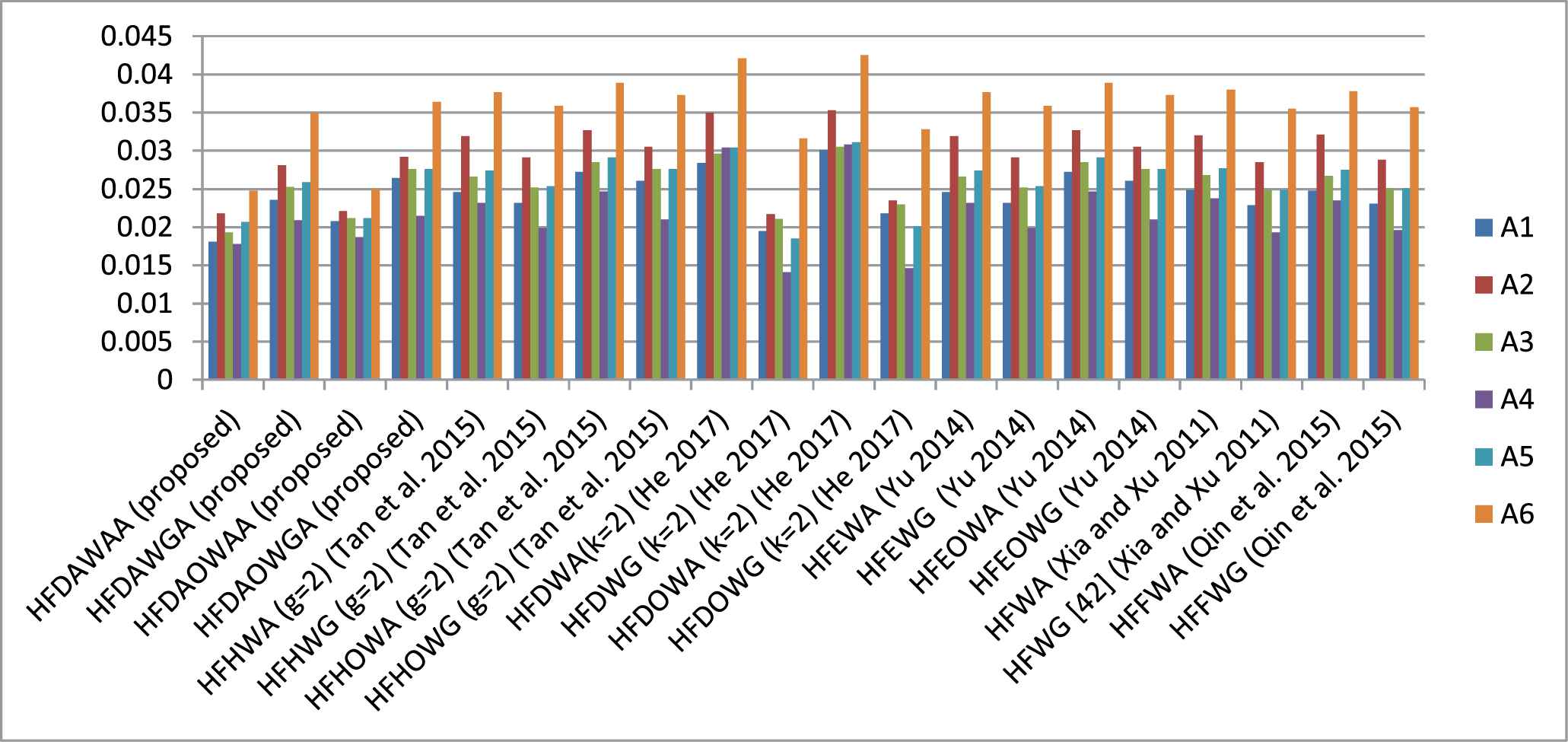
utilizing HFDAOWGA operator, the ranking orders are: A2≻A5=A3≻A1,A6≻A3≻A1≻A4, A6≻A2≻A5≻A4 and hence overall ranking order is: A6≻A2≻A5=A3≻A1≻A4 which validates the test criteria 2 and 3.

7. COMPARATIVE STUDY

In pursuance of performance comparison of the eloquent method developed by us discussed here with some existing MADM methods under hesitant fuzzy environment, we have conducted an analysis with some of the existing methods namely- Yu's method [55] using Hesitant fuzzy Einstein weighted arithmetic aggregation operator (HFEWA), Hesitant fuzzy Einstein weighted geometric aggregation operator (HFEWG), Hesitant fuzzy Einstein ordered weighted arithmetic aggregation operator (HFEOWA), and Hesitant fuzzy Einstein ordered weighted geometric aggregation operator (HFEOWG) operators [55]; Xia and Xu's method [43] using Hesitant fuzzy weighted arithmetic aggregation operator (HFWA) and Hesitant fuzzy weighted geometric aggregation operator (HFWG) operators; Qin et al.'s method [59] by using Hesitant fuzzy Frank weighted averaging operator (HFFWA) and Hesitant fuzzy Frank weighted geometric operator (HFFWG) operators; Tan et al.'s method [56] using Hesitant fuzzy Hamachar weighted arithmetic aggregation operator (HFHWA), Hesitant fuzzy Hamachar weighted geometric aggregation operator (HFHWG), Hesitant fuzzy Hamachar ordered weighted arithmetic aggregation operator (HFHOWA), and Hesitant fuzzy Hamachar ordered weighted geometric aggregation operator (HFHOWG) operators; and He's method [62] using Hesitant fuzzy Dombi weighted arithmetic aggregation operator (HFDWA), Hesitant fuzzy Dombi weighted geometric aggregation operator (HFDWG), Hesitant fuzzy Dombi ordered weighted arithmetic aggregation operator (HFDOWA), and Hesitant fuzzy Dombi ordered weighted geometric aggregation operator (HFDOWG) operators. We have utilized these operators in step-2 of the proposed algorithm. The final score values of the alternatives and the ranking order are summarized in a tabular form, numbered by 4. It is very much translucent from Table 4 that despite the appearance of slight difference occurs to the respective ranking order of the alternatives; the best i.e., most desirable alternative is absolutely same as found in the existing methods [43,55,56,59,62].

Operators	Score Values						Ranking Order
Operators	A₁	A₂	A₃	A₄	A₅	A₆	Ranking Order
HFDAWAA (proposed)	0.0181	0.0218	0.0193	0.0178	0.0207	0.0248	A6≻A2≻A5≻A3≻A1≻A4
HFDAWGA (proposed)	0.0236	0.0281	0.0253	0.0209	0.0259	0.0350	A6≻A2≻A5≻A3≻A1≻A4
HFDAOWAA (proposed)	0.0208	0.0221	0.0212	0.0187	0.0212	0.0250	A6≻A2≻A5=A3≻A1≻A4
HFDAOWGA (proposed)	0.0264	0.0292	0.0276	0.0215	0.0276	0.0364	A6≻A2≻A5=A3≻A1≻A4
HFHWA (γ = 2) [56]	0.0246	0.0319	0.0266	0.0232	0.0274	0.0377	A6≻A2≻A5≻A3≻A1≻A4
HFHWG (γ = 2) [56]	0.0232	0.0291	0.0252	0.0199	0.0254	0.0359	A6≻A2≻A5≻A3≻A1≻A4
HFHOWA (γ = 2) [56]	0.0272	0.0327	0.0285	0.0247	0.0291	0.0389	A6≻A2≻A5≻A3≻A1≻A4
HFHOWG (γ = 2) [56]	0.0261	0.0305	0.0276	0.0210	0.0276	0.0373	A6≻A2≻A5=A3≻A1≻A4
HFDWA (k = 2) [62]	0.0284	0.0350	0.0296	0.0304	0.0304	0.0421	A6≻A2≻A4≻A5≻A3≻A1
HFDWG (k = 2) [62]	0.0195	0.0217	0.0211	0.0141	0.0185	0.0316	A6≻A2≻A3≻A1≻A5≻A4
HFDOWA (k = 2) [62]	0.0301	0.0353	0.0305	0.0308	0.0311	0.0425	A6≻A2≻A5≻A4≻A3≻A1
HFDOWG (k = 2) [62]	0.0218	0.0235	0.0230	0.0146	0.0201	0.0328	A6≻A2≻A3≻A1≻A5≻A4
HFEWA [55]	0.0246	0.0319	0.0266	0.0232	0.0274	0.0377	A6≻A2≻A5≻A3≻A1≻A4
HFEWG [55]	0.0232	0.0291	0.0252	0.0199	0.0254	0.0359	A6≻A2≻A5≻A3≻A1≻A4
HFEOWA [55]	0.0272	0.0327	0.0285	0.0247	0.0291	0.0389	A6≻A2≻A5≻A3≻A1≻A4
HFEOWG [55]	0.0261	0.0305	0.0276	0.0210	0.0276	0.0373	A6≻A2≻A5≻A3≻A1≻A4
HFWA [43]	0.0249	0.0320	0.0268	0.0238	0.0277	0.0380	A6≻A2≻A5≻A3≻A1≻A4
HFWG [43]	0.0229	0.0285	0.0249	0.0193	0.0249	0.0355	A6≻A2≻A5=A3≻A1≻A4
HFFWA [59]	0.0248	0.0321	0.0267	0.0235	0.0275	0.0378	A6≻A2≻A5≻A3≻A1≻A4
HFFWG [59]	0.0231	0.0288	0.0251	0.0196	0.0251	0.0357	A6≻A2≻A5=A3≻A1≻A4

HFDAWAA, Hesitant fuzzy Dombi–Archimedean weighted arithmetic aggregation operator; HFDAWGA, Hesitant fuzzy Dombi–Archimedean weighted geometric aggregation operator; HFDAOWAA, Hesitant fuzzy Dombi–Archimedean ordered weighted arithmetic aggregation operator; HFDAOWGA, Hesitant fuzzy Dombi–Archimedean ordered weighted geometric aggregation operator; HFHWA, Hesitant fuzzy Hamachar weighted arithmetic aggregation operator; HFHWG, Hesitant fuzzy Hamachar weighted geometric aggregation operator; HFHOWA, Hesitant fuzzy Hamachar ordered weighted arithmetic aggregation operator; HFHOWG, Hesitant fuzzy Hamachar ordered weighted geometric aggregation operator; HFDWA, Hesitant fuzzy Dombi weighted arithmetic aggregation operator; HFDWG, Hesitant fuzzy Dombi weighted geometric aggregation operator; HFDOWA, Hesitant fuzzy Dombi ordered weighted arithmetic aggregation operator; HFDOWG, Hesitant fuzzy Dombi ordered weighted geometric aggregation operator; HFEWA, Hesitant fuzzy Einstein weighted arithmetic aggregation operator; HFEWG, Hesitant fuzzy Einstein weighted geometric aggregation operator; HFEOWA, Hesitant fuzzy Einstein ordered weighted arithmetic aggregation operator; HFEOWG, Hesitant fuzzy Einstein ordered weighted geometric aggregation operator; HFWA, Hesitant fuzzy weighted arithmetic aggregation operator; HFWG, Hesitant fuzzy weighted geometric aggregation operator; HFFWA, Hesitant fuzzy Frank weighted averaging operator; HFFWG, Hesitant fuzzy Frank weighted geometric operator.

Table 4

Comparative study with existing approaches.

Alongside the above comparative study (Table 4 and Figure 2), we discuss also some characteristic comparison of our proposed MADM approach and the decision-making methods suggested by Xia and Xu [43], Yu [55], Tan et al. [56], Qin et al. [59] and He [62], which are summarized in Table 5.

Methods	Whether Handle MADM Problems?	Whether Aggregation Operators Are in Generalized Form?	Whether the Aggregation Operators Are Flexible in Nature?	Whether the Method Reduces Computational Complexity?	Whether Compatible with Risk Preferences?
Xia and Xu [43]	Yes	No	No	Yes	No
Yu [55]	Yes	No	No	Yes	No
Tan et al. [56]	Yes	Yes	No	No	Yes
He [62]	Yes	No	No	Yes	Yes
Proposed	Yes	Yes	Yes	Yes	Yes

Table 5

Characteristic comparisons.

Thus, our proposed approach leads to the following advantageous facts:

The proposed AOs are obtained through the coalescence of the Dombi and Archimedean operations under HF environment and hence the raised MADM approach can be considered as one such blooming works because it develops a new flexible measure for decision-makers to choose the appropriate functions and parameters in accordance with the risk preferences whereas the existing methods [43,55,56,59,62] envisage the HF information in nonappearance of the simultaneous act of flexibility of functions and parameters.
Our proposed AOs include a parameter “k” which can try on the aggregate value based on the real decision needs. Thus, our proposed operators reveal themselves with higher generality and flexibility.

8. CONCLUSION

Keeping in mind the sensitive issue of growing perplexity and dubiousness of real-world decision-making problems, at the time of the formation of MADM, the attribute value is represented suitably as a HFE. The existing many information fusion methods developed so far for aggregating HF information, are restricted to algebraic t-norm and t-conorm, Einstein t-norm and t-conorm, Hammacher t-norm and t-conorm, and even we observe the inflexibility in the process of aggregation. Motivated by the idea of Dombi and Archimedean operations, in this paper, we have introduced some new operations between HFE. The prominent characteristics of these proposed operators are studied. Furthermore, we have developed some HF AOs based on the proposed operations, such as HFDAWAA, HFDAOWAA, HFDAHAA, HFDAWGA, HFDAOWGA, and HFDAHGA operators. Some essential properties such as idempotency, boundedness, shift invariance, monotonicity etc., of the proposed AOs are discussed in detail. Next, a procedure of MADM based on the proposed operators is presented under a HF environment. At the end, we fetch a practical example of a human resource selection to be comfortable with the decision steps in the proposed method. The result demonstrates the practicality and effectiveness of the new method.

CONFLICTS OF INTEREST

The authors declare that they don’t have any conflict of interest.

AUTHORS' CONTRIBUTIONS

Abhijit Saha: Conceptualization, methodology, validation, writing original draft; Peide Liu, Samarjit Kar, Debjit Dutta: Formal analysis, writing original draft, review and editing.

ACKNOWLEDGMENTS

This paper is supported by the National Natural Science Foundation of China (No. 71771140), Project of cultural masters and “the four kinds of a batch” talents, the Special Funds of Taishan Scholars Project of Shandong Province (No. ts201511045), Major bidding projects of National Social Science Fund of China (19ZDA080).

REFERENCES

1.S. Alonso, I.J. Pérez, F.J. Cabrerizo, and E. Herrera-Viedma, A linguistic consensus model for web 2.0 communities, Appl. Soft Comput., Vol. 13, 2013, pp. 149-157.

2.J. Wu, F. Chiclana, and E. Herrera-Viedma, Trust based consensus model for social network in an incomplete linguistic information context, Appl. Soft Comput., Vol. 35, 2015, pp. 827-839.

3.C.M. Cruz, C. Porcel, J. Bernabé-Moreno, and E. Herrera-Viedma, A model to represent users trust in recommender systems using ontologies and fuzzy linguistic modeling, Inf. Sci., Vol. 311, 2015, pp. 102-118.

4.I.J. Pérez, F.J. Cabrerizo, S. Alonso, and E. Herrera-Viedma, A new consensus model for group decision making problems with non-homogeneous experts, IEEE Trans. Syst. Man Cybern. Syst., Vol. 44, 2014, pp. 494-498.

5.C.T. Chen, Extensions of the TOPSIS for group decision-making under fuzzy environment, Fuzzy Sets Syst., Vol. 114, 2000, pp. 1-9.

6.T.Y. Chen, C.H. Chang, and J.F.R. Lu, The extended QUALIFLEX method for multiple criteria decision analysis based on interval type-2 fuzzy sets and applications to medical decision making, Eur. J. Oper. Res., Vol. 226, 2013, pp. 615-625.

7.A.H. Marbini and M. Tavana, An extension of the Electre I method for group decision-making under a fuzzy environment, Omega, Vol. 39, 2011, pp. 373-386.

8.S.P. Wan and D.F. Li, Fuzzy LINMAP approach to heterogeneous MADM considering comparisons of alternatives with hesitation degrees, Omega, Vol. 41, 2013, pp. 925-940.

9.M.S. Kuo, G.S. Liang, and W.C. Huang, Extensions of the multi-criteria analysis with pair-wise comparison under a fuzzy environment, Int. J. Approx. Reason., Vol. 43, 2006, pp. 268-285.

10.Y.C. Kuo and S.T. Lu, Using fuzzy multiple criteria decision making approach to enhance risk assessment for metropolitan construction projects, Int. J. Proj. Manag., Vol. 31, 2013, pp. 602-614.

11.E. Roghanian, J. Rahimi, and A. Ansari, Comparison of first aggregation and last aggregation in fuzzy group TOPSIS, Appl. Math. Modell., Vol. 34, 2010, pp. 3754-3766.

12.W. Wang, X. Liu, and Y. Qin, Multi-attribute group decision making models under interval type-2 fuzzy environment, Knowl. Based Syst., Vol. 30, 2012, pp. 121-128.

13.N. Chen, Z. Xu, and M. Xia, Correlation coefficients of hesitant fuzzy sets and their applications to clustering analysis, Appl. Math. Modell., Vol. 37, 2013, pp. 2197-2211.

14.V. Torra, Hesitant fuzzy sets, Int. J. Intell. Syst., Vol. 25, 2010, pp. 529-539.

15.V. Torra and Y. Narukawa, On hesitant fuzzy sets and decision, in 18th IEEE International Conference on Fuzzy Systems (Ueju Island, Korea), 2009, pp. 1378-1382.

16.Z. Xu and M. Xia, Distance and similarity measures for hesitant fuzzy sets, Inf. Sci., Vol. 18, 2011, pp. 2128-2138.

17.D.H. Peng, C.Y. Gao, and Z.F. Gao, Generalized hesitant fuzzy synergetic weighted distance measures and their application to multiple criteria decision-making, Appl. Math. Modell., Vol. 37, 2013, pp. 5837-5850.

18.B. Farhadinia, Information measures for hesitant fuzzy sets and interval-valued hesitant fuzzy sets, Inf. Sci., Vol. 240, 2013, pp. 129-144.

19.G. Qian, H. Wang, and X. Feng, Generalized hesitant fuzzy sets and their application in decision support system, Knowl. Based Syst., Vol. 37, 2013, pp. 357-365.

20.N. Chen, Z. Xu, and M. Xia, Interval-valued hesitant preference relations and their applications to group decision making, Knowl. Based. Syst., Vol. 37, 2013, pp. 528-540.

21.B. Zhu, Z. Xu, and M. Xia, Dual Hesitant Fuzzy Sets, J Appl Math., Vol. 2012, 2012, pp. 1-13.

22.R.M. Rodríguez, L. Martinez, and F. Herrera, Hesitant fuzzy linguistic term sets for decision making, IEEE Trans. Fuzzy Syst., Vol. 20, 2012, pp. 109-119.

23.N. Zhang and G. Wei, Extension of VIKOR method for decision making problem based on hesitant fuzzy set, Appl. Math. Modell., Vol. 37, 2013, pp. 4938-4947.

24.X. Zhang and Z. Xu, The TODIM analysis approach based on novel measured functions under hesitant fuzzy environment, Knowl. Based Syst., Vol. 61, 2014, pp. 48-58.

25.Y. Dong, X. Chen, and F. Herrera, Minimizing adjusted simple terms in the consensus reaching process with hesitant linguistic assessments in group decision making, Inf. Sci., Vol. 297, 2015, pp. 95-117.

26.B. Zhu and Z. Xu, Consistency measures for hesitant fuzzy linguistic preference relations, IEEE Trans. Fuzzy Syst., Vol. 22, 2014, pp. 35-45.

27.H. Wang and Z. Xu, Some consistency measures of extended hesitant fuzzy linguistic preference relations, Inf. Sci., Vol. 297, 2015, pp. 316-331.

28.N. Chen and Z. Xu, Hesitant fuzzy ELECTRE II approach: a new way to handle multi-criteria decision making problems, Inf. Sci., Vol. 292, 2015, pp. 175-197.

29.J.Q. Wang, J. Wang, Q.H. Chen, H.Y. Zhang, and X.H. Chen, An outranking approach for multi-criteria decision-making with hesitant fuzzy linguistic term sets, Inf. Sci., Vol. 280, 2014, pp. 338-351.

30.J. Wang, J.Q. Wang, H.Y. Zhang, and X.H. Chen, Multi-criteria decision-making based on hesitant fuzzy linguistic term sets: an outranking approach, Knowl. Based Syst., Vol. 86, 2015, pp. 224-236.

31.X. Zhang and Z. Xu, Interval programming method for hesitant fuzzy multi-attribute group decision making with incomplete preference over alternatives, Comput. Ind. Eng., Vol. 75, 2014, pp. 217-229.

32.J. Castro, M.J. Barranco, R.M. Rodriguez, and L. Martinez, Group recommendations based on hesitant fuzzy sets, Int. J. Intell. Syst., Vol. 33, 2018, pp. 2058-2077.

33.R.M. Rodríguez, A. Labella, G.D. Tre, and L. Martinez, A large scale consensus reaching process managing group hesitation, Knowl. Based Syst., Vol. 159, 2018, pp. 86-97.

34.H. Dinçer, S. Yüksel, and L. Martínez, Balanced score card-based analysis about European Energy Investment Policies: a hybrid hesitant fuzzy decision-making approach with quality function deployment, Expert Syst. Appl., Vol. 115, 2019, pp. 152-179.

35.B. Zhu, Z. Xu, and J. Xu, Deriving a ranking from hesitant fuzzy preference relations under group decision making, IEEE Trans. Cybern., Vol. 44, 2014, pp. 1328-1337.

36.X. Zhang and Z. Xu, Hesitant fuzzy agglomerative hierarchical clustering algorithms, Int. J. Syst. Sci., Vol. 46, 2015, pp. 562-576.

37.J. Ye, Correlation coefficient of dual hesitant fuzzy sets and its application to multiple attribute decision making, Appl. Math. Modell., Vol. 38, 2014, pp. 659-666.

38.H. Liao, Z. Xu, and X.J. Zeng, Novel correlation coefficients between hesitant fuzzy sets and their application in decision making, Knowl. Based Syst., Vol. 82, 2015, pp. 115-127.

39.H. Liu and R.M. Rodríguez, A fuzzy envelope for hesitant fuzzy linguistic term set and its application to multi-criteria decision making, Inf. Sci., Vol. 258, 2014, pp. 220-238.

40.N. Zhao, Z. Xu, and F. Liu, Uncertainty measures for hesitant fuzzy information, Int. J. Intell. Syst., Vol. 30, 2015, pp. 818-836.

41.R. Rodríguez, L. Martínez, V. Torra, Z. Xu, and F. Herrera, Hesitant fuzzy sets: state of the art and future directions, Int. J. Intell. Syst., Vol. 29, 2014, pp. 495-524.

42.Z. Xu, Hesitant Fuzzy Sets Theory, Springer, Cham, Switzerland, 2014.

43.M. Xia and Z. Xu, Hesitant fuzzy information aggregation in decision making, Int. J. Approx. Reason., Vol. 52, 2011, pp. 395-407.

44.M. Xia, Z. Xu, and N. Chen, Some hesitant fuzzy aggregation operators with their application in group decision making, Group Decis. Negotiat., Vol. 22, 2013, pp. 259-279.

45.G. Wei, Hesitant fuzzy prioritized operators and their application to multiple attribute decision making, Knowl. Based Syst., Vol. 31, 2012, pp. 176-182.

46.G. Wei, X. Zhao, and R. Lin, Some hesitant interval-valued fuzzy aggregation operators and their applications to multiple attribute decision making, Knowl. Based. Syst., Vol. 46, 2013, pp. 43-53.

47.G. Wei, X. Zhao, H. Wang, and R. Lin, Hesitant fuzzy Choquet integral aggregation operators and their applications to multiple attribute decision making, Int. Inf. Inst. Tokyo. Inf., Vol. 15, 2012, pp. 441-448.

48.B. Zhu, Z. Xu, and M. Xia, Hesitant fuzzy geometric Bonferroni means, Inf. Sci., Vol. 205, 2012, pp. 72-85.

49.Z. Zhang, Hesitant fuzzy power aggregation operators and their application to multiple attribute group decision making, Inf. Sci., Vol. 234, 2013, pp. 150-181.

50.Z. Zhang and C. Wu, Weighted hesitant fuzzy sets and their application to multi-criteria decision making, Br. J. Math. Comput. Sci., Vol. 4, 2014, pp. 1091-1123.

51.Z. Zhang, C. Wang, D. Tian, and K. Li, Induced generalized hesitant fuzzy operators and their application to multiple attribute group decision making, Comput. Ind. Eng., Vol. 67, 2014, pp. 116-138.

52.H. Liao and Z. Xu, Extended hesitant fuzzy hybrid weighted aggregation operators and their application in decision making, Soft Comput., Vol. 19, 2015, pp. 2551-2564.

53.W. Zhou and Z. Xu, Optimal discrete fitting aggregation approach with hesitant fuzzy information, Knowl. Based Syst., Vol. 78, 2015, pp. 22-33.

54.C. Wei, N. Zhao, and X. Tang, Operators and comparisons of hesitant fuzzy linguistic term sets, IEEE Trans. Fuzzy Syst., Vol. 22, 2014, pp. 575-585.

55.D. Yu, Some hesitant fuzzy information aggregation operators based on Einstein operational laws, Int. J. Intell. Syst., Vol. 29, 2014, pp. 320-340.

56.C. Tan, W. Yi, and X. Chen, Hesitant fuzzy Hamacher aggregation operators for multi-criteria decision making, Appl. Soft Comput., Vol. 26, 2015, pp. 325-349.

57.J. Qin, X. Liu, and W. Pedrycz, Hesitant fuzzy Maclaurin symmetric mean operators and its application to multiple-attribute decision making, Int. J. Fuzzy Syst., Vol. 17, 2015, pp. 509-520.

58.B. Zhu and Z. Xu, Hesitant fuzzy Bonferroni means for multi-criteria decision making, J. Oper. Res. Soc., Vol. 64, 2013, pp. 1831-1840.

59.J. Qin, X. Liu, and W. Pedrycz, Frank aggregation operators and their applications to hesitant fuzzy multiple attribute decision making, Appl. Soft Comput., Vol. 41, 2016, pp. 428-452.

60.H.C. Liao and Z. Xu, A VIKOR based method for hesitant fuzzy multi-criteria decision making, Fuzzy Optim. Decis. Mak., Vol. 12, 2016, pp. 372-392.

61.T. Mahmood, F. Mehmood, and Q. Khan, Cubic hesitant fuzzy sets and their applications to multi-criteria decision making, Int. J. Algeb. Stat., Vol. 5, 2016, pp. 19-51.

62.X. He, Typhoon disaster assessment based on Dombi hesitant fuzzy information aggregation operators, Nat. Haza., Vol. 90, 2018, pp. 1153-1175.

63.Z. Xu and W. Zhou, Consensus building with a group of decision makers under the hesitant probabilistic fuzzy environment, Fuzz. Optim. Decis. Mak., Vol. 16, 2017, pp. 481-503.

64.J.H. Park, Y.K. Park, and M.J. Son, Hesitant probabilistic fuzzy information aggregation using Einsteins operations, Inform., Vol. 9, 2018, pp. 1-28.

65.J.C.R. Alcantud and V. Torra, Decomposition theorems and extension principles for hesitant fuzzy sets, Inf. Fusion, Vol. 41, 2018, pp. 48-56.

66.R. Wang and Y. Li, Picture hesitant fuzzy set and its application to multi criteria decision making, Symmetry, Vol. 10, 2018, pp. 295.

67.Y. Wang, R. Zhang, and L. Quian, An improved A* algorithm based on hesitant fuzzy set theory for multi criteria acrtic route planning, Symmetry, Vol. 10, 2018, pp. 765.

68.H. Lioa, G. Si, Z. Xu, and H. Fujita, Hesitant fuzzy linguistic preference utility set and its application in selection of fire rescue plans, Int. J. Environ. Res. Publ. Health, Vol. 15, 2018, pp. 664.

69.N. Yalcin and N.Y. Pehlivan, Application of the fuzzy CODAS method based on fuzzy envelopes for hesitant fuzzy linguistic term sets: a case study on a personnel selection problem, Symmetry, Vol. 11, 2019, pp. 493.

70.J. Wu, X.D. Liu, Z.W. Wang, and S.T. Zhang, Dynamic emergency decision making method with probabilistic hesitant fuzzy information based on GM(1, 1) and TOPSIS, IEEE Access, Vol. 7, 2018, pp. 7054-7066.

71.J.C.R. Alcantud, G.S. Garcia, X. Peng, and J. Zhan, Dual extended hesitant fuzzy sets, Symmetry, Vol. 11, 2019, pp. 714.

72.X.D. Liu, Z.W. Wang, S.T. Zhang, and J.S. Liu, A novel approach to fuzzy cognitive map based on hesitant fuzzy sets for modeling risk impact on electric power system, Int. J. Comput. Intell. Syst., Vol. 12, 2019, pp. 842-854.

73.X. Liu, Z. Wang, S. Zhang, and J. Liu, Probabilistic hesitant fuzzy multiple attribute decision making based on regret theory for the evaluation of venture capital projects, Econom. Res., Vol. 33, 2020, pp. 672-697.

74.J. Dombi, A general class of fuzzy operators, the De Morgan class of fuzzy operators and fuzziness measures induced by fuzzy operators, Fuzzy Sets Syst., Vol. 8, 1982, pp. 149-163.

75.G. Klir and B. Yuan, Fuzzy Sets and Fuzzy Logic: Theory and Applications, Prentice Hall, Upper Saddle River, NJ, USA, 1995.

76.H.T. Nguyen and E.A. Walker, A First Course in Fuzzy Logic, CRC Press, Boca Raton, FL, USA, 1997.

77.E.P. Klement and R. Mesiar, Logical, Algebraic, Analytic and Probabilistic Aspects of Triangular Norms, Elsevier, New York, NY, USA, 2005.

78.F.E. Boran, S. Genc, and D. Akay, Personnel selection based on intuitionistic fuzzy sets, Hum. Factors Ergon. Manuf. Serv. Ind., Vol. 21, 2011, pp. 493-503.

79.X. Wang and E. Triantaphyllou, Ranking irregularities when evaluating alternatives by using some ELECTRE methods, Int. J. Manag. Sci., Vol. 36, 2008, pp. 45-63.

<Previous Article In Issue

Download article (PDF)

Next Article In Issue>

Journal: International Journal of Computational Intelligence Systems
Volume-Issue: 14 - 1
Pages: 386 - 411
Publication Date: 2020/12/22
ISSN (Online): 1875-6883
ISSN (Print): 1875-6891
DOI: 10.2991/ijcis.d.201215.003 How to use a DOI?
Open Access: This is an open access article distributed under the CC BY-NC 4.0 license (http://creativecommons.org/licenses/by-nc/4.0/).

Cite this article

ris enw bib

TY  - JOUR
AU  - Peide Liu
AU  - Abhijit Saha
AU  - Debjit Dutta
AU  - Samarjit Kar
PY  - 2020
DA  - 2020/12/22
TI  - Multi-Attribute Decision-Making Using Hesitant Fuzzy Dombi–Archimedean Weighted Aggregation Operators
JO  - International Journal of Computational Intelligence Systems
SP  - 386
EP  - 411
VL  - 14
IS  - 1
SN  - 1875-6883
UR  - https://doi.org/10.2991/ijcis.d.201215.003
DO  - 10.2991/ijcis.d.201215.003
ID  - Liu2020
ER  -

download .riscopy to clipboard