
Enhancing Whale Optimization Algorithm with Chaotic Theory for Permutation Flow Shop Scheduling Problem
 , Hui Hu3
- DOI
- 10.2991/ijcis.d.210112.002How to use a DOI?
- Keywords
- Whale optimization algorithm; Chaotic maps; Flow shop scheduling; Makespan; Local search; Cross selection
- Abstract
The permutation flow shop scheduling problem (PFSSP) is a typical production scheduling problem and it has been proved to be a nondeterministic polynomial (NP-hard) problem when its scale is larger than 3. The whale optimization algorithm (WOA) is a new swarm intelligence algorithm which performs well for PFSSP. But the stability is still low, and the optimization results are not too good. On this basis, we optimize the parameters of WOA through chaos theory, and put forward a chaotic whale algorithm (CWA). Firstly, in this paper, the proposed CWA is combined with Nawaz–Ensco–Ham (NEH) and largest-rank-value (LRV) rule to initialize the population. Next, chaos theory is applied to WOA algorithm to improve its convergence speed and stability. On this basis, we also use cross operator and reversal-insertion operator to enhance the search ability of the algorithm. Finally, the improved local search algorithm is used to optimize the job sequence to find the minimum makespan. In several experiments, different benchmarks are used to investigate the performance of CWA. The experimental results show that CWA has better performance than other scheduling algorithms.
- Copyright
- © 2021 The Authors. Published by Atlantis Press B.V.
- Open Access
- This is an open access article distributed under the CC BY-NC 4.0 license (http://creativecommons.org/licenses/by-nc/4.0/).
1. INTRODUCTION
The flow shop scheduling problem (FSSP) [1] is a job set allocation for a set of available machines in time to satisfy a set of performance indicators. Traditional FSSP includes a set of jobs, and each job is processed on all machines in a certain order. The goal of scheduling is to arrange jobs to each machine reasonably, and to arrange the processing order and start time of jobs reasonably, so that the constrained conditions can be used and some performance indicators can be optimized. Permutation flow shop scheduling problem (PFSSP) is an important problem in the actual production process, and it is one of the most difficult NP-hard problem [2]. In essence, it is a classical combinatorial optimization problem, involving n jobs and m machines. It is generally described that n jobs which needs to go through m processes need to be processed on m machines. Each process requires different machines, and n jobs have the same processing sequence on m machines which is different from FSSP. The traditional method is difficult to solve these problems, so the intelligent algorithms are required to solve these problems. Inspired by nature, these strong metaheuristic algorithms are applied to solve NP-hard problems such as scheduling [3–7], image [8–10], feature selection [11–13] and detection [14–16], path planning [17,18], cyber-physical social system [19,20], texture discrimination [21], factor evaluation [22], saliency detection [23], classification [24,25], object extraction [26], gesture segmentation [27], economic load dispatch [28,29], shape design [30], big data and large-scale optimization [31–33], signal processing [34], silencing efficacy prediction [35], multi-objective optimization [36,37], unit commitment [38,39], vehicle routing [40], knapsack problem [41–43] and fault diagnosis [44–46], and test-sheet composition [47].
Many methods are used to solve FSSP, such as ant colony optimization (ACO) [48,49], artificial bee colony (ABC) [50], genetic algorithms (GAs) [51,52], and some hybrid algorithms [53–57]. Among hybrid methods, how to schedule resources reasonably and efficiently is an important factor affecting the efficiency of the model, which has been widely concerned for a long time. Up to now, the study of swarm has been very widely. Furthermore, the method of biotechnology was explored and proved to be effective. The above algorithms are optimized iteratively to simulate the evolution of nature, so that the result approaches to the optimal solution. These algorithms are mainly realized by simulating the biological characteristics of nature, e.g., whale optimization algorithm (WOA) [58] simulates predation behavior of humpback whales, and it is used to solve PFSSP [59]. There are many methods to solve PFSSP before, but they have some problems such as slow convergence and easy to fall into local optimum. WOA is a new type of algorithm to solve this problem, and it is widely used in various fields, such as wind speed forecasting system [60], image segmentation [61], economic dispatch problem [62], and neural network [63], which imitates the behavior characteristics of animal neural network and carries out distributed parallel information processing. According to the different industrial environment, the heuristic algorithm mainly optimize the following two parameters in the quality of service (QoS):
Makespan—optimize the maximum makespan of the job scheduling so as to ensure the highest efficiency of the job processing.
Running time—the algorithm requires lower running time.
However, the stability of WOA is poor, and the experimental results also have a lot of room for optimization, so we proposed an algorithm—chaotic whale optimization algorithm (CWA) which achieves a better stability and a smaller makespan than WOA. This algorithm uses the WOA model and improves it on this basis. Firstly, in initialization stage, WOA is combined with Nawaz–Ensco–Ham (NEH) algorithm, and largest-rank-value (LRV) rule is used to transform continuous whale population into discrete job sequence. In this way, a more suitable initial population can be generated. Secondly, CWA adopts cross selection strategy, including cross operator and reversal-insertion operator, which makes the generated search agent better. Thirdly, we improve the local search strategy so that the algorithm can escape from local optimal solutions. Finally, and most importantly, we adopt the chaotic mapping strategy, which makes the generation of the next search agent affected by the last search agent. We incorporated the above strategies into WOA algorithm, and a new variant of WOA namely CWA was proposed for solving PFSSP problem. The experimental results indicated that CWA has better performance than WOA.
The remainder of the paper is organized as follows: Some methods reported in the literatures for FSSP are provided in Section 2. The PFSSP is represented in Section 3. The standard WOA is described in Section 4 and CWA algorithm is discussed in Section 5. The experimental results of CWA are shown in Section 6. This work ends in Section 7 with the conclusions and future work.
2. RELATED WORK
In this paper, we introduced chaos theory into WOA and proposed CWA method to solve PFSSP. Therefore, the latest literatures on PFSSP, search algorithms, and chaos theory are summarized and reviewed as follows.
2.1. Permutation Flow Shop Scheduling Problem
In the field of PFSSP, bio-inspired algorithms have achieved a lot of excellent results and PFSSP was proposed by Johnson in 1954 [64]. Over the next few years, there are also many mature algorithms that have been applied. Rossit et al. [65] reviewed the related work of PFSSP past decades and provided the future work orientation of PFSSP. Han et al. [66] proposed a bi-objective model consisting of robustness and stability, which improved the efficiency of flow shop scheduling and optimized the problem. At the same time, in order to reduce the makespan, Ruiz et al. [67] improved the initialization and processing of the algorithm, and enhanced the ability of local search. Liu et al. [68] proposed a different priority rule using skewness used in NEH [69] algorithm to reduce the makespan of PFSSP. Santucci et al. [70] made a special treatment of the search operator and changed the selection strategy, which made the algorithm reach an excellent level. ABC algorithm [71] is swarm intelligence algorithm that mimic natural creatures. Li et al. [72] studied bionic principles and applied ABC to solve PFSSP to reduce the makespan. Sioud and Gagné [73] chosen a suitable neighborhood and improved the migrating bird optimization algorithm by Tabu list and restart method. Finally, it is applied to PFSSP to complete the optimization of this problem. Pagnozzi and Stützle [74] redefined the framework of random local search algorithm (RLSA), and automatically matched the search algorithm to improve the performance of RLSA. In this way, the minimum makespan can be obtained efficiently. All the above algorithms have improved the flow shop scheduling, which provided a good reference for us to reduce makespan of PFSSP.
2.2. Search Algorithms
In terms of the implementation of search algorithm, there have been many fruitful research results. Wang and Tan [75] investigated a new idea of search algorithm, which is to reuse the previous individual search information. This method improved the quality of the subsequent population and had a good application in PFSSP. Benavides and Ritt [76] observed that the optimal scheduling usually includes a few local job inversion permutation structures, so they proposed an iterative local search algorithm. Gao et al. [77] proposed a new hybrid search algorithm, which introduced the balance strategy into the improved particle swarm optimization algorithm, and then combined with tabu search to achieve efficient search for FSSPs. Wang and Wang [78] improved the search algorithm according to the characteristics of other search algorithms. It included the improved initialization scheme based on NEH and other properties based on knowledge-based search algorithm. In addition, it also used critical path to improve the performance of the search algorithm. Kwong et al. [79] optimized the algorithm by changing the search direction of the search algorithm, and combined learning strategies to optimize the performance of the algorithm. In addition, we can combine different strategies to study new search algorithms. Fu et al. [80] combined different strategies such as explosive spark and selective solution, proposed a firework algorithm, and has a good optimization for flow shop scheduling.
Through the study on the search algorithms of flow shop scheduling, we proposed a strategy to change the search agent, and introduced a probability function to make the search results escape from the local optimal solution. These methods can achieve good results for PFSSP problems.
2.3. Chaos Theory
Chaos theory is the focus of this paper, and many achievements have been achieved in this field. Wang et al. [81] proposed a chaotic krill herd (KH) algorithm by studied the behavioral specialty of krill swarm and combined chaos theory. They used 12 chaotic mapping methods to improve the algorithm. Mokhtari and Noroozi [82] studied the chaotic map attraction characteristics in particle swarm optimization (PSO) and applied it to flow shop scheduling. Alatas [83] used chaotic mapping to improve the convergence of the algorithm and enabled ABC algorithm to escape from local optimal solution. At the same time, chaos theory can also be used in hybrid algorithm. Wang et al. [84] combines chaos theory with cuckoo algorithm to improve the performance of the algorithm.
In addition, chaos theory has a very important application in cryptography and image field, through which, the useful knowledge has been investigated. Xie et al. [85] combined cryptography with chaos and proposed a new encryption scheme, which is not inferior to the previous one. Abbasinezhad-Mood and Nikooghadam [86] used chaotic mapping to solve the key exchange problem in the process of cryptographic authentication. Chaotic mapping not only improved the security of the problem, but also made the method anonymous. Xu et al. [87] mainly proposed a bit-level image encryption algorithm based on chaotic mapping, which converted one image into two, and then replaced each other by chaotic control, thus it can complete image encryption. This encryption method has good encryption. The application of chaos theory is very extensive. We have applied the above ideas to PFSSP and achieved outstanding results.
Although there are many researches on flow shop scheduling, PFSSP still does not achieve the minimum makespan. By further improving the search algorithm and introducing chaos theory, the stability of the algorithm is greatly increased and the makespan is reduced.
3. PERMUTATION FLOW SHOP SCHEDULING PROBLEM
The mathematical description of the PFSSP with minimizing makespan is as follows.
The machine
PFSSP has the following requirements:
Each job
Each machine processes each job in the same processing sequence;
Each machine can only process one job at a time;
Each job can only be processed by one machine at a time;
The job must not be interrupted during the processing;
The buffer is infinite.
The processing sequence of jobs is
Therefore, the maximum completion time (makespan) can be defined as:
4. WOA AND CHAOTIC MAPS
4.1. Whale Optimization Algorithm
WOA [58] is a new swarm intelligence algorithm, which simulates the process of humpback whale predation, identifies prey, and circles around it. Algorithm 1 shows the implementation process of WOA. The WOA mainly consists of the three following processes: encircling prey, bubble-net attacking, and search for prey.
Algorithm 1: The standard WOA
Initialize a population of n random search agents
Evaluate all n search agents
w* = the best search agent
t = 0
While (t < iterations)
for each search agent
Update WOA parameters (a, A, C, l, and k)
if (k < 0.5)
if (|A| < l)
else if (|A| ≥ l)
end if
else if (k ≥ 0.5)
end if
end for
Evaluate the search agent
Update w* if
t = t + 1
end while
return w*
4.1.1. Encircling prey
Humpback whales swirl around prey in the course of predation and weave foam nets, and prey is gathered by bubbles. The voice makers of humpback whales make specific sounds at the bottom to push their prey to the surface. The best search location is determined by the location of the prey or the location close to the prey, and then updated according to the best search location. The strategy can be shown below:
4.1.2. Bubble-net attacking
Bubble-net attacking includes the following two behaviors: shrink ring of encirclement and continue to encircling prey. These two behaviors are modeled as the following equation:
4.1.3. Search for prey
The exploration of WOA can be achieved by random search agent xrand, which is different from exploitation using x*. This process can be given as follows:
4.2. Chaotic Maps
In this paper, the concept of chaotic optimization algorithm (COA) [88] is introduced, chaotic variables are used. Random variables make the results of functions randomly, while the use of chaotic variables avoids randomness, which makes the results more stable [81]. The nonrepetition and ergodicity of chaos makes the method using chaotic variables have faster convergence speed than the method using random variables [88]. In this paper, a one-dimensional irreversible chaotic mapping function is investigated. Table 1 lists twelve different chaotic maps [81].
| No. | Name | Definition |
|---|---|---|
| 1 | Chebyshev map | |
| 2 | Circle map* | |
| 3 | Gaussian map | |
| 4 | Intermittency map | |
| 5 | Iterative map | |
| 6 | Liebovitch map | |
| 7 | Logistic map | |
| 8 | Piecewise map | |
| 9 | Sine map | |
| 10 | Singer map | |
| 11 | Sinusoidal map | |
| 12 | Tent map |
Chaotic maps.
5. THE PROPOSED ALGORITHM
As a new intelligent algorithm, chaos optimization algorithm (COA) [81] has been widely studied and has been applied in many fields. In this paper, COA is firstly applied to the WOA of PFSSP, and a new algorithm called CWA is then proposed. CWA maps chaotic variables linearly to the value range of optimization variables, and optimizes the search process by using the randomness, ergodicity, and regularity of chaotic variables. For random variables, chaotic mapping changes the stability of variables and optimizes the convergence speed and performance of WOA. There are four processes that will be discussed below. The first three processes of CWA and WOA are similar, but CWA has more optimization of chaotic mapping process than WOA, so CWA has better performance than WOA. The time complexity of the four processes are O(N), O(N2), O(N), O(N), therefore, the time complexity of CWA is O(N2).
5.1. Initialization
For the initialization of PFSSP, firstly, we need to solve the problem of transforming continuous search agents into discrete job sequences. To solve this problem, we use the LRV rule [89] in CWA, which can effectively transform continuous values into discrete sequences. Secondly, we use the NEH algorithm [90] to initialize population. It includes the following steps:
These n jobs are arranged according to the decreasing order of machining time on the machine;
Take the first two jobs in the operation sequence and select the job sequence that minimized the makespan;
From the beginning of the third job, each job is inserted into each location sequence that already exists, and the sequence having smallest makespan is selected.
Afterwards, we need to calculate the maximum makespan of the generated sequence, i.e., to have a direct research of search agent performance, so as to get the best search agent. For example, we design a work sequence as shown in Table 2 and show the optimal scheduling sequence of this sequence, as shown in Table 3. Among them, the calculation of optimal scheduling sequence 1-4-3-2 is obtained by Eqs. (1–4). Some other sequences of this job scheduling are also shown in Table 4. The optimal job scheduling sequence is 1-4-3-2, corresponding to the completion time of this scheduling sequence, i.e., the optimal completion time, 64. Figure 1 shows the Gantt chart of the sequence 1-4-3-2.
| M1 | M2 | M3 | |
|---|---|---|---|
| J1 | 5 | 6 | 11 |
| J2 | 8 | 4 | 7 |
| J3 | 11 | 9 | 3 |
| J4 | 14 | 15 | 20 |
Job scheduling example.
| M1 | M2 | M3 | |
|---|---|---|---|
| J1 | 5 | 11 | 22 |
| J4 | 19 | 34 | 54 |
| J3 | 30 | 43 | 57 |
| J2 | 38 | 47 | 64 |
Evaluation of optimal scheduling sequence.
| Number | Job Sequence | Makespan |
|---|---|---|
| 1 | 2-3-4-1 | 79 |
| 2 | 4-1-3-2 | 70 |
| 3 | 3-1-2-4 | 73 |
| 4 | 4-3-2-1 | 70 |
| 5 | 1-4-3-2 | 64 |
Evaluation of different job scheduling,
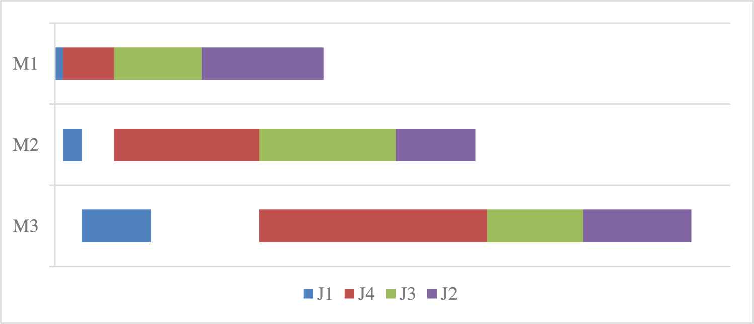
The Gantt chart for the job sequence 1-4-3-2.
5.2. Cross Selection
In this strategy, two operators are adopted in the experiment, namely cross operator and reversal-insertion operator.
5.2.1. Cross operator
This operator mainly exchanges the sequence of any two jobs and searches again. The main steps are as follows:
Two locations are randomly selected in the search agent, which are two jobs in the job sequence;
Exchange the order of these two jobs;
Evaluate makespan for new sequences.
The details of cross operator can be shown in Figure 2. The number of cross operators is related to the number of jobs. In this experiment, we set the number of cross operators as one percent of the number of jobs.

Cross operator.
5.2.2. Reversal-insertion operator
This operator is mainly to exchange the sequence of two adjacent jobs and insert them into other locations. The main steps are as follows:
Two adjacent locations are selected in the search agent, which are two adjacent jobs in the job sequence;
Swap the sequences of these two jobs and remove them from the current sequence which includes
Insert the exchanged jobs into the
Evaluate makespan for new sequences.
The details of cross operator can be shown in Figure 3.
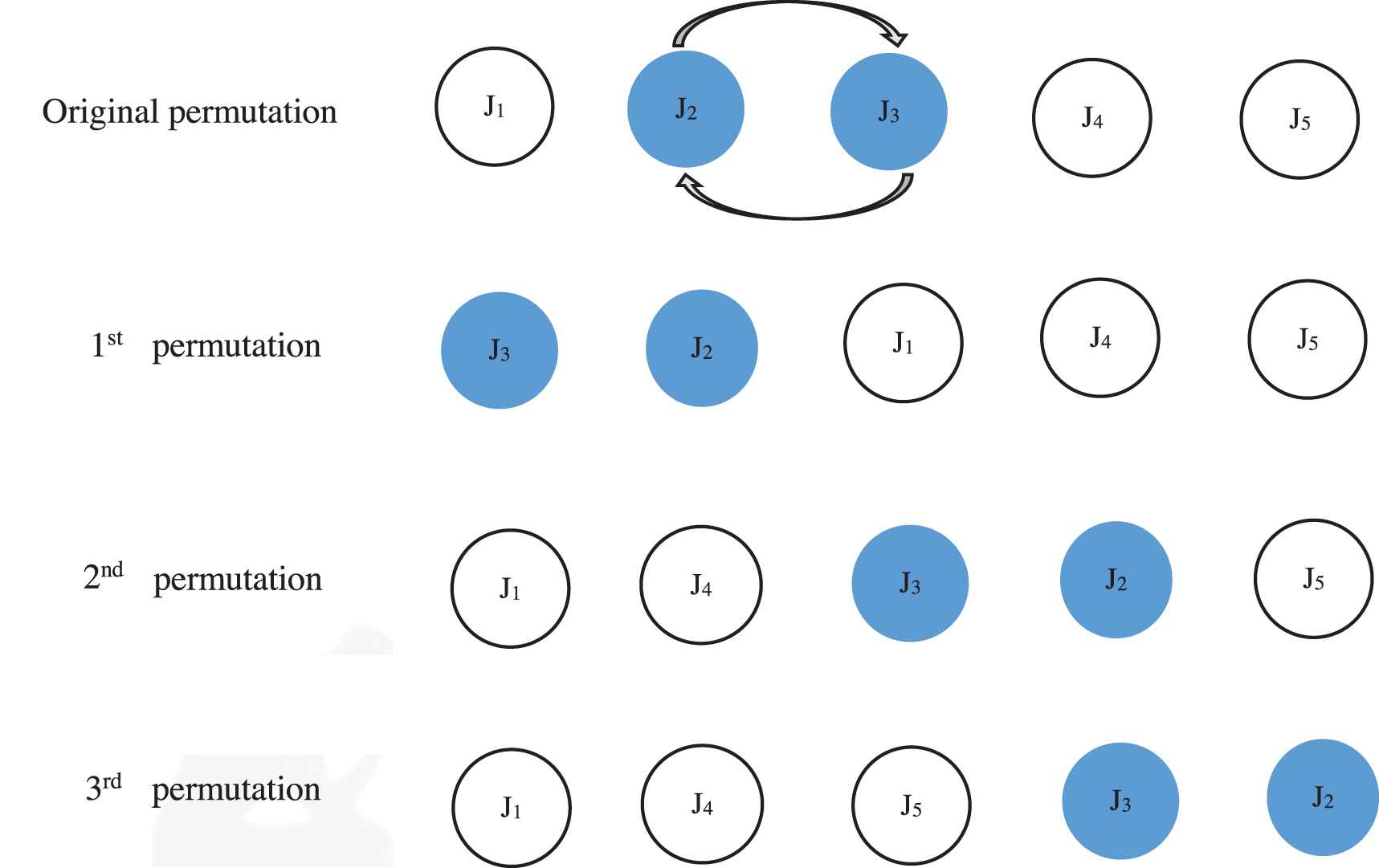
Reversal-insertion operator.
5.3. Local Search
The improved local search strategy is used to find better results than those obtained by WOA. For each job at generation t, move the job to each position in the sequence and find the minimum makespan. After the above strategies, an optimal search agent has been generated. The operator process can be provided as follows:
All search agents are orderly selected, and each selected search agent is removed from the job sequence which includes n jobs;
Insert the exchanged jobs into the
In order to avoid redundant computations, we make this strategy with small probability P.
5.4. Chaotic Mapping
According to Eqs. (11–13), the variable r affects the generation of search agents at the next iteration, which changes the performance and convergence of global search. Therefore, it is of great significance for the convergence of WOA and the generation of the next population.
Although the performance of standard WOA is satisfactory, there are still some deviations from the optimal results for PFSSP. In WOA, the variable r is randomly chosen between 0 and 1, which makes the next search agent more volatile. After introducing chaotic theory, we used chaotic mapping to change these parameters, which reduced the randomness of the algorithm and improved the performance and stability of the algorithm. Therefore, WOA using chaotic mapping is called chaotic WOA.
Algorithm 2 gives the basic process of CWA, and Figure 4 gives the basic framework of CWA.
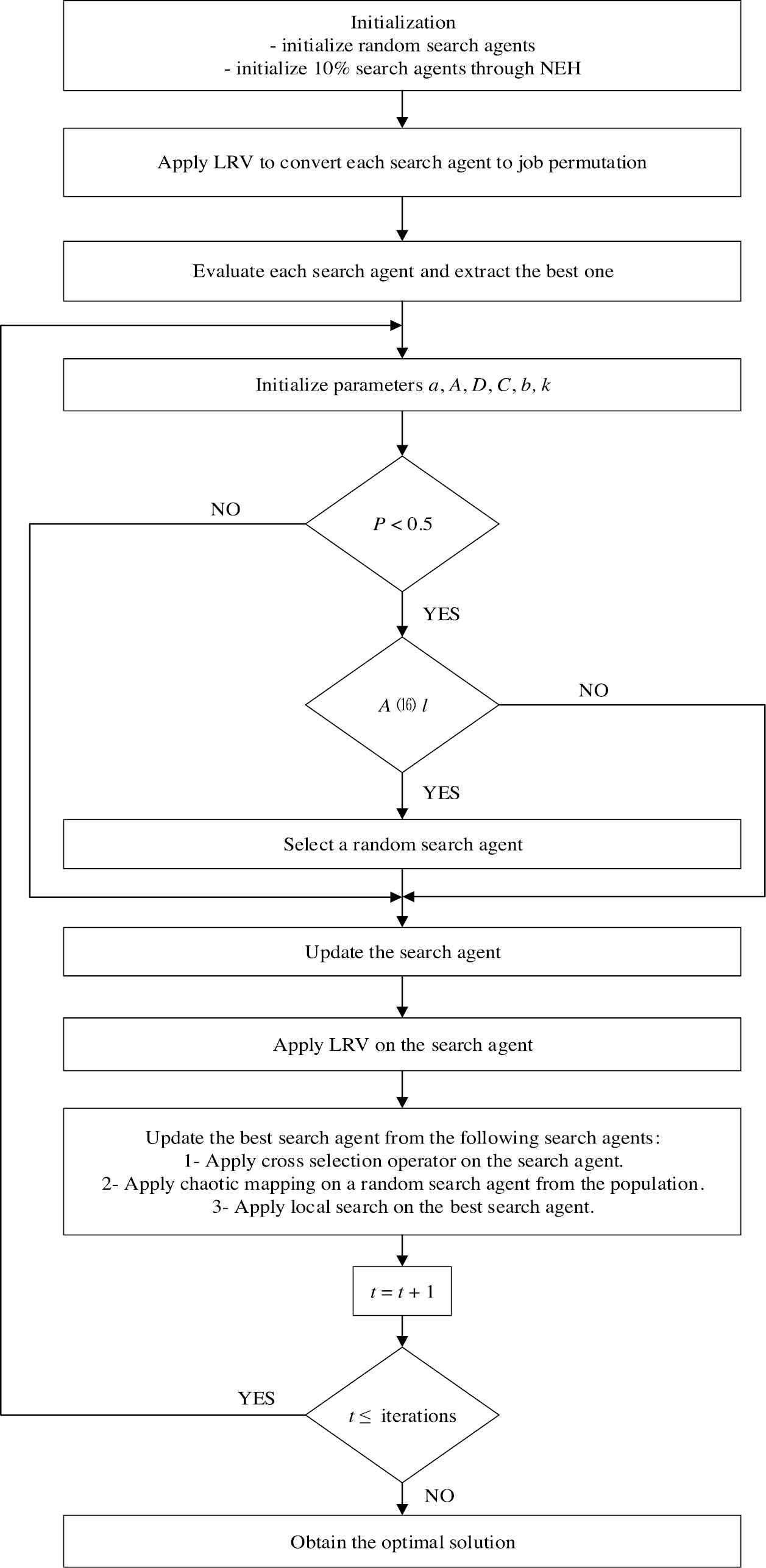
Framework of chaotic whale algorithm (CWA).
From Tables 5 and 6, we compare twelve different chaotic maps for WOA optimization through Reeves and Taillard benchmarks. M2 (Circle map) shows the best performance, so we get the Eq. (14), which is the best chaotic mapping of the variable r.
| No. | REC07 | REC13 | REC19 | REC27 | REC31 | REC39 |
|---|---|---|---|---|---|---|
| M1 | 1566.9 | 1964.2 | 2120.7 | 2418.4 | 3072.3 | 5170.3 |
| M2 | 1566.9 | 1938.8 | 2104.3 | 2396.8 | 3070.2 | 5167.0 |
| M3 | 1568.1 | 1966.1 | 2121.8 | 2416.2 | 3078.3 | 5177.2 |
| M4 | 1568.7 | 1966.5 | 2118.9 | 2417.6 | 3079.8 | 5170.1 |
| M5 | 1568.9 | 1950.6 | 2110.3 | 2402.0 | 3080.7 | 5167.8 |
| M6 | 1568.2 | 1956.7 | 2120.3 | 2416.6 | 3077.1 | 5173.6 |
| M7 | 1567.8 | 1966.9 | 2120.6 | 2417.0 | 3085.8 | 5169.9 |
| M8 | 1568.7 | 1965.3 | 2120.7 | 2398.7 | 3075.2 | 5170.1 |
| M9 | 1571.4 | 1961.0 | 2125.4 | 2414.7 | 3079.8 | 5168.2 |
| M10 | 1566.9 | 1962.3 | 2118.4 | 2416.8 | 3071.8 | 5168.6 |
| M11 | 1568.8 | 1969.7 | 2122.7 | 2411.4 | 3071.1 | 5169.0 |
| M12 | 1569.2 | 1940.4 | 2106.2 | 2410.8 | 3070.9 | 5183.7 |
The best experimental results are shown in bold.
The comparison of twelve chaotic maps on the Reeves benchmark.
| No. | Ta001 | Ta011 | Ta021 | Ta031 | Ta041 | Ta051 |
|---|---|---|---|---|---|---|
| M1 | 1281.8 | 1610.6 | 2346.4 | 2730.3 | 3054.3 | 3967.8 |
| M2 | 1278.2 | 1604.0 | 2346.0 | 2720.6 | 3043.6 | 3966.7 |
| M3 | 1279.9 | 1612.1 | 2355.9 | 2729.7 | 3045.8 | 3966.8 |
| M4 | 1278.2 | 1604.1 | 2348.2 | 2732.4 | 3051.0 | 3974.7 |
| M5 | 1278.2 | 1610.7 | 2356.6 | 2734.0 | 3045.8 | 3966.9 |
| M6 | 1281.8 | 1610.7 | 2359.9 | 2730.0 | 3046.0 | 3966.8 |
| M7 | 1279.9 | 1607.3 | 2354.8 | 2732.1 | 3047.9 | 3972.2 |
| M8 | 1279.9 | 1608.5 | 2355.3 | 2730.3 | 3046.8 | 3971.0 |
| M9 | 1281.9 | 1608.5 | 2354.8 | 2731.4 | 3043.6 | 3975.7 |
| M10 | 1280.9 | 1609.0 | 2348.5 | 2731.0 | 3047.1 | 3968.9 |
| M11 | 1279.9 | 1609.6 | 2349.5 | 2730.4 | 3049.1 | 3967.5 |
| M12 | 1279.9 | 1610.5 | 2353.5 | 2729.4 | 3049.8 | 3971.3 |
| No. | Ta061 | Ta071 | Ta081 | Ta091 | Ta101 | Ta111 |
| M1 | 5493.1 | 5804.0 | 6382.4 | 10939.0 | 11417.6 | 26572.2 |
| M2 | 5493.0 | 5798.4 | 6370.0 | 10914.0 | 11401.0 | 26550.1 |
| M3 | 5493.0 | 5826.0 | 6374.7 | 10927.9 | 11404.3 | 26554.3 |
| M4 | 5493.0 | 5809.1 | 6380.1 | 10931.2 | 11411.2 | 26557.0 |
| M5 | 5493.1 | 5799.3 | 6374.6 | 10927.2 | 11401.4 | 26540.2 |
| M6 | 5493.0 | 5803.0 | 6384.4 | 10933.0 | 11415.8 | 26566.3 |
| M7 | 5493.0 | 5801.8 | 6370.6 | 10934.2 | 11407.6 | 26557.4 |
| M8 | 5493.0 | 5800.6 | 6387.8 | 10921.1 | 11403.7 | 26551.7 |
| M9 | 5493.0 | 5800.3 | 6382.0 | 10938.6 | 11406.8 | 26554.2 |
| M10 | 5493.1 | 5801.2 | 6383.0 | 10922.6 | 11408.4 | 26572.7 |
| M11 | 5493.0 | 5799.6 | 6385.2 | 10927.9 | 11408.6 | 26550.1 |
| M12 | 5493.0 | 5803.0 | 6371.5 | 10926.2 | 11412.0 | 26576.5 |
The best experimental results are shown in bold.
The comparison of twelve chaotic maps on the Taillard benchmark.
6. EXPERIMENTAL RESULTS
In the field of flow shop scheduling, there are some well-known test functions studied in this paper to investigate the performance of CWA. Carlier consists of eight instances [91] and there is Reeves datasets [92] with twenty-one instances. In addition, there is only two instances, Heller data [93]. All of them can be found at http://people.brunel.ac.uk/~mastjjb/jeb/orlib/files/flowshop1.txt. The last one can be found at http://mistic.heig-vd.ch/taillard/problemes.dir/ordonnancement.dir/ordonnancement.html by Taillard [94] which has the largest number of instances (120). The proposed algorithm was written in Java and was run in the following conditions: Intel(R) Core(TM) i3-8100 CPU 3.60GHz which possesses 8G of RAM on Windows 10. The parameters of the proposed algorithm are presented in Table 7.
| Parameter | Value |
|---|---|
| Population size | 50 |
| Number of iterations | 3000 |
| Small probability P | 0.01 |
| Number of runs | 20 |
The parameters of the proposed algorithm.
6.1. The Comparison of WOA and CWA
Table 8 and Figure 5 show the standard deviation (STD) of WOA and CWA, which is defined as follows:
| Problem | WOA | CWA |
|---|---|---|
| REC07 | 9.44 | 0.92 |
| REC13 | 11.57 | 4.36 |
| REC19 | 11.43 | 2.91 |
| REC27 | 13.21 | 4.26 |
| REC31 | 15.56 | 3.36 |
| REC39 | 13.06 | 6.09 |
| Ta001 | 6.39 | 0.10 |
| Ta011 | 7.26 | 3.32 |
| Ta021 | 12.69 | 6.93 |
| Ta031 | 13.05 | 1.98 |
| Ta041 | 12.75 | 2.14 |
| Ta051 | 13.48 | 6.92 |
| Ta061 | 18.99 | 0.05 |
| Ta071 | 18.99 | 2.85 |
| Ta081 | 10.79 | 6.48 |
| Ta091 | 26.94 | 9.99 |
| Ta101 | 18.37 | 7.38 |
| Ta111 | 33.48 | 26.38 |
The standard deviation of WOA and CWA.
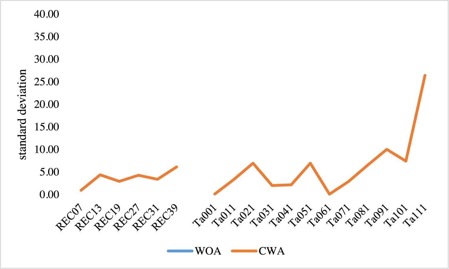
The standard deviation of whale optimization algorithm (WOA) and chaotic whale algorithm (CWA).
Table 8 shows the STD of the Reeves and Taillard benchmarks. The lower the numerical value, the higher the stability of the algorithm. In Figure 5, the numerical value of CWA is always lower than that of WOA, which proves that the addition of chaotic factor increases the stability of the algorithm.
6.2. The Comparison with Carlier, Reeves, and Heller Benchmarks
In this section, we compare the following algorithm with our CWA algorithm, as shown in Table 9. The comparative algorithms are as follows:
Hybrid genetic algorithm (HGA) [95]. HGA is a hybrid GA, which is used to solve the no wait FSSP with completion period as the goal.
Hybrid backtracking search algorithm (HBSA) [96]. Based on backtracking search algorithm (BSA), a HBSA is proposed for PFSP with the objective to minimize the makespan.
Discrete bat algorithm (DBA) [97]. DBA is constructed based on the idea of basic bat algorithm (BA), which divide whole scheduling problem into many subscheduling problems and then NEH heuristic be introduced to solve subscheduling problem.
Particle swarm optimization-based memetic algorithm (PSOMA) [98]. In the proposed PSOMA, both PSO-based searching operators and some special local searching operators are designed to balance the exploration and exploitation abilities. And the PSOMA utilizes several adaptive local searches to perform exploitation.
Particle swarm optimization based on variable neighborhood search (PSOVNS) [99]. A very efficient local search, called variable neighborhood search (VNS), was embedded in the PSO algorithm to solve the well-known benchmark suites in the literature.
| Problem | n * m | c* | HGA | HBSA | DBA | PSOMA | PSOVNS | CWA | |
|---|---|---|---|---|---|---|---|---|---|
| Car01 | 11*5 | 7038 | BRE | 0 | 0 | 0 | 0 | 0 | 0 |
| ARE | 0 | 0 | 0 | 0 | 0 | 0 | |||
| WRE | – | 0 | 0 | 0 | 0 | 0 | |||
| Car02 | 13*4 | 7166 | BRE | 0 | 0 | 0 | 0 | 0 | 0 |
| ARE | 0 | 0 | 0 | 0 | 0 | 0 | |||
| WRE | – | 0 | 0 | 0 | 0 | 0 | |||
| Car03 | 12*5 | 7312 | BRE | 0 | 0 | 0 | 0 | 0 | 0 |
| ARE | 0 | 0.06 | 0.397 | 0 | 0.42 | 0 | |||
| WRE | – | 1.19 | 1.109 | 0 | 1.189 | 0 | |||
| Car04 | 14*4 | 8003 | BRE | 0 | 0 | 0 | 0 | 0 | 0 |
| ARE | 0 | 0 | 0 | 0 | 0 | 0 | |||
| WRE | – | 0 | 0 | 0 | 0 | 0 | |||
| Car05 | 10*6 | 7720 | BRE | 0 | 0 | 0 | 0 | 0 | 0 |
| ARE | 0 | 0 | 0.018 | 0.018 | 0.039 | 0 | |||
| WRE | – | 0 | 0.375 | 0.375 | 0.389 | 0 | |||
| Car06 | 8*9 | 8505 | BRE | 0 | 0 | 0 | 0 | 0 | 0 |
| ARE | 0.04 | 0 | 0 | 0.076 | 0.076 | 0 | |||
| WRE | – | 0 | 0 | 0.764 | 0.764 | 0 | |||
| Car07 | 7*7 | 6590 | BRE | 0 | 0 | 0 | 0 | 0 | 0 |
| ARE | 0 | 0 | 0 | 0 | 0 | 0 | |||
| WRE | – | 0 | 0 | 0 | 0 | 0 | |||
| Car08 | 8*8 | 8366 | BRE | 0 | 0 | 0 | 0 | 0 | 0 |
| ARE | 0 | 0 | 0 | 0 | 0 | 0 | |||
| WRE | – | 0 | 0 | 0 | 0 | 0 | |||
| REC01 | 20*5 | 1247 | BRE | 0 | 0 | 0 | 0 | 0.16 | 0 |
| ARE | 0.14 | 0.14 | 0.08 | 0.144 | 0.168 | 0 | |||
| WRE | – | 0.16 | 0.16 | 0.16 | 0.321 | 0 | |||
| REC03 | 20*5 | 1109 | BRE | 0 | 0 | 0 | 0 | 0 | 0 |
| ARE | 0.09 | 0.08 | 0.081 | 0.189 | 0.158 | 0 | |||
| WRE | – | 0.18 | 0.18 | 0.721 | 0.18 | 0 | |||
| REC05 | 20*5 | 1242 | BRE | 0 | 0.24 | 0.242 | 0.242 | 0.242 | 0 |
| ARE | 0.29 | 0.24 | 0.242 | 0.249 | 0.249 | 0 | |||
| WRE | – | 0.24 | 0.242 | 0.402 | 0.42 | 0 | |||
| REC07 | 20*10 | 1566 | BRE | 0 | 0 | 0 | 0 | 0.702 | 0 |
| ARE | 0.69 | 0.46 | 0.575 | 0.986 | 1.095 | 0.169 | |||
| WRE | – | 1.15 | 1.149 | 1.149 | 1.405 | 0.83 | |||
| REC09 | 20*10 | 1537 | BRE | 0 | 0 | 0 | 0 | 0 | 0 |
| ARE | 0.64 | 0.07 | 0.638 | 0.621 | 0.651 | 0.046 | |||
| WRE | – | 0.65 | 2.407 | 1.691 | 1.366 | 0.325 | |||
| REC11 | 20*10 | 1431 | BRE | 0 | 0 | 0 | 0 | 0.071 | 0 |
| ARE | 1.1 | 0 | 1.167 | 0.129 | 1.153 | 0 | |||
| WRE | – | 0 | 2.655 | 0.978 | 2.656 | 0 | |||
| REC13 | 20*15 | 1930 | BRE | 0.36 | 0.1 | 0.415 | 0.259 | 1.036 | 0 |
| ARE | 1.68 | 0.53 | 1.461 | 0.893 | 1.79 | 0.458 | |||
| WRE | – | 1.14 | 3.782 | 1.502 | 2.643 | 0.829 | |||
| REC15 | 20*15 | 1950 | BRE | 0.56 | 0.05 | 0.154 | 0.051 | 0.769 | 0 |
| ARE | 1.12 | 0.64 | 1.226 | 0.628 | 1.487 | 0.574 | |||
| WRE | – | 1.18 | 2.103 | 1.076 | 2.256 | 1.026 | |||
| REC17 | 20*15 | 1902 | BRE | 0.95 | 0 | 0.368 | 0 | 0.999 | 0 |
| ARE | 2.32 | 1 | 1.277 | 1.33 | 2.453 | 0.672 | |||
| WRE | – | 2.16 | 2.154 | 2.155 | 3.365 | 1.419 | |||
| REC19 | 30*10 | 2093 | BRE | 0.62 | 0.29 | 0.573 | 0.43 | 1.529 | 0.287 |
| ARE | 1.32 | 0.81 | 0.929 | 1.313 | 2.099 | 0.538 | |||
| WRE | – | 1.29 | 2.023 | 2.102 | 2.532 | 1.051 | |||
| REC21 | 30*10 | 2017 | BRE | 1.44 | 0.69 | 1.438 | 1.437 | 1.487 | 0.642 |
| ARE | 1.57 | 1.5 | 1.671 | 1.596 | 1.671 | 1.472 | |||
| WRE | – | 1.83 | 2.231 | 1.636 | 2.033 | 1.636 | |||
| REC23 | 30*10 | 2011 | BRE | 0.4 | 0.45 | 0.796 | 0.596 | 1.343 | 0.348 |
| ARE | 0.87 | 1.28 | 1.173 | 1.31 | 2.106 | 0.85 | |||
| WRE | – | 3.08 | 2.381 | 2.038 | 2.884 | 1.939 | |||
| REC27 | 30*15 | 2373 | BRE | 1.1 | 0.25 | 1.011 | 1.348 | 1.728 | 0.011 |
| ARE | 1.83 | 1.27 | 1.419 | 1.605 | 2.463 | 1.004 | |||
| WRE | – | 2.57 | 2.298 | 2.402 | 3.203 | 1.728 | |||
| REC29 | 30*15 | 2287 | BRE | 1.4 | 0.57 | 1.049 | 1.442 | 1.968 | 0.499 |
| ARE | 2.7 | 1.42 | 2.58 | 1.888 | 3.109 | 1.243 | |||
| WRE | – | 2.97 | 3.935 | 2.492 | 4.067 | 2.317 | |||
| REC31 | 50*10 | 3045 | BRE | 0.43 | 0.43 | 2.299 | 1.51 | 2.594 | 0.427 |
| ARE | 1.34 | 1.91 | 3.392 | 2.254 | 3.232 | 0.99 | |||
| WRE | – | 2.66 | 4.532 | 2.692 | 4.237 | 1.478 | |||
| REC33 | 50*10 | 3114 | BRE | 0 | 0 | 0.61 | 0 | 0.835 | 0 |
| ARE | 0.78 | 0.59 | 0.728 | 0.645 | 1.007 | 0 | |||
| WRE | – | 1.28 | 1.734 | 0.834 | 1.477 | 0 | |||
| REC35 | 50*10 | 3277 | BRE | 0 | 0 | 0 | 0 | 0 | 0 |
| ARE | 0 | 0 | 0.037 | 0 | 0.038 | 0 | |||
| WRE | – | 0 | 0.092 | 0 | 0.092 | 0 | |||
| REC39 | 75*20 | 5087 | BRE | 2.2 | 0.9 | 2.28 | 1.553 | 2.85 | 0.081 |
| ARE | 2.79 | 1.88 | 3.851 | 2.426 | 3.371 | 1.573 | |||
| WRE | – | 3.38 | 5.347 | 2.83 | 3.951 | 1.985 | |||
| REC41 | 75*20 | 4960 | BRE | 3.64 | 1.69 | 3.81 | 2.641 | 4.173 | 1.457 |
| ARE | 4.92 | 2.72 | 5.095 | 3.684 | 4.867 | 2.347 | |||
| WRE | – | 3.55 | 6.532 | 4.052 | 5.585 | 3.044 |
Comparison on car and Rec benchmarks.
In Table 9, we use the best relative error (BRE), the average relative error (ARE), and the worst relative error (WRE) to measure the algorithm [59]. They are provided as follows:
Algorithm 2: The proposed CWA
Initialize a population of n random whales search agents
Apply LRV on each search to be mapped into job permutation
Solve the PFSSP using NEH
Choose about 10% random search agents from the population
and replace them with NEH
Evaluate all n search agents
w* = the best search agent
find w*
t = 0
While (t < iterations)
for each search agent
Update WOA parameters (a, A, C, l, and k)
if (k < 0.5)
if (|A| < l)
else if (|A| ≥ l)
end if
else if (k ≥ 0.5)
end if
end for
Apply LRV on each search agent
Perform cross selection strategy on the search agent
if
end if
Perform Chaotic mapping strategy on the search agent
if f(xr) < f(w*)
w* = xr
end if
w* = Perform local search strategy on the best search w*
Evaluate the search agent
Update w* if
t = t + 1
end while
return w*
Figures 6–8 shows the average value of BRE, ARE, and WRE on Table 9 about PSOVNS, PSOMA, DBA, HBSA, and CWA. The average values of CWA of BRE, ARE, and WRE are 0.14, 0.44, 0.73, respectively.
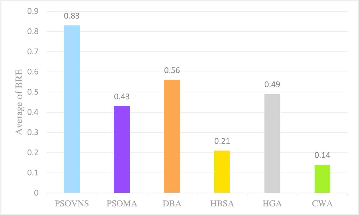
Average of best relative error (BRE).

Average of average relative error (ARE).
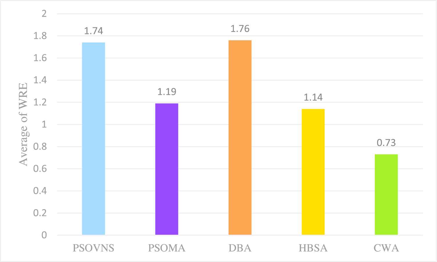
Average of worst relative error (WRE).
Table 9 shows the results of comparisons with other functions on Car and Rec benchmarks. The value in bold represents the best result. Looking at the Table 8, the scheduling results for each instance are different, but CWA's scheduling results are the best in both Car and Rec benchmarks.
Figure 6 reveals the average value of BRE. From Figure 6, CWA shows a shorter maximum completion time than the other five algorithms, and the scheduling results of HBSA are second only to CWA in terms of scheduling results.
Figure 7 displays the average of ARE. Compared with the best and worst values, the average value is the most suitable value to represent the performance of the algorithm. From Figure 7, for this case, CWA scheduling results are still better than other algorithms.
Figure 8 reveals the average value of WRE. It can be seen that even in the worst case, CWA is still the best method.
CWA is superior to the other five algorithms. It can be seen from the experimental results, CWA is very effective in the field of PFSSP.
Table 10 shows the experiments on Heller benchmark instances and compares them with NEH, SG [59], and DSOMA [100]. The CWA algorithm is not only superior to the three methods, but also better than the current known best values. Therefore, the 516 of Hel1 and 136 of Hel2 can be used as better-known results for later experimenters.
| Instance | n*m | Known Best | NEH | SG | DSOMA | CWA |
|---|---|---|---|---|---|---|
| Hel1 | 20*10 | 516 | 518 | 515 | 631 | 515 |
| Hel2 | 100*10 | 136 | 141 | 137 | 150 | 135 |
Comparison on Heller benchmark.
6.3. Comparison on Benchmark Taillard
In this section, we measure the performance of CWA on the Taillard benchmark instances and compare it with other algorithms. The best known value comes from [101]. This benchmark contains 120 examples, from the smallest 20*5 to the largest 500*20. We compare the Taillard function from the three aspects of the best scheduling, the average scheduling and the worst scheduling. In Table 11, we listed the experimental results of CWA and the following methods for best scheduling:
Discrete self-organizing migrating algorithm (DSOMA) [100]. New sampling routines have been developed that propagate the space between solutions in order to drive the algorithm.
Iterated greedy with referenced insertion scheme (IG_RIS) [102]. IG_RIS propose a constructive heuristic to generate an initial solution. In addition, an iteration jumping probability is proposed to change the neighborhood structure from insertion neighborhood to swap neighborhood.
Improved iterated greedy algorithm (IIGA) [103]. In the proposed IIGA, a speed-up method for the insert neighborhood is developed to evaluate the whole insert neighborhood of a single solution with
Hybrid genetic algorithm (HGA) [95]. HGA is a hybrid GA, which is used to solve the no wait FSSP with completion period as the goal.
Tabu-mechanism improved iterated greedy (TMIIG) [104]. The authors have modified the IG algorithm by utilizing a Tabu-based reconstruction strategy to enhance its exploration ability. A powerful neighborhood search method that involves insert, swap, and double-insert moves is then applied to obtain better solutions from the reconstructed solution in the previous step.
Discrete water wave optimization algorithm (DWWO) [105]. In refraction operator, a crossover strategy is employed by DWWO to avoid the algorithm falling into local optima.
| Instance | n*m | Known Best | DSOMA | IG_RIS | IIGA | HGA | TMIIG | DOOW | CWA |
|---|---|---|---|---|---|---|---|---|---|
| Ta001 | 20*5 | 1278 | 1374 | – | 1486 | 1449 | 1486 | 1486 | 1278 |
| Ta002 | 1359 | 1408 | – | 1528 | 1460 | 1528 | 1528 | 1359 | |
| Ta003 | 1081 | 1280 | – | 1460 | 1386 | 1460 | 1460 | 1081 | |
| Ta004 | 1293 | 1448 | – | 1588 | 1521 | 1588 | 1588 | 1293 | |
| Ta005 | 1235 | 1341 | – | 1449 | 1403 | 1449 | 1449 | 1235 | |
| Ta006 | 1195 | 1363 | – | 1481 | 1430 | 1481 | 1481 | 1195 | |
| Ta007 | 1239 | 1381 | – | 1483 | 1461 | 1483 | 1483 | 1239 | |
| Ta008 | 1206 | 1379 | – | 1482 | 1433 | 1482 | 1482 | 1206 | |
| Ta009 | 1230 | 1373 | – | 1469 | 1398 | 1469 | 1469 | 1230 | |
| Ta010 | 1108 | 1283 | – | 1377 | 1324 | 1377 | 1377 | 1108 | |
| Ta011 | 20*10 | 1582 | 1698 | – | 2044 | 1955 | 2044 | 2044 | 1586 |
| Ta012 | 1659 | 1833 | – | 2166 | 2123 | 2166 | 2166 | 1671 | |
| Ta013 | 1496 | 1676 | – | 1940 | 1912 | 1940 | 1940 | 1512 | |
| Ta014 | 1377 | 1546 | – | 1811 | 1782 | 1811 | 1811 | 1386 | |
| Ta015 | 1419 | 1617 | – | 1933 | 1933 | 1933 | 1933 | 1424 | |
| Ta016 | 1397 | 1590 | – | 1892 | 1827 | 1892 | 1892 | 1397 | |
| Ta017 | 1484 | 1622 | – | 1963 | 1944 | 1963 | 1963 | 1484 | |
| Ta018 | 1538 | 1731 | – | 2057 | 2006 | 2057 | 2057 | 1560 | |
| Ta019 | 1593 | 1747 | – | 1973 | 1908 | 1973 | 1973 | 1611 | |
| Ta020 | 1591 | 1782 | – | 2051 | 2001 | 2051 | 2051 | 1608 | |
| Ta021 | 20*20 | 2297 | 2436 | – | 2973 | 2912 | 2973 | 2973 | 2318 |
| Ta022 | 2099 | 2234 | – | 2852 | 2780 | 2852 | 2852 | 2122 | |
| Ta023 | 2326 | 2479 | – | 3013 | 2922 | 3013 | 3013 | 2345 | |
| Ta024 | 2223 | 2348 | – | 3001 | 2967 | 3001 | 3001 | 2237 | |
| Ta025 | 2291 | 2435 | – | 3003 | 2953 | 3003 | 3003 | 2296 | |
| Ta026 | 2226 | 2383 | – | 2998 | 2908 | 2998 | 2998 | 2235 | |
| Ta027 | 2273 | 2390 | – | 3052 | 2970 | 3052 | 3052 | 2293 | |
| Ta028 | 2200 | 2328 | – | 2839 | 2763 | 2839 | 2839 | 2216 | |
| Ta029 | 2237 | 2363 | – | 3009 | 2972 | 3009 | 3009 | 2245 | |
| Ta030 | 2178 | 2323 | – | 2979 | 2919 | 2979 | 2979 | 2195 | |
| Ta031 | 50*5 | 2724 | 3033 | 2974 | 3161 | 3127 | 3161 | 3170 | 2724 |
| Ta032 | 2834 | 3045 | 3171 | 3432 | 3438 | 3440 | 3441 | 2836 | |
| Ta033 | 2621 | 3036 | 2988 | 3211 | 3182 | 3213 | 3218 | 2622 | |
| Ta034 | 2751 | 3011 | 3113 | 3339 | 3289 | 3343 | 3349 | 2751 | |
| Ta035 | 2863 | 3128 | 3140 | 3356 | 3315 | 3361 | 3376 | 2863 | |
| Ta036 | 2829 | 3166 | 3158 | 3347 | 3324 | 3346 | 3352 | 2829 | |
| Ta037 | 2725 | 3021 | 3005 | 3231 | 3183 | 3234 | 3243 | 2725 | |
| Ta038 | 2683 | 3063 | 3040 | 3235 | 3243 | 3241 | 3239 | 2700 | |
| Ta039 | 2552 | 2908 | 2889 | 3072 | 3059 | 3075 | 3078 | 2554 | |
| Ta040 | 2782 | 3120 | 3094 | 3317 | 3301 | 3322 | 3330 | 2782 | |
| Ta041 | 50*10 | 2991 | 3638 | 3605 | 4274 | 4251 | 4274 | 4274 | 3025 |
| Ta042 | 2867 | 3511 | 3470 | 4177 | 4139 | 4179 | 4180 | 2905 | |
| Ta043 | 2839 | 3492 | 3465 | 4099 | 4083 | 4099 | 4099 | 2888 | |
| Ta044 | 3063 | 3672 | 3649 | 4399 | 4480 | 4399 | 4407 | 3063 | |
| Ta045 | 2976 | 3633 | 3614 | 4322 | 4316 | 4324 | 4324 | 3006 | |
| Ta046 | 3006 | 3621 | 3574 | 4289 | 4282 | 4290 | 4294 | 3020 | |
| Ta047 | 3093 | 3704 | 3667 | 4420 | 4376 | 4420 | 4420 | 3115 | |
| Ta048 | 3037 | 3572 | 3549 | 4318 | 4304 | 4321 | 4323 | 3042 | |
| Ta049 | 2897 | 3541 | 3510 | 4155 | 4162 | 4158 | 4155 | 2904 | |
| Ta050 | 3065 | 3624 | 3603 | 4283 | 4232 | 4286 | 4286 | 3099 | |
| Ta051 | 50*20 | 3850 | 4511 | 4484 | 6129 | 6138 | 6129 | 6129 | 3934 |
| Ta052 | 3704 | 4288 | 4262 | 5725 | 5721 | 5725 | 5725 | 3797 | |
| Ta053 | 3640 | 4289 | 4261 | 5862 | 5847 | 5873 | 5862 | 3717 | |
| Ta054 | 3720 | 4378 | 4338 | 5788 | 5781 | 5789 | 5789 | 3790 | |
| Ta055 | 3610 | 4271 | 4249 | 5886 | 5891 | 5886 | 5886 | 3715 | |
| Ta056 | 3681 | 4202 | 4271 | 5863 | 5875 | 5874 | 5871 | 3785 | |
| Ta057 | 3704 | 4315 | 4291 | 5962 | 5937 | 5968 | 5969 | 3781 | |
| Ta058 | 3691 | 4326 | 4298 | 5926 | 5919 | 5940 | 5926 | 3797 | |
| Ta059 | 3743 | 4329 | 4304 | 5876 | 5839 | 5876 | 5876 | 3852 | |
| Ta060 | 3756 | 4422 | 4398 | 5958 | 5935 | 5959 | 5958 | 3812 | |
| Ta061 | 100*5 | 5493 | 6151 | 6038 | 6397 | 6492 | 6397 | 6433 | 5493 |
| Ta062 | 5268 | 6064 | 5933 | 6234 | 6353 | 6246 | 6268 | 5268 | |
| Ta063 | 5175 | 6003 | 5837 | 6121 | 6148 | 6133 | 6162 | 5175 | |
| Ta064 | 5014 | 5786 | 5661 | 6026 | 6080 | 6028 | 6055 | 5023 | |
| Ta065 | 5250 | 6021 | 5873 | 6200 | 6254 | 6206 | 6221 | 5250 | |
| Ta066 | 5135 | 5869 | 5732 | 6074 | 6177 | 6088 | 6121 | 5135 | |
| Ta067 | 5246 | 6004 | 5890 | 6247 | 6257 | 6254 | 6311 | 5247 | |
| Ta068 | 5094 | 5924 | 5785 | 6130 | 6225 | 6150 | 6197 | 5099 | |
| Ta069 | 5448 | 6154 | 6029 | 6370 | 6443 | 6391 | 6418 | 5453 | |
| Ta070 | 5322 | 6186 | 6049 | 6381 | 6441 | 6396 | 6404 | 5328 | |
| Ta071 | 100*10 | 5770 | 7042 | 6896 | 8077 | 8115 | 8080 | 8093 | 5785 |
| Ta072 | 5349 | 6813 | 6622 | 7880 | 7986 | 7888 | 7891 | 5391 | |
| Ta073 | 5676 | 6943 | 6766 | 8028 | 8057 | 8042 | 8047 | 5691 | |
| Ta074 | 5781 | 7198 | 7037 | 8348 | 8327 | 8350 | 8364 | 5830 | |
| Ta075 | 5467 | 6815 | 6690 | 7958 | 7991 | 7967 | 7966 | 5497 | |
| Ta076 | 5303 | 6685 | 6517 | 7801 | 7823 | 7808 | 7791 | 5308 | |
| Ta077 | 5595 | 6827 | 6684 | 7866 | 7915 | 7880 | 7881 | 5638 | |
| Ta078 | 5617 | 6874 | 6729 | 7913 | 7939 | 7912 | 7924 | 5660 | |
| Ta079 | 5871 | 6092 | 6908 | 8161 | 8226 | 8164 | 8152 | 5840 | |
| Ta080 | 5845 | 6990 | 6832 | 8114 | 8186 | 8130 | 8126 | 5860 | |
| Ta081 | 100*20 | 6202 | 7854 | 7683 | 10700 | 10745 | 10722 | 10727 | 6357 |
| Ta082 | 6183 | 7910 | 7739 | 10594 | 10655 | 10611 | 10604 | 6314 | |
| Ta083 | 6271 | 7825 | 7697 | 10611 | 10672 | 10629 | 10624 | 6356 | |
| Ta084 | 6269 | 7902 | 7730 | 10607 | 10630 | 10615 | 10615 | 6359 | |
| Ta085 | 6314 | 7901 | 7694 | 10539 | 10548 | 10563 | 10551 | 6421 | |
| Ta086 | 6364 | 7921 | 7745 | 10690 | 10700 | 10684 | 10680 | 6468 | |
| Ta087 | 6268 | 8051 | 7848 | 10825 | 10827 | 10832 | 10824 | 6406 | |
| Ta088 | 6401 | 8025 | 7879 | 10839 | 10863 | 10846 | 10839 | 6548 | |
| Ta089 | 6275 | 7969 | 7771 | 10723 | 10751 | 10763 | 10745 | 6393 | |
| Ta090 | 6434 | 8036 | 7818 | 10798 | 10794 | 10797 | 10787 | 6538 | |
| Ta091 | 200*10 | 10862 | 13507 | 13100 | 15319 | 15739 | 15377 | 15418 | 10885 |
| Ta092 | 10480 | 13458 | 13048 | 15085 | 15534 | 15167 | 15252 | 10551 | |
| Ta093 | 10922 | 13521 | 13135 | 15376 | 15755 | 15416 | 15412 | 10948 | |
| Ta094 | 10889 | 13686 | 13112 | 15200 | 15842 | 15250 | 15304 | 10893 | |
| Ta095 | 10524 | 13547 | 13097 | 15209 | 15692 | 15268 | 15277 | 10537 | |
| Ta096 | 10326 | 13247 | 12869 | 15109 | 15622 | 15163 | 15222 | 10375 | |
| Ta097 | 10854 | 13910 | 13351 | 15395 | 15877 | 15441 | 15459 | 10868 | |
| Ta098 | 10730 | 13830 | 13225 | 15237 | 15733 | 15295 | 15307 | 10792 | |
| Ta099 | 10438 | 13410 | 13036 | 15100 | 15573 | 15155 | 15186 | 10465 | |
| Ta100 | 10675 | 13744 | 13119 | 15340 | 15803 | 15382 | 15378 | 10690 | |
| Ta101 | 200*20 | 11195 | 15027 | 14484 | 19681 | 20148 | 19723 | 19724 | 11355 |
| Ta102 | 11203 | 15211 | 14690 | 20096 | 20539 | 20127 | 20091 | 11438 | |
| Ta103 | 11281 | 15247 | 14776 | 19913 | 20511 | 19973 | 19989 | 11517 | |
| Ta104 | 11275 | 15174 | 14694 | 19928 | 20461 | 19997 | 19940 | 11504 | |
| Ta105 | 11259 | 15047 | 14547 | 19843 | 20339 | 19900 | 19875 | 11397 | |
| Ta106 | 11176 | 15212 | 14734 | 19942 | 20501 | 20003 | 19980 | 11366 | |
| Ta107 | 11360 | 15168 | 14744 | 20112 | 20680 | 20145 | 20119 | 11544 | |
| Ta108 | 11334 | 15247 | 14763 | 20056 | 20614 | 20053 | 20053 | 11537 | |
| Ta109 | 11192 | 15136 | 14643 | 19918 | 20300 | 19998 | 19932 | 11406 | |
| Ta110 | 11288 | 15243 | 14703 | 19935 | 20437 | 19932 | 19916 | 11551 | |
| Ta111 | 500*20 | 26059 | 37064 | 35372 | 46689 | 49095 | 47046 | 46871 | 26483 |
| Ta112 | 26520 | 37419 | 35743 | 47275 | 49461 | 47630 | 47294 | 26890 | |
| Ta113 | 26371 | 37059 | 35452 | 46544 | 48777 | 46977 | 46846 | 26717 | |
| Ta114 | 26456 | 37014 | 35687 | 46899 | 49283 | 47328 | 47185 | 26768 | |
| Ta115 | 26334 | 36894 | 35417 | 46741 | 48950 | 47238 | 47037 | 26611 | |
| Ta116 | 26477 | 37372 | 35747 | 46941 | 49533 | 47553 | 47166 | 26767 | |
| Ta117 | 26389 | 36998 | 35395 | 46509 | 48943 | 46944 | 46794 | 26639 | |
| Ta118 | 26560 | 36944 | 35568 | 46873 | 49277 | 47346 | 47127 | 26873 | |
| Ta119 | 26005 | 36862 | 35304 | 46743 | 49207 | 47205 | 47025 | 26282 | |
| Ta120 | 26457 | 37098 | 35643 | 46847 | 49092 | 47374 | 47105 | 26735 |
Comparison on Taillard benchmark based on the best scheduling.
The bold in Table 11 represents the best value of each instance. It is obvious that the best value of each instance is obtained by CWA, so the performance of CWA is better than the other six algorithms.
Table 11 shows the results of comparisons with other six methods on Taillard benchmark based on the best scheduling and this table gives the value of scheduling time directly. Because the scale of Taillard benchmark is relatively large, so we can see that when the size of the instance is relatively small, CWA can achieve the optimal scheduling, but with the increment of the size of the instance, it is difficult to achieve the optimal scheduling. Even if the optimal scheduling value is not reached, it is close to this value, and among the seven algorithms, the maximum completion time of CWA is the smallest.
Figure 9 shows the average error (AE) [59] of best scheduling, which is defined as follows:
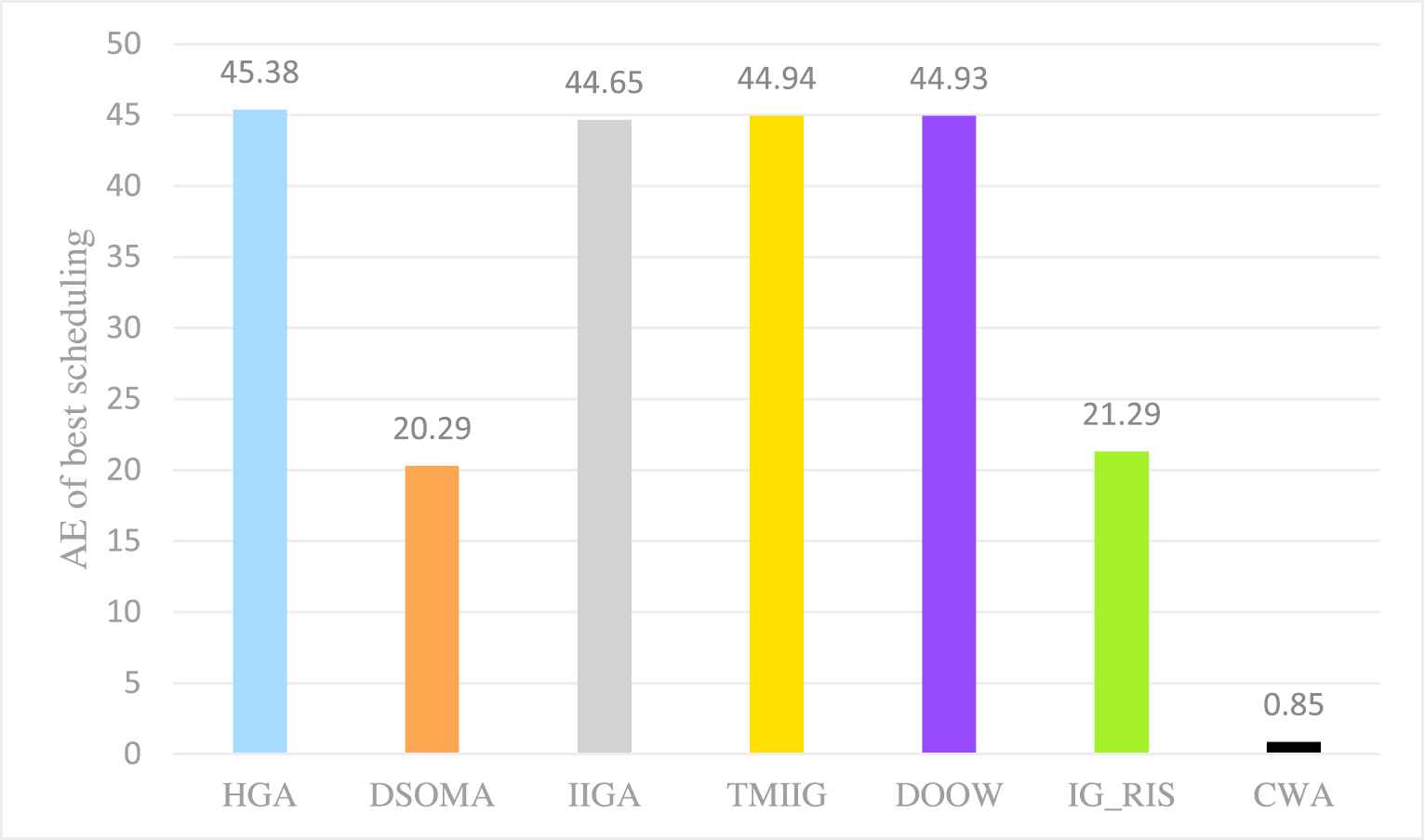
Average error (AE) of best scheduling.
From Figure 9, the performance of DSOMA is second only to CWA, but the AE of DSOMA is 24 times that of CWA. The performance of CWA is much better than other algorithms.
Figure 10 shows the degree of improvement of CWA of best scheduling relative to other algorithms, called improvement percentage (IP) [59], which is defined as follows:
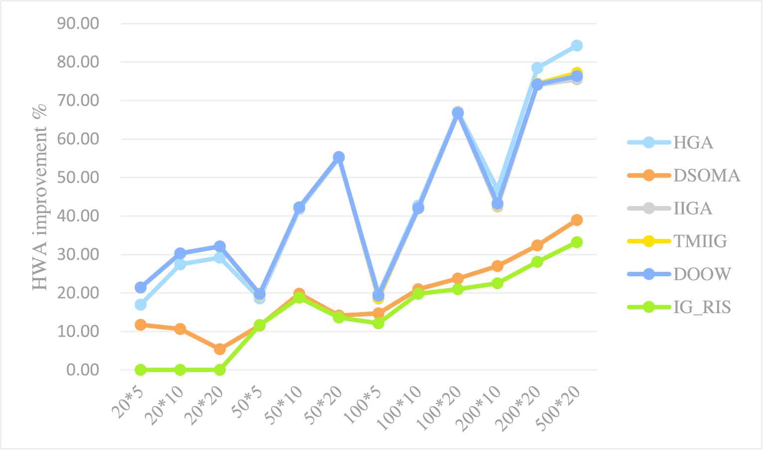
Improvement percentage (IP) of chaotic whale algorithm (CWA) based on the best scheduling.
In Figure 10, the IP of HGA, DOOW, TMIIG, and IIGA are comparatively similar, which indicates that their performance on Taillard benchmark is comparatively close. What's more, CWA outperforms HGA and DOOW to the greatest extent and IG_RIS to the smallest extent, but it outperforms all these algorithms.
Table 12 compares the average scheduling time of the Taillard benchmark, as compared with the following algorithm:
Nawaz-Enscore-Ham (NEH) [90]
Tabu-mechanism improved iterated greedy (TMIIG) [104]
Improved iterated greedy algorithm (IIGA) [103]
Hybrid genetic algorithm (HGA) [95]
Discrete water wave optimization algorithm (DWWO) [105]
| Instance | n*m | Known Best | NEH | TMIIG | IIGA | HGA | DWWO | CWA |
|---|---|---|---|---|---|---|---|---|
| Ta001 | 20*5 | 1278 | 1299 | 1486 | 1486 | 1472.7 | 1486 | 1278 |
| Ta002 | 1359 | 1365 | 1528 | 1528 | 1477.6 | 1528 | 1359 | |
| Ta003 | 1081 | 1132 | 1460 | 1460 | 1406.8 | 1460 | 1081 | |
| Ta004 | 1293 | 1329 | 1588 | 1588 | 1546.4 | 1588 | 1293 | |
| Ta005 | 1235 | 1305 | 1449 | 1449 | 1426.6 | 1449 | 1235 | |
| Ta006 | 1195 | 1251 | 1481 | 1481 | 1446.6 | 1481 | 1195 | |
| Ta007 | 1239 | 1251 | 1483 | 1483 | 1479.4 | 1483 | 1239 | |
| Ta008 | 1206 | 1215 | 1482 | 1482 | 1459.2 | 1482 | 1206 | |
| Ta009 | 1230 | 1284 | 1469 | 1469 | 1409.2 | 1469 | 1230 | |
| Ta010 | 1108 | 1127 | 1377 | 1377 | 1345.5 | 1377 | 1108 | |
| Ta011 | 20*10 | 1582 | 1681 | 2044 | 2044 | 1972.6 | 2044 | 1604 |
| Ta012 | 1659 | 1766 | 2166 | 2166 | 2154.6 | 2166 | 1691 | |
| Ta013 | 1496 | 1562 | 1940.4 | 1940 | 1931.1 | 1940 | 1530.5 | |
| Ta014 | 1377 | 1416 | 1811 | 1811 | 1794.3 | 1811 | 1409.35 | |
| Ta015 | 1419 | 1502 | 1933 | 1933 | 1934.4 | 1933 | 1450.75 | |
| Ta016 | 1397 | 1456 | 1892 | 1892 | 1850 | 1892 | 1423.05 | |
| Ta017 | 1484 | 1531 | 1963 | 1963 | 1951.5 | 1963 | 1500.35 | |
| Ta018 | 1538 | 1626 | 2057 | 2058.6 | 2038.5 | 2057 | 1577.4 | |
| Ta019 | 1593 | 1639 | 1973 | 1973 | 1953.9 | 1973 | 1620.5 | |
| Ta020 | 1591 | 1656 | 2051 | 2051 | 2019.3 | 2051 | 1633.05 | |
| Ta021 | 20*20 | 2297 | 2443 | 2973 | 2973 | 2938.5 | 2973 | 2346 |
| Ta022 | 2099 | 2134 | 2852 | 2852 | 2814.2 | 2852 | 2146.9 | |
| Ta023 | 2326 | 2414 | 3019.4 | 3019.4 | 2962.4 | 3014.3 | 2381.15 | |
| Ta024 | 2223 | 2257 | 3001 | 3001 | 2982.5 | 3001 | 2273.5 | |
| Ta025 | 2291 | 2370 | 3003 | 3003 | 2995.1 | 3003 | 2340.6 | |
| Ta026 | 2226 | 2349 | 2998 | 2998 | 2932.8 | 2998 | 2243.9 | |
| Ta027 | 2273 | 2383 | 3052 | 3052 | 3004.8 | 3052 | 2316.75 | |
| Ta028 | 2200 | 2249 | 2839 | 2839 | 2789.5 | 2839 | 2242.05 | |
| Ta029 | 2237 | 2306 | 3009 | 3009 | 3005.3 | 3009 | 2282.55 | |
| Ta030 | 2178 | 2257 | 2979 | 2979 | 2956.3 | 2979 | 2242.9 | |
| Ta031 | 50*5 | 2724 | 2729 | 3162.4 | 3222 | 3198.3 | 3171.8 | 2720.6 |
| Ta032 | 2834 | 2882 | 3441 | 3474.4 | 3453.1 | 3444.5 | 2837.9 | |
| Ta033 | 2621 | 2650 | 3216 | 3262.8 | 3242.5 | 3231.8 | 2624.5 | |
| Ta034 | 2751 | 2782 | 3346.6 | 3374.8 | 3349.8 | 3350.8 | 2759.35 | |
| Ta035 | 2863 | 2868 | 3364.6 | 3406 | 3369.1 | 3376.7 | 2863.65 | |
| Ta036 | 2829 | 2835 | 3347.6 | 3382.2 | 3356.4 | 3356.2 | 2833.75 | |
| Ta037 | 2725 | 2806 | 3235.8 | 3267.6 | 3246.4 | 3245.3 | 2725 | |
| Ta038 | 2683 | 2700 | 3242.4 | 3275.2 | 3264.9 | 3240.3 | 2694.2 | |
| Ta039 | 2552 | 2606 | 3078.8 | 3123.2 | 3088.2 | 3086.8 | 2570.25 | |
| Ta040 | 2782 | 2801 | 3327.2 | 3377.2 | 3341.5 | 3336.5 | 2785.3 | |
| Ta041 | 50*10 | 2991 | 3175 | 4276.8 | 4311.2 | 4289.1 | 4281.5 | 3043.55 |
| Ta042 | 2867 | 3073 | 4185 | 4201 | 4193.5 | 4184.5 | 2918.55 | |
| Ta043 | 2839 | 2994 | 4107.6 | 4124 | 4108.6 | 4105.5 | 2916.7 | |
| Ta044 | 3063 | 3218 | 4405 | 4439.2 | 4517.4 | 4405.7 | 3072.45 | |
| Ta045 | 2976 | 3186 | 4330.4 | 4347 | 4333.2 | 4324.7 | 3025.95 | |
| Ta046 | 3006 | 3148 | 4297.2 | 4330 | 4301.6 | 4295.2 | 3050.1 | |
| Ta047 | 3093 | 3277 | 4429.6 | 4441.4 | 4412.6 | 4420 | 3145.65 | |
| Ta048 | 3037 | 3170 | 4327 | 4357.6 | 4331.9 | 4323.3 | 3053.55 | |
| Ta049 | 2897 | 3025 | 4164.2 | 4194.8 | 4173 | 4161.7 | 2931.55 | |
| Ta050 | 3065 | 3267 | 4286.2 | 4301 | 4279 | 4286.2 | 3115 | |
| Ta051 | 50*20 | 3850 | 4006 | 6139.6 | 6154.6 | 6149.7 | 6138.5 | 3966.67 |
| Ta052 | 3704 | 3958 | 5741 | 5762.2 | 5751.5 | 5733.5 | 3829 | |
| Ta053 | 3640 | 3866 | 5882.4 | 5907 | 5884.4 | 5865.5 | 3760 | |
| Ta054 | 3720 | 3953 | 5791.4 | 5802.6 | 5804.7 | 5790.7 | 3837.15 | |
| Ta055 | 3610 | 3872 | 5899.4 | 5930.6 | 5909.7 | 5893.5 | 3759.82 | |
| Ta056 | 3681 | 3861 | 5883.4 | 5912.6 | 5890.6 | 5874.3 | 3820.91 | |
| Ta057 | 3704 | 3927 | 5974 | 6012 | 5974.2 | 5974 | 3814 | |
| Ta058 | 3691 | 3914 | 5945.4 | 5970.2 | 5951 | 5930.5 | 3842.58 | |
| Ta059 | 3743 | 3970 | 5883.2 | 5900.6 | 5873.5 | 5876 | 3882.91 | |
| Ta060 | 3756 | 4036 | 5959 | 5982 | 5963.5 | 5958.8 | 3872 | |
| Ta061 | 100*5 | 5493 | 5514 | 6413.4 | 6586.4 | 6557.2 | 6438.3 | 5493 |
| Ta062 | 5268 | 5284 | 6252.2 | 6428.2 | 6409.4 | 6285.5 | 5279.27 | |
| Ta063 | 5175 | 5222 | 6135.8 | 6292.8 | 6260.4 | 6164.2 | 5186.27 | |
| Ta064 | 5014 | 5023 | 6031.4 | 6184.8 | 6159 | 6050.7 | 5023 | |
| Ta065 | 5250 | 5261 | 6217.8 | 6358.4 | 6325.6 | 6223.3 | 5254.4 | |
| Ta066 | 5135 | 5154 | 6096 | 6269.2 | 6225.7 | 6122.7 | 5137.8 | |
| Ta067 | 5246 | 5282 | 6263.4 | 6442.2 | 6409 | 6308.8 | 5258.6 | |
| Ta068 | 5094 | 5140 | 6156.6 | 6338.6 | 6308.6 | 6210.8 | 5124.9 | |
| Ta069 | 5448 | 5489 | 6395 | 6557.4 | 6516.3 | 6422 | 5465.4 | |
| Ta070 | 5322 | 5336 | 6401.6 | 6561 | 6542.5 | 6427.2 | 5327.3 | |
| Ta071 | 100*10 | 5770 | 5897 | 8094.2 | 8224.6 | 8173.5 | 8100.8 | 5798.4 |
| Ta072 | 5349 | 5466 | 7909 | 8061.4 | 8048.1 | 7938.3 | 5403.3 | |
| Ta073 | 5676 | 5747 | 8054.4 | 8152 | 8142.2 | 8051 | 5699.2 | |
| Ta074 | 5781 | 5924 | 8362.4 | 8484.2 | 8437.5 | 8378.2 | 5860 | |
| Ta075 | 5467 | 7991 | 7981.2 | 8087.6 | 8046.4 | 7980 | 5539.8 | |
| Ta076 | 5303 | 7823 | 7821.6 | 7930.4 | 7883.7 | 7809 | 5325.6 | |
| Ta077 | 5595 | 7915 | 7887.2 | 7983.8 | 8007 | 7889 | 5676.3 | |
| Ta078 | 5617 | 7939 | 7924.8 | 8051.4 | 8049.2 | 7931.7 | 5688 | |
| Ta079 | 5871 | 8226 | 8172 | 8312.6 | 8290.4 | 8183.8 | 5902.3 | |
| Ta080 | 5845 | 8186 | 8148.8 | 8263.6 | 8255.3 | 8141 | 5898.7 | |
| Ta081 | 100*20 | 6202 | 10745 | 10782.4 | 10887 | 10826.6 | 10744 | 6370 |
| Ta082 | 6183 | 10655 | 10623 | 10755.6 | 10762.5 | 10608.7 | 6350 | |
| Ta083 | 6271 | 10672 | 10650 | 10774.6 | 10740.4 | 10637 | 6390.9 | |
| Ta084 | 6269 | 10630 | 10647.2 | 10765.8 | 10679.7 | 10629.8 | 6379.5 | |
| Ta085 | 6314 | 10548 | 10579.8 | 10690.6 | 10658.2 | 10568.3 | 6449.9 | |
| Ta086 | 6364 | 10700 | 10696.2 | 10819.4 | 10753 | 10690 | 6503.2 | |
| Ta087 | 6268 | 10827 | 10849.2 | 10997.2 | 10913.6 | 10843.2 | 6489.3 | |
| Ta088 | 6401 | 10863 | 10862 | 11011.6 | 10905.2 | 10850.2 | 6571.9 | |
| Ta089 | 6275 | 10751 | 10780.4 | 10875 | 10859 | 10758 | 6433 | |
| Ta090 | 6434 | 10794 | 10817.2 | 10944.6 | 10928.8 | 10808.5 | 6594.5 | |
| Ta091 | 200*10 | 10862 | 15739 | 15397.4 | 15751.4 | 15843.5 | 15449.3 | 10913.95 |
| Ta092 | 10480 | 15534 | 15203 | 15572.2 | 15645.3 | 15281.3 | 10894.8 | |
| Ta093 | 10922 | 15755 | 15433.2 | 15762.4 | 15882.4 | 15454.5 | 11002 | |
| Ta094 | 10889 | 15842 | 15279.8 | 15625 | 15927 | 15304.7 | 13054.8 | |
| Ta095 | 10524 | 15692 | 15280.8 | 15626.2 | 15763.8 | 15295.8 | 10651.2 | |
| Ta096 | 10326 | 15622 | 15189.6 | 15557 | 15669.9 | 15235.5 | 10447.91 | |
| Ta097 | 10854 | 15877 | 15476.6 | 15842 | 15962.3 | 15508.3 | 10889.4 | |
| Ta098 | 10730 | 15733 | 15319.2 | 15685.6 | 15833.2 | 15340 | 10805.7 | |
| Ta099 | 10438 | 15573 | 15185.2 | 15525.8 | 15626.2 | 15240.2 | 10485.4 | |
| Ta100 | 10675 | 15803 | 15410.8 | 15754.4 | 15869.1 | 15412.2 | 10723.3 | |
| Ta101 | 200*20 | 11195 | 20148 | 19770.8 | 20127.8 | 20331.3 | 19736.7 | 11401 |
| Ta102 | 11203 | 20539 | 20148.8 | 20536.6 | 20763.5 | 20118.8 | 11500.5 | |
| Ta103 | 11281 | 20511 | 19995.2 | 20355.6 | 20583.8 | 19999 | 11585.6 | |
| Ta104 | 11275 | 20461 | 20032 | 20349.6 | 20594.6 | 19967.2 | 11552.1 | |
| Ta105 | 11259 | 20339 | 19936 | 20331.4 | 20544.4 | 19923.8 | 11450.3 | |
| Ta106 | 11176 | 20501 | 20050.6 | 20407 | 20661.9 | 20011.3 | 11436.4 | |
| Ta107 | 11360 | 20680 | 20167.4 | 20539.2 | 20804.3 | 20147.5 | 11586.2 | |
| Ta108 | 11334 | 20614 | 20095.6 | 20449.8 | 20665.7 | 20084 | 11585.7 | |
| Ta109 | 11192 | 20300 | 20022.2 | 20358.2 | 20574.9 | 19975.5 | 11457.3 | |
| Ta110 | 11288 | 20437 | 19968.6 | 20284 | 20587.6 | 19946.3 | 11603.45 | |
| Ta111 | 500*20 | 26059 | 49095 | 47147.2 | 48253.4 | 49289.4 | 46965.5 | 26550.1 |
| Ta112 | 26520 | 49461 | 47692.2 | 48699 | 49948.2 | 47429.8 | 27020.9 | |
| Ta113 | 26371 | 48777 | 47049.6 | 48116.4 | 49139 | 46878.7 | 26802.2 | |
| Ta114 | 26456 | 49283 | 47375.8 | 48513.2 | 49657.8 | 47232.8 | 26845.3 | |
| Ta115 | 26334 | 48950 | 47280 | 48345.8 | 49423.1 | 47099.2 | 26659.55 | |
| Ta116 | 26477 | 49533 | 47591.2 | 48701.6 | 49848.4 | 47331.5 | 26833.8 | |
| Ta117 | 26389 | 48943 | 47087.2 | 48186 | 49366.5 | 46866.3 | 26722.3 | |
| Ta118 | 26560 | 49277 | 47421.4 | 48468.2 | 49675.8 | 47248.7 | 26990.3 | |
| Ta119 | 26005 | 49207 | 47248.6 | 48297.2 | 49429.3 | 47083.5 | 26436.7 | |
| Ta120 | 26457 | 49092 | 47402.4 | 48483.4 | 49545.6 | 47183.2 | 26803 |
Comparison on Taillard benchmark based on the mean scheduling.
Tables 8 and 11 represent the average of the algorithm. This shows that the CWA's scheduling results can achieve a greater degree of optimization in different instances. Similarly, the proposed CWA method is superior to all other algorithms in mean scheduling. It can achieve the minimum scheduling time for each instance.
Figure 11 is AE of all algorithms in mean scheduling. The maximum value of IIGA is 46.84, and the minimum value of CWA is 1.65, that means they are 28 times different. It can be seen from the diagram that the optimization range of CWA is very large, also shown in Figure 12. At the same time, it can be seen from Figure 12, the performance of NEH algorithm is the worst in Taillard instance, while the performance of the other four algorithms is comparatively similar. It shows that CWA improves other algorithms to a similar degree, and the degree of improvement is very large.
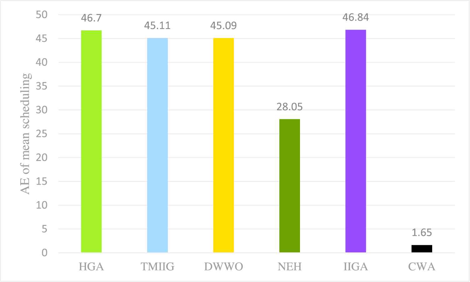
Average error (AE) of mean scheduling.
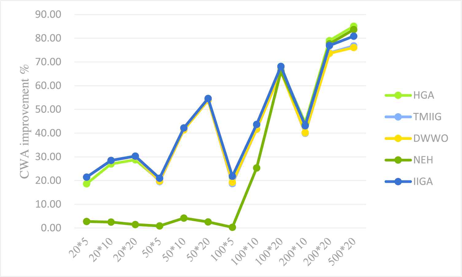
Improvement percentage (IP) of chaotic whale algorithm (CWA) based on the mean scheduling.
Table 13 shows the worst scheduling of Taillard benchmark instances. Comparing CWA with HGA [95], the results show that CWA is always better than HGA, including smaller or larger instances.
| Instance | n*m | Known Best | HGA | CWA | Instance | n*m | Known Best | HGA | CWA |
|---|---|---|---|---|---|---|---|---|---|
| Ta001 | 20*5 | 1278 | 1485 | 1278 | Ta061 | 100*5 | 5493 | 6594 | 5493 |
| Ta002 | 1359 | 1505 | 1359 | Ta062 | 5268 | 6469 | 5284 | ||
| Ta003 | 1081 | 1431 | 1081 | Ta063 | 5175 | 6320 | 5193 | ||
| Ta004 | 1293 | 1573 | 1293 | Ta064 | 5014 | 6198 | 5023 | ||
| Ta005 | 1235 | 1445 | 1235 | Ta065 | 5250 | 6397 | 5265 | ||
| Ta006 | 1195 | 1471 | 1195 | Ta066 | 5135 | 6296 | 5139 | ||
| Ta007 | 1239 | 1496 | 1239 | Ta067 | 5246 | 6460 | 5266 | ||
| Ta008 | 1206 | 1475 | 1206 | Ta068 | 5094 | 6359 | 5123 | ||
| Ta009 | 1230 | 1429 | 1230 | Ta069 | 5448 | 6561 | 5465 | ||
| Ta010 | 1108 | 1368 | 1108 | Ta070 | 5322 | 6592 | 5335 | ||
| Ta011 | 20*10 | 1582 | 1998 | 1622 | Ta071 | 100*10 | 5770 | 8230 | 5800 |
| Ta012 | 1659 | 2166 | 1692 | Ta072 | 5349 | 8101 | 5424 | ||
| Ta013 | 1496 | 1942 | 1534 | Ta073 | 5676 | 8215 | 5740 | ||
| Ta014 | 1377 | 1811 | 1434 | Ta074 | 5781 | 8505 | 5860 | ||
| Ta015 | 1419 | 1947 | 1467 | Ta075 | 5467 | 8096 | 5525 | ||
| Ta016 | 1397 | 1879 | 1539 | Ta076 | 5303 | 7947 | 5328 | ||
| Ta017 | 1484 | 1971 | 1504 | Ta077 | 5595 | 8081 | 5692 | ||
| Ta018 | 1538 | 2066 | 1571 | Ta078 | 5617 | 8105 | 5694 | ||
| Ta019 | 1593 | 1973 | 1646 | Ta079 | 5871 | 8349 | 5940 | ||
| Ta020 | 1591 | 2032 | 1674 | Ta080 | 5845 | 8340 | 5903 | ||
| Ta021 | 20*20 | 2297 | 2972 | 2362 | Ta081 | 100*20 | 6202 | 10932 | 6435 |
| Ta022 | 2099 | 2835 | 2160 | Ta082 | 6183 | 10847 | 6373 | ||
| Ta023 | 2326 | 2984 | 2372 | Ta083 | 6271 | 10821 | 6374 | ||
| Ta024 | 2223 | 2994 | 2316 | Ta084 | 6269 | 10797 | 6408 | ||
| Ta025 | 2291 | 3017 | 2338 | Ta085 | 6314 | 10777 | 6460 | ||
| Ta026 | 2226 | 2964 | 2263 | Ta086 | 6364 | 10853 | 6535 | ||
| Ta027 | 2273 | 3028 | 2353 | Ta087 | 6268 | 11031 | 6568 | ||
| Ta028 | 2200 | 2826 | 2267 | Ta088 | 6401 | 10992 | 6593 | ||
| Ta029 | 2237 | 3009 | 2299 | Ta089 | 6275 | 10963 | 6482 | ||
| Ta030 | 2178 | 2979 | 2246 | Ta090 | 6434 | 11067 | 6620 | ||
| Ta031 | 50*5 | 2724 | 3229 | 2735 | Ta091 | 200*10 | 10862 | 15916 | 10950 |
| Ta032 | 2834 | 3475 | 2838 | Ta092 | 10480 | 15764 | 10570 | ||
| Ta033 | 2621 | 3277 | 2624 | Ta093 | 10922 | 16026 | 11045 | ||
| Ta034 | 2751 | 3384 | 2762 | Ta094 | 10889 | 16111 | 10911 | ||
| Ta035 | 2863 | 3404 | 2864 | Ta095 | 10524 | 15829 | 10553 | ||
| Ta036 | 2829 | 3377 | 2835 | Ta096 | 10326 | 15731 | 10575 | ||
| Ta037 | 2725 | 3280 | 2725 | Ta097 | 10854 | 16029 | 10908 | ||
| Ta038 | 2683 | 3288 | 2705 | Ta098 | 10730 | 15933 | 10803 | ||
| Ta039 | 2552 | 3121 | 2577 | Ta099 | 10438 | 15759 | 10492 | ||
| Ta040 | 2782 | 3383 | 2814 | Ta100 | 10675 | 15934 | 10727 | ||
| Ta041 | 50*10 | 2991 | 4306 | 3054 | Ta101 | 200*20 | 11195 | 20458 | 11461 |
| Ta042 | 2867 | 4235 | 2923 | Ta102 | 11203 | 20889 | 11496 | ||
| Ta043 | 2839 | 4124 | 2953 | Ta103 | 11281 | 20636 | 11609 | ||
| Ta044 | 3063 | 4549 | 3071 | Ta104 | 11275 | 20753 | 11638 | ||
| Ta045 | 2976 | 4367 | 3051 | Ta105 | 11259 | 20601 | 11466 | ||
| Ta046 | 3006 | 4332 | 3083 | Ta106 | 11176 | 20780 | 11442 | ||
| Ta047 | 3093 | 4444 | 3165 | Ta107 | 11360 | 20915 | 11627 | ||
| Ta048 | 3037 | 4347 | 3076 | Ta108 | 11334 | 20814 | 11601 | ||
| Ta049 | 2897 | 4188 | 2965 | Ta109 | 11192 | 20757 | 11501 | ||
| Ta050 | 3065 | 4304 | 3120 | Ta110 | 11288 | 20712 | 11626 | ||
| Ta051 | 50*20 | 3850 | 6172 | 3984 | Ta111 | 500*20 | 26059 | 49580 | 26582 |
| Ta052 | 3704 | 5790 | 3859 | Ta112 | 26520 | 50354 | 27161 | ||
| Ta053 | 3640 | 5929 | 3831 | Ta113 | 26371 | 49399 | 26832 | ||
| Ta054 | 3720 | 5827 | 3864 | Ta114 | 26456 | 50004 | 26838 | ||
| Ta055 | 3610 | 5950 | 3794 | Ta115 | 26334 | 49847 | 26716 | ||
| Ta056 | 3681 | 5911 | 3803 | Ta116 | 26477 | 50046 | 27048 | ||
| Ta057 | 3704 | 6001 | 3798 | Ta117 | 26389 | 49591 | 26832 | ||
| Ta058 | 3691 | 5971 | 3880 | Ta118 | 26560 | 49942 | 27020 | ||
| Ta059 | 3743 | 5899 | 3826 | Ta119 | 26005 | 49697 | 26513 | ||
| Ta060 | 3756 | 5979 | 3922 | Ta120 | 26457 | 50002 | 26886 |
Comparison on Taillard benchmark based on the worst scheduling.
Figure 13 shows the improvement degree of CWA relative to HGA, and CWA is significantly improved. With the increment of instance size, the optimization degree of CWA increases, and reached 85.7% when the instance is 500*20. The experimental results show that the optimization of CWA is very successful.

Improvement percentage (IP) achieved by chaotic whale algorithm (CWA) for hybrid genetic algorithm (HGA) on the worst scheduling.
7. CONCLUSIONS AND FUTURE WORK
This paper proposed a new CWA which combined chaotic mapping, inserted local search, and cross selection operator. The chaotic map stabilizes the random factors in the algorithm and increases the stability and optimization of the algorithm. What's more, these strategies also make the algorithm avoid falling into the local optimum through local search with small probability and circular cross selection operator. NEH is used to initialize the population so that a better result can be obtained in the initialization stage. In the process of initializing population, LRV rule is used to transform the continuous search agent into discrete job sequence, which optimizes the rationality of job generation. The experimental results show that it is feasible to use chaos strategy to optimize whale algorithm.
Compared with other scheduling algorithms, CWA has other advantages, such as fewer variables to be adjusted, faster convergence speed, and more stability. Because the parameters have a great influence on the performance of the algorithm, its stability is improved when chaotic mapping is used to make the parameters tend to be controllable [106]. However, the algorithm still has uncertainty, which needs further optimization and improvement. In future, except the methods used in the current paper, some of the most presentative metaheuristic algorithms [107], such as BA [108–110], biogeography-based optimization (BBO) [111,112], ACO [113], cuckoo search (CS) [114,115], earthworm optimization algorithm (EWA) [116], elephant herding optimization (EHO) [117,118], moth search (MS) algorithm [119], firefly algorithm (FA) [120], ABC [121–123], harmony search (HS) [124], monarch butterfly optimization (MBO) [125,126], PSO [127,128], genetic programming [129], CS [84,130,131] and more recently, the KH algorithm [81,132–135].
In this paper, CWA is tested on Carlier, Reeves, Heller, and Taillard benchmarks. Since only these four groups of benchmark functions have been tested, another limitation is the lack of research on broader dimensions. But from the results of the experiment, the proposed CWA algorithm has better stability and optimization results. In the current work, we only apply CWA to PFSSP. In the future, the algorithm will be used to solve other engineering problems. We are ready to apply this algorithm to the differential distributed job shop scheduling system, and use it to study big data of ocean.
CONFLICTS OF INTEREST
The authors declare that they have no conflicts of interest.
AUTHORS' CONTRIBUTIONS
Conceptualization, J.L. and L.W.; methodology, L.G. and H.H.; software, Y.L. and L.W.; validation, J.L.; writing-original draft preparation, J.L. and C.L.; writing-review and editing, L.G.; All authors have read and agreed to the published version of the manuscript.
Funding Statement
This work was supported by the National Natural Science Foundation of China (No. 61977059).
ACKNOWLEDGMENTS
The authors would like to thank the anonymous reviewers and the editor for their careful reviews and constructive suggestions to help us improve the quality of this paper.
REFERENCES
Cite this article
TY  - JOUR
AU  - Jiang Li
AU  - Lihong Guo
AU  - Yan Li
AU  - Chang Liu
AU  - Lijuan Wang
AU  - Hui Hu
PY  - 2021
DA  - 2021/01/19
TI  - Enhancing Whale Optimization Algorithm with Chaotic Theory for Permutation Flow Shop Scheduling Problem
JO  - International Journal of Computational Intelligence Systems
SP  - 651
EP  - 675
VL  - 14
IS  - 1
SN  - 1875-6883
UR  - https://doi.org/10.2991/ijcis.d.210112.002
DO  - 10.2991/ijcis.d.210112.002
ID  - Li2021
ER  -