
Solving Logistics Distribution Center Location with Improved Cuckoo Search Algorithm
- DOI
- 10.2991/ijcis.d.201216.002How to use a DOI?
- Keywords
- Cuckoo search algorithm; Balanced-learning; The better fitness set; The better diversity set; Optimization algorithm
- Abstract
As a novel swarm intelligence optimization algorithm, cuckoo search (CS), has been successfully applied to solve various optimization problems. Despite its simplicity and efficiency, the CS is easy to suffer from the premature convergence and fall into local optimum. Although a lot of research has been done on the shortage of CS, learning mechanism has not been used to achieve the balance between exploitation and exploration. Based on this, a differential CS extension with balanced learning namely Cuckoo search algorithm with balanced-learning (O-BLM-CS) is proposed. Two sets, the better fitness set (FSL) and the better diversity set (DSL), are produced in the iterative process. Two excellent individuals are selected from two sets to participate in search process. The search ability is improved by learning their beneficial behaviors. The FSL and DSL learning factors are adaptively adjusted according to the individual at each generation, which improve the global search ability and search accuracy of the algorithm and effectively balance the contradiction between exploitation and exploration. The performance of O-BLM-CS algorithm is evaluated through eighteen benchmark functions with different characteristics and the logistics distribution center location problem. The results show that O-BLM-CS algorithm can achieve better balance between exploitation and exploration than other improved CS algorithms. It has strong competitiveness in solving both continuous and discrete optimization problems.
- Copyright
- © 2021 The Authors. Published by Atlantis Press B.V.
- Open Access
- This is an open access article distributed under the CC BY-NC 4.0 license (http://creativecommons.org/licenses/by-nc/4.0/).
NOMENCLATURE
| CS | Cuckoo search |
| Discover probability | |
| FSL | The better fitness set |
| DSL | The better diversity set |
| The minimum step size | |
| The maximum step size | |
| OBL | Opposition-based learning |
| NP | Population size |
| D | Dimension |
| R1 | Fitness learning factor |
| R2 | Diversity learning factor |
| T | Number of iterations |
| Best | The best fitness value |
| Mean | Average fitness value |
| Worst | The worst fitness value |
| STD | Standard deviation |
| Time | Running time |
1. INTRODUCTION
Lots of real-world problems can be converted to optimization problems, such as economic load dispatch, multi-robot path planning, wireless sensor networks, image segmentation, and radar applications. Optimization algorithms [1–3] are based on nature-inspired ideas with selecting the best alternative in a given objective function. In general, the optimization algorithms can be either a heuristic or a metaheuristic approach.
Rapid growth of the size and complexity of optimization problems implies a vital need for alternative optimization methods to the traditional mathematical optimization approaches [4]. Metaheuristic algorithms [5] have proved to be a viable solution to this challenge. Some of the well-known methods in this arena are genetic algorithms (GAs) [6–8], particle swarm optimization (PSO) [9–12], differential evolution (DE) [13–15], monarch butterfly optimization (MBO) [16–20], artificial bee colony (ABC) [21], earthworm optimization algorithm (EWA) [22], ant colony optimization (ACO) [23], chicken swarm optimization (CSO) [24], krill herd (KH) [25–27], firefly algorithm (FA) [28–33], simulated annealing (SA) [34], intelligent water drop (IWD) [35], water cycle algorithm (WCA) [36], moth search (MS) [37], monkey algorithm (MA) [38], evolutionary strategy (ES) [39], free search (FS) [40], probability-based incremental learning (PBIL) [41], biogeography-based optimization (BBO) [42–46], dragonfly algorithm (DA) [47], interior search algorithm (ISA) [48], brain storm optimization (BSO) [49,50], bat algorithm (BA) [51–59], stud GA (SGA) [60], harmony search (HS) [61–64], fireworks algorithm (FWA) [65], and cuckoo search (CS) [66–76].
The CS algorithm has been applied successfully to diverse fields since it was proposed by Yang and Deb [66]. A number of CS variants have been developed to improve the performance of the CS algorithm. These variants can be generally divided into five categories, which are population topology and multi-swarm techniques, parameter control, local search operator, hybrid methods with others algorithm, and novel learning schemes.
Yang and Deb [77] proposed a modified CS to solve practical engineering problems. Li et al. [78] enhanced the exploitation ability of the CS algorithm by using knowledge learning strategy. Gandomi et al. [79] developed a new CS algorithm to solve truss optimization problems. Kamoona et al. [80] proposed a novel enhanced cuckoo search (ECS) algorithm for image contrast enhancement, which proposed a new range of search space for the parameters of the local/global enhancement (LGE) transformation that need to be optimized. Yang et al. [81] proposed a novel modified CS algorithm named as NMCSA to solve optimal placement of actuators for active vibration control, which minimized control spillover effect and maximized the control force applied to the desired modes. Majumder et al. [82] proposed a hybrid discrete cuckoo search (HDCS) algorithm to minimize makespan for this scheduling problem. In HDCS, a modified lévy flight was proposed to transform a continuous position into a discrete schedule for generating a new solution. Ma et al. [83] proposed an improved dynamic self-adaption CS algorithm based on collaboration between subpopulations.
Although much effort has been made to enhance the performance of CS, many of the variants CS fail to improve the performance of CS algorithm on complicated problems. For example, some CS variants still cannot solve the global optimum for difficult problems involving many local optima. Meanwhile, some CS variants are able to increase population diversity, but they may face problems like slow convergence speed.
In this paper, we proposed an improved CS algorithm namely O-BLM-CS that adopts balanced-learning strategies. Although a lot of research has been done on the shortage of CS, learning mechanism has not been used to achieve the balance between exploitation and exploration. Based on this, in O-BLM-CS, the better fitness set (FSL) and the better diversity set (DSL), are produced in the iterative process. Two excellent individuals are selected from two sets to participate in search process. The search ability is improved by learning their beneficial behaviors. The FSL and DSL learning factors are adaptively adjusted according to the individual at each generation, which improve the global search ability and search accuracy of the algorithm and effectively balance the contradiction between exploitation and exploration. To verify the effectiveness of O-BLM-CS, we conducted comprehensive experiments on eighteen test functions and the logistics distribution center location problem. The experimental results show that O-BLM-CS performed better than other evolutionary algorithms in terms of the quality of the solution and convergence rate.
The main contributions of this study can be summarized as follows: (1) Fitness sorting learning mechanism (FSL) is introduced into individual updates, which improve the performance of algorithm exploitation. (2) Diversity sorting learning mechanism (DSL) is introduced into individual updates, which improve the performance of algorithm exploration. (3) Initialization with opposition-based learning model increases the chance for finding an individual close to the global best solution.
The remainder of this paper is organized as follows: Section 2 reviews the basic characteristics of CS, and then Section 3 describes balanced-learning model and O-BLM-CS algorithm steps. Benchmark problems and corresponding experimental results are given in Section 4. Finally, Section 5 concludes this paper and points out some future research directions.
2. CUCKOO SEARCH
The CS algorithm [66] is a nature-inspired evolutionary algorithm, which inspired by parasitism behavior of cuckoo species that lay eggs in other host birds. The algorithm is based on the obligate brood parasitic behavior found in some cuckoo nests by combining a model of this behavior with the principles of Lévy flights, which is a type of random walk with a heavy tail. CS is based on three idealized rules:
Each cuckoo lays one egg at a time, and places it in a randomly chosen nest.
The best nests with the highest quality eggs (solutions) will be carried over to the next generations.
The number of available host nests is fixed, and a host can discover an alien egg with the probability
The position of the number i nest are indicated by using D-dimensional vector, the offspring are produced by using Lévy flights (based on random walks). Lévy flight is performed as follows:
Algorithm 1: CS algorithm
(1) randomly initialize population of n host nests
(2) calculate fitness value for each solution in each nest
(3) while (stopping criterion is not meet do)
(4) for
(5) generate as new solution by using lévy flights;
(6) choose candidate solution;
(7) if
(8) replace with new solution;
(9) end if
(10) end for
(11) throw out a fraction
(12) for each abandoned nest
(13) for each
(14) generate solution
(15) if
(16) replace with new solution;
(17) end if
(18) end for
(19) end for
(20) rank the solution and find the current best
(21) end while
3. IMPROVED CS ALGORITHM
3.1. Initialization with Opposition-Based Learning Model
Tizhoosh [84] proposed an affective technique namely opposition-based learning (OBL) for enhancing various algorithms. The OBL transforms candidates from current search space to a new search space which add the opposition solutions of individual. The OBL increases the chance for finding an individual close to the global best solution by evaluating a solution and its opposition solution. When a solution x is evaluated, the opposite solution
In order to improve the search performance of CS, the OBL idea is introduced the CS to initialize the population in this paper. We split the population into two subpopulations (P1 and P2). The subpopulation P1 is generated by a random distribution. The subpopulation P2 is initialized in terms of OBL strategy. The two subpopulations are composed of one population after updating the solutions in the population, which can make the population size unchanged in the optimization process. Furthermore, the population is sorted by their fitness and located the best individual.
3.2. Individual Update with Balanced-Learning Model
The balance between exploitation and exploration is an important goal for optimization algorithm. In this second, two learning models, FSL and DSL, are introduced into the CS algorithm to balance the performance of CS algorithm in terms of exploitation and exploration.
Fitness sorting learning mechanism
In order to improve the performance of algorithm exploitation, FSL is introduced into individual updates. According to the fitness value of individuals, population is sorted in descending order in FSL. The individual with the smallest fitness value is the best. The new population after sorted by fitness is shown in the Figure 1, the first individual is the worst, and the n-th individual is the best. Xt is the current i-th individual.
Diversity sorting learning mechanism
In order to improve the performance of algorithm exploration, DSL is also introduced into individual updates. In DSL, according to the diversity of individuals, the individuals are sorted in descending order, in which the diversity
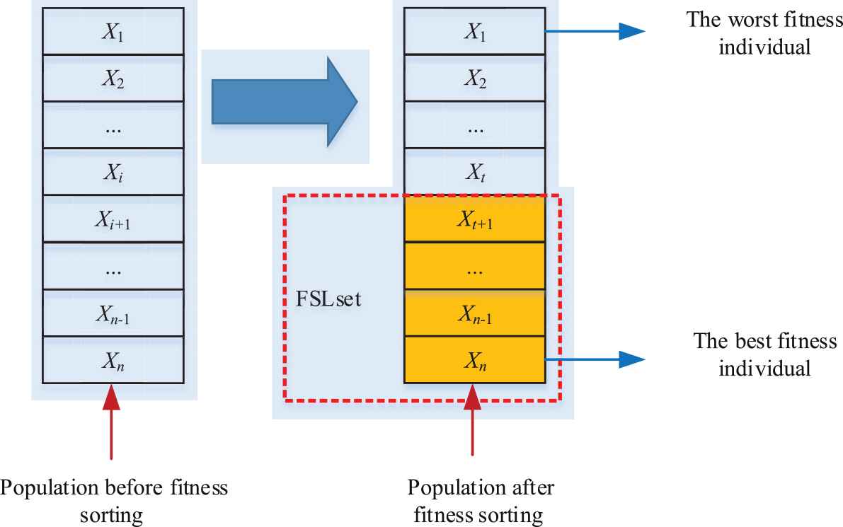
Sorting according to fitness.
The individual with the biggest diversity value is the best. In the new population after diversity sorting, as shown in the Figure 2, the first individual is the worst, and the n-th individual is the best. Xq is the current i-th individual.
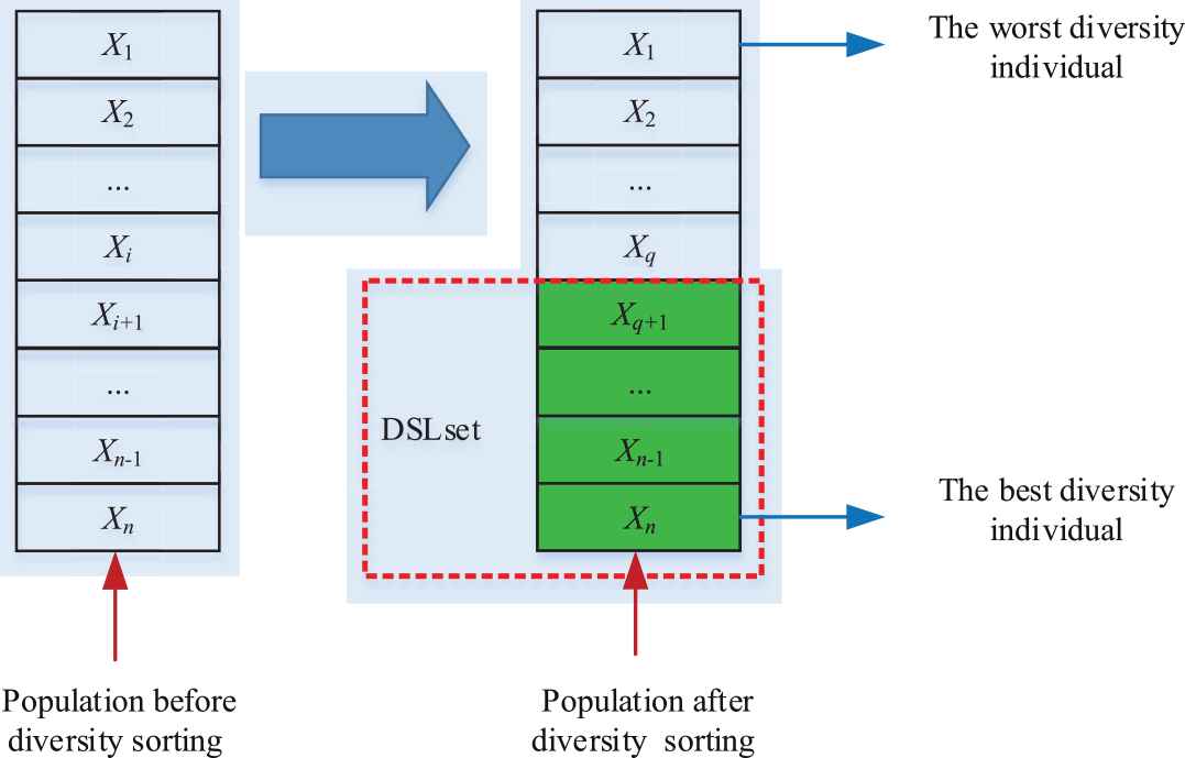
Sorting according to diversity.
where the
In the early stage of search, the algorithm tends to global search and needs a larger learning factor to improve the global search ability; in the later stage of search, the algorithm tends to local search and needs a smaller learning factor to improve the local search ability. The need for diversity changes as the number of iterations increases. Therefore, we adjust the learning factor R2 according to the evolution generations.
3.3. The Procedure Pseudo Code of O-BLM-CS Algorithm
FSL and DSL effectively balance the performance of CS algorithm in terms of exploitation and exploration. The structure of the CS algorithm with balance-Learning model algorithm (O-BLM-CS) can be described in Algorithm 2.
3.4. Analysis of Algorithm Complexity
The computational complexity of the O-BLM-CS algorithm is analyzed according to the steps in Algorithm 2. Let the population size and dimension are NP and D, respectively. Obviously, O-BLM-CS algorithm is just seven more steps, step (4) – (10), than the standard CS algorithm. In Algorithm 2, sorting by fitness in steps (4) has time complexity
Algorithm 2: O-BLM-CS algorithm
(1) initialize population in terms of opposition-based learning model
(2) calculate fitness value for each solution in each nest.
(3) for
(4) calculate the fitness values of individuals and sort according to fitness values.
(5) calculate the diversity of individuals and sort according to diversity.
(6) update the learning factor R2 of DSL according to Eq. (12).
(7) for
(8) update the learning factor R1 of FSL according to Eq. (12).
(9) randomly choose the better individual from the FSL set.
(10) randomly choose the better individual from the DSL set.
(11) generate
(12) choose candidate solution.
(13) if
(14) replace
(15) end if
(16) end for
(17) throw out a fraction
(18) for each abandoned nest
(19) for each
(20) generate solution
(21) if
(22) replace
(23) end if
(34) end for
(25) end for
(26) rank the solution and find the current best.
(27) end for
4. RESULTS
4.1. Optimization of Functions and Parameter Settings
In order to verify the performance of O-BLM-CS algorithm, eighteen different global optimization problems were tested. F1–F5 are unimodal functions, F6–F11 are multimodal functions with many local minima, F12–F14 are shifted unimodal functions, and F15–F18 are shifted multimodal functions. A brief description of these benchmark problems are described in Table 1. The experiments were carried out on a P4 Dual-core platform with a 1.75 GHz processor and 4 GB memory, running under the Windows 7.0 operating system. The algorithms were developed using MATLAB R2017a. The maximum number of iterations, population size, and the times of running were set to 30,000, 30, and 30, respectively. The probability that foreign eggs were found was
| Type | Function | Name | Search Range | Error Threshold | Global Optimum |
|---|---|---|---|---|---|
| Unimodal | F1 | Sphere | [−100, 100] | 10−6 | 0 |
| F2 | Rosenbrock | [−30, 30] | 10−6 | 0 | |
| F3 | Step | [−100, 100] | 10−6 | 0 | |
| F4 | Elliptic | [−100, 100] | 10−6 | 0 | |
| F5 | Schwefel 2.22 | [−10,10] | 10−6 | 0 | |
| Multimodal | F6 | Ackley | [−32,32] | 10−6 | 0 |
| F7 | Rastrigin | [−5.12, 5.12] | 10−6 | 0 | |
| F8 | Griewank | [−600, 600] | 10−6 | 0 | |
| F9 | Schwefel 2.26 | [−500, 500] | 10−6 | 0 | |
| F10 | Generalized Penalized 1 | [−50, 50] | 10−6 | 0 | |
| F11 | Generalized Penalized 2 | [−50, 50] | 10−6 | 0 | |
| Shifted unimodal | F12 | Shifted Sphere | [−100, 100] | 10−6 | −450 |
| F13 | Shifted Schwefels problem 1.2 | [−100, 100] | 10−6 | −450 | |
| F14 | Shifted rotated high conditioned elliptic function | [−100, 100] | 10−6 | −450 | |
| Shifted multimodal | F15 | Shifted Rosenbrock | [−100, 100] | 10−2 | 390 |
| F16 | Shifted rotated Ackleys | [−32, 32] | 10−2 | −140 | |
| F17 | Shifted rotated Griewanks | [−600, 600] | 10−2 | 0 | |
| F18 | Shifted rotated Rastrigin | [−5.12, 5.12] | 10−2 | −330 |
Brief description of eighteen functions.
4.2. Comparison with Other CS Variants and Rank-Based Analysis
This section focuses on some of the recent developments of CS algorithms that are directly related to our study. We compared O-BLM-CS with standard CS [66] and four improved CS variants: Chaos cuckoo search algorithm (CCS) [86], Gaussian disturbance cuckoo search algorithm (GCS) [87], Combination of cuckoo search and particle swarm optimization (CSPSO) [88], Orthogonal learning cuckoo search algorithm (OLCS) [67]. CCS [86] proposed a modified Chaos enhanced CS algorithm, which enhances initialized host nest location. GCS [87] is a cuckoo algorithm with Gaussian disturbance. CSPSO [88] is a kind of algorithm combining CS with PSO. OLCS [67] used a new search strategy with orthogonal learning to enhance the exploitation ability of CS algorithm. The parameter configurations of these algorithms are shown in Table 2 according to corresponding references. Eighteen benchmark functions on 30-dimensional and 50-dimensional are tested. The same parameters are set for all algorithms. Population size
| Algorithms | Parameter Configurations |
|---|---|
| CS [66] | |
| CCS [86] | |
| GCS [87] | |
| CSPSO [88] | |
| OLCS [67] | |
| O-BLM-CS |
The personal parameters of different algorithms.
| Func | CS | CCS | GCS | CSPSO | OLCS | O-BLM-CS |
|---|---|---|---|---|---|---|
| F1 | 2.02E-28±2.88E-27- | 3.53E-32±3.66E-31- | 4.34E-30±3.23E-31- | 5.32E-44±2.23E-44- | 2.34E-105±2.28E-100- | 0.00E+00±0.00E+00 |
| F2 | 2.55E+01±2.90E+00- | 4.99E-05±8.21E-05- | 2.95E-01±4.99E-01- | 8.98E+00±3.22E+00- | 1.33E-07±8.09E-07+ | 2.01E-07±2.33E-07 |
| F3 | 7.01E+00±0.11E+00- | 4.12E+00±2.80E+00- | 5.46E+00±2.22E+00- | 6.56E+00±3.11E+00- | 0.00E+00±0.00E+00+ | 4.51E-38±5.11E-38 |
| F4 | 9.00E-33±1.78E-32- | 6.98E-33±1.11E-33- | 4.09E-23±5.55E-23- | 3.56E-23±2.99E-23- | 2.24E-33±2.19E-33- | 4.65E-36±1.09E-36 |
| F5 | 2.99E-03±5.20E-03- | 2.87E-07±2.55E-07- | 3.89E-32±9.11E-48- | 3.78E-45±3.33E-45+ | 8.93E-48±1.45E-48+ | 1.90E-33±6.99E-32 |
| F6 | 7.23E-02±3.12E-01- | 8.91E-05±2.78E-06- | 0.05E-15±2.01E-012- | 5.52E-01±2.25E-01- | 2.41E-14±0.00E-00- | 0.66E-16±9.05E-16 |
| F7 | 2.88E+02±3.12E+02- | 2.10E-07±1.57E-07- | 3.34E-07±2.12E-07- | 3.00E+01±1.02E+01- | 0.00E-00±0.00E-00≈ | 0.00E+00±0.00E+00 |
| F8 | 8.23E-15±1.23E-15- | 3.02E-16±1.56E-16- | 5.88E-18±2.23E-17- | 5.11E-16±6.86E-16- | 0.00E-00±0.00E-00≈ | 0.00E+00±0.00E+00 |
| F9 | 7.11E+04±1.21E-08- | 6.12E+04±1.87E-08- | 1.66E+04±5.43E-08- | 2.67E+04±4.34E+04- | 3.43E+04±5.58E+04- | 5.09E+00±1.11E+00 |
| F10 | 2.87E+00±1.15E+00- | 5.12E-07±8.55E-07- | 3.23E-07±1.89 E-05- | 4.89E-06±2.00E-01- | 6.99E-08±3.09E-08- | 1.08E-10±4.55E-11 |
| F11 | 5.51E-03±4.46E-02- | 2.11E-23±5.16E-22- | 1.89E-22±3.04E-22- | 2.90E-04±6.00E-03- | 4.33E-29±1.09E-26- | 1.00E-29±3.09E-29 |
| F12 | 4.67E-29±4.47E-29- | 2.22E-29±4.34E-29+ | 3.65E-29±4.77 E-29- | 3.12E-29±3.48E-29- | 2.89E-29±6.23E-29+ | 3.08E-29±6.44E-29 |
| F13 | 2.90E-02±1.03E-01- | 4.56E-15±3.45E-16- | 3.24E-15±2.77E-16- | 3.26E-16±5.33E-16- | 3.77E-15±3.17E-11- | 1.84E-16±3.56E-16 |
| F14 | 3.39E+12±1.98E+12- | 3.56E+09±3.01E+09- | 2.11E+09±3.56E+09- | 2.45E+09±1.11E+01- | 3.56E+06±2.21E+06- | 2.66E+03±4.76E+03 |
| F15 | 8.87E+01±2.66E+00- | 0.73E+01±1.19E+01+ | 4.68E+01±3.57E+01- | 7.22E+01±2.11E+01- | 6.86E+01±4.57E+01- | 1.67E+01±3.76E+01 |
| F16 | 9.77E+03±1.21E+03- | 3.12E+03±2.85E+03- | 3.67E+03±2.8E+03- | 4.17E+04±1.11E+03- | 2.23E+03±3.88E+03+ | 3.98E+03±2.56E+03 |
| F17 | 8.88E-01±2.45E-02- | 4.61E-01±2.31E-01- | 6.45E-01±2.34E-01- | 1.23E-02±2.11E+02- | 0.00E+00±0.00E+00≈ | 0.00E+00±0.00E+00+ |
| F18 | 9.44E+01±2.46E+00- | 5.78E+01±2.67E+00- | 5.67E+01±2.28E+00- | 2.67E+02±4.99E+01- | 3.78E+01±1.66E+00- | 3.98E+00±0.88E+00 |
Mean values on eighteen benchmark functions for D = 30.
| Func | CS | CCS | GCS | CSPSO | OLCS | O-BLM-CS |
|---|---|---|---|---|---|---|
| F1 | 1.89E-12±4.05E-12- | 3.87E-16±1.66E-06- | 4.78E-19±5.07E-09- | 9.01E-18±2.45E-19- | 3.28E-28±8.01E-28- | 5.25E-30±6.97E-30 |
| F2 | 4.33E+01±8.01E+01- | 2.24E+01±1.45E+01- | 2.65E+01±1.23E+02- | 3.09E+01±1.90E-01- | 2.44E-01±1.59E-01- | 3.98E-02±1.34E-02 |
| F3 | 4.52E+02±1.21E+02- | 4.23E+01±1.02E+00- | 7.14E+01±4.56E+00- | 4.48E+01±2.01E+00- | 0.00E+00±0.00E-00+ | 2.40E+01±2.99E+01 |
| F4 | 4.87E-02±1.67E-02- | 2.11E-03±2.44E-02- | 2.56E-03±2.23E-02- | 1.34E-04±2.48E-04- | 6.05E-05±2.87E-05+ | 0.54E-04±6.83E-03 |
| F5 | 3.86E-01±5.29E-01- | 2.87E-02±1.22E-02- | 3.02E-27±1.10E-27- | 3.65E-27±1.48E-28- | 5.76E-26±3.78E-26- | 1.77E-28±3.56E-28 |
| F6 | 5.43E-01±3.03E-01- | 0.33E-02±3.78E-02- | 9.67E-07±4.87E-07+ | 9.31E-01±7.88E-02- | 2.90E-07±6.99E-07+ | 1.01E-06±5.65E-06 |
| F7 | 2.89E+04±1.92E+03- | 6.77E-01±1.89E-01- | 7.88E-06±3.91E-06+ | 3.82E+03±1.23E+03- | 0.00E-00±0.00E-00≈ | 0.00E-00±0.00E-00 |
| F8 | 3.98E-01±8.97E-01- | 3.44E-02±3.24E-02- | 4.17E-02±9.72E-02- | 6.16E-02±3.18E-02- | 0.00E-00±0.00E-00≈ | 0.00E+00±0.00E+00 |
| F9 | 9.02E+06±4.77E+06- | 3.56E+06±1.23E+01- | 7.00E+05±3.90E-00- | 3.63E+06±9.14E+06- | 5.66E+04±2.90E+04+ | 7.88E+04±2.19E+04 |
| F10 | 8.91E+00±3.27E+00- | 3.88E-05±1.67E-05- | 6.45E-07±4.21E-07- | 6.62E-07±2.90E-07- | 3.77E-07±3.23E-07- | 3.67E-07±2.11E-07 |
| F11 | 2.48E+01±2.98E+01- | 4.98E-03±9.01E-03- | 3.78E-20±4.87E-20- | 6.88E-01±3.98E-01- | 8.78E-26±1.78E-26- | 4.52E-26±2.89E-26 |
| F12 | 1.98E-02±3.88E-02- | 2.34E-12±1.67E-12- | 3.56E-20±1.32E-20- | 7.78E-20±6.12E-20- | 8.45E-21±3.55E-21- | 3.34E-21±1.12E-21 |
| F13 | 3.78E+00±1.03E+00- | 5.89E-10±1.69E-10- | 6.34E-10±4.23E-10- | 4.34E-10±8.25E-10+ | 7.34E-10±5.45E-09- | 2.22E-10±3.78E-10 |
| F14 | 5.84E+17±1.90E+17- | 2.67E+12±1.55 E+12- | 4.34E+12±4.11E+12- | 5.87E+12±6.66E+12- | 6.56E+08±4.99E+08+ | 4.89E+09±8.98E+09 |
| F15 | 5.87E+05±2.66E+00- | 3.73E+03±1.19E+03- | 7.68E+03±3.57E+03- | 5.22E+03±2.11E+03- | 3.86E+02±4.57E+01- | 2.67E+02±3.76E+02 |
| F16 | 6.03E+10±5.88E+10- | 4.56E+04±2.879E+04+ | 8.88E+04±1.91E+04- | 5.45E+05±4.76E+05- | 5.11E+04±2.11E+04+ | 6.61E+04±3.89E+04 |
| F17 | 6.88E+02±2.45E+01- | 3.66E+01±2.31E+02- | 4.45E+01±2.34E+02- | 4.23E+02±2.11E+02- | 0.00E+00±0.00E+00+ | 2.67E+01±5.89E+01 |
| F18 | 2.78E+02±8.11E+00- | 3.34E+02±1.12E+02- | 4.68E+02±1.10E+02- | 8.18E+03±2.14E+03- | 4.23E+02±1.23E+02- | 5.99E+01±6.42E+00 |
Mean values on eighteen benchmark functions for D = 50.
| Sign | CS | CCS | GCS | CSPSO | OLCS | MBL-CS |
|---|---|---|---|---|---|---|
| + | 0 | 2 | 0 | 1 | 5 | – |
| − | 18 | 16 | 18 | 17 | 10 | – |
| ≈ | 0 | 0 | 0 | 0 | 3 | – |
The ranking results of five algorithms for D = 30.
| Sign | CS | CCS | GCS | CSPSO | OLCS | MBL-CS |
|---|---|---|---|---|---|---|
| + | 0 | 1 | 2 | 1 | 7 | – |
| − | 18 | 17 | 16 | 17 | 9 | – |
| ≈ | 0 | 0 | 0 | 0 | 2 | – |
The ranking results of five algorithms for D = 50.
The average (Mean) and standard deviation (STD) with 30-dimensionnal and 50-dimensionnal are reported in Tables 3 and 4. Wilcoxon signed-rank test between O-BLM-CS and five algorithms (CS, CCS, GCS, OLCS, and CSPSO) at 30-dimensionnal and 50-dimensionnal was conducted in Tables 5 and 6 in which signs “+,” “−,” and “≈” indicate that the performance of O-BLM-CS is better than, less than and similar to other competitor.
The optimization results for 30-dimensional (30-D): From Table 3, O-BLM-CS can get global optima on functions F1, F7, F8, and F17 with 100% robustness. OLCS can get global optima on functions F3, F7, F8, and F17. For unimodal functions F1–F5, O-BLM-CS achieves higher accuracy than other algorithms on functions F1 and F4. OLCS achieves higher accuracy than other algorithms on functions F2, F3, and F5. O-BLM-CS is only inferior to OLCS on F2 and F3. For multimodal problems F6–F11, O-BLM-CS was significantly better than other algorithms on all functions. OLCS can get global optima on functions F7 and F8. For the shifted unimodal functions, O-BLM-CS achieves higher accuracy than other algorithms on F13 and F14. For the shifted multimodal functions F16 and F17, for F15, CCS is the best, for F16, OLCS is the best. Therefore, these statistical tests confirmed that O-BLM-CS algorithm with balanced-learning have better overall performance than other tested competitors. The ranking results of five algorithms are summed in Table 5.
The optimization results for 50-dimensional (50-D): From Table 3, for F7 and F8, only O-BLM-CS and OLCS can get global optima. For F3, F14, and F17, OLCS can get global optima. For unimodal functions F1–F5, O-BLM-CS is the best on F1, F2, and F5. OLCS achieves higher accuracy than other algorithms on F3. For multimodal problems F6–F11, O-BLM-CS achieves higher accuracy than other algorithms on F10 and F11. OLCS is the best on F6. For the shifted unimodal functions, O-BLM-CS achieves higher accuracy than other algorithms on F15 and F18. OLCS is the best on F14 and F17. O-BLM-CS is only inferior to OLCS on F3, F6, F9, F14, and F17. For F13, CSPSO is the best, and for F16, CCS is the best. Therefore, these statistical tests confirmed that O-BLM-CS algorithm with balanced-learning have better overall performance than other tested competitors. The Wilcoxon signed-rank test results are summed in Table 6. We can see that the O-BLM-CS optimization algorithms explore a larger search space than other algorithms. Altogether, the obtained results on 30-dimensional and 50-dimensional reveal that O-BLM-CS provides appropriate level of exploration and exploitation trade-off over the considered problems.
The performance ranking of six algorithms is listed in Tables 7–10 based on the Wilcoxon test. When their performances are same, algorithms are put in the same rank in competition ranking. For
| Algorithm | F1 | F2 | F3 | F4 | F5 | F6 | F7 | F8 | F9 |
|---|---|---|---|---|---|---|---|---|---|
| CS | 6 | 6 | 6 | 4 | 6 | 5 | 6 | 6 | 6 |
| CCS | 4 | 3 | 3 | 3 | 5 | 4 | 3 | 4 | 5 |
| GCS | 5 | 4 | 4 | 6 | 4 | 2 | 4 | 3 | 2 |
| CSPSO | 3 | 5 | 5 | 5 | 2 | 6 | 5 | 5 | 3 |
| OLCS | 2 | 1 | 1 | 2 | 1 | 3 | 1.5 | 1.5 | 4 |
| O-BLM-CS | 1 | 2 | 2 | 1 | 3 | 1 | 1.5 | 1.5 | 1 |
Rank table for the mean values of 30-dimensional cases on F1–F9.
| Algorithm | F10 | F11 | F12 | F13 | F14 | F15 | F16 | F17 | F18 |
|---|---|---|---|---|---|---|---|---|---|
| CS | 6 | 6 | 6 | 6 | 6 | 6 | 5 | 6 | 5 |
| CCS | 4 | 3 | 1 | 5 | 2 | 1 | 2 | 5 | 4 |
| GCS | 3 | 4 | 5 | 3 | 3 | 3 | 3 | 4 | 3 |
| CSPSO | 5 | 5 | 4 | 2 | 5 | 5 | 6 | 3 | 6 |
| OLCS | 2 | 2 | 2 | 4 | 4 | 4 | 1 | 1.5 | 2 |
| O-BLM-CS | 1 | 1 | 3 | 1 | 1 | 2 | 4 | 1.5 | 1 |
Rank table for the mean values of 30-dimensional cases on F10–F18.
| Algorithm | F1 | F2 | F3 | F4 | F5 | F6 | F7 | F8 | F9 |
|---|---|---|---|---|---|---|---|---|---|
| CS | 6 | 6 | 6 | 8 | 6 | 5 | 6 | 6 | 6 |
| CCS | 5 | 3 | 3 | 6 | 5 | 4 | 4 | 3 | 3 |
| GCS | 3 | 4 | 5 | 7 | 2 | 3 | 3 | 4 | 5 |
| CSPSO | 4 | 5 | 4 | 4 | 3 | 6 | 5 | 5 | 4 |
| OLCS | 2 | 2 | 1 | 1 | 4 | 1 | 1.5 | 1.5 | 1 |
| O-BLM-CS | 1 | 1 | 2 | 2 | 1 | 2 | 1.5 | 1.5 | 2 |
Rank table for the mean values of 50-dimensional cases on F1–F9.
| Algorithm | F10 | F11 | F12 | F13 | F14 | F15 | F16 | F17 | F18 |
|---|---|---|---|---|---|---|---|---|---|
| CS | 6 | 6 | 6 | 6 | 6 | 6 | 6 | 6 | 2 |
| CCS | 5 | 4 | 5 | 3 | 3 | 3 | 1 | 3 | 3 |
| GCS | 3 | 3 | 3 | 4 | 4 | 5 | 4 | 5 | 5 |
| CSPSO | 4 | 5 | 4 | 1 | 5 | 4 | 5 | 4 | 6 |
| OLCS | 2 | 2 | 2 | 5 | 1 | 2 | 3 | 1 | 4 |
| O-BLM-CS | 1 | 1 | 1 | 2 | 2 | 1 | 2 | 2 | 1 |
Rank table for the mean values of 50-dimensional cases on F10–F18.
| Dim | Rank | Algorithms |
|||||
|---|---|---|---|---|---|---|---|
| CS | CCS | GCS | CSPSO | OLCS | O-BLM-CS | ||
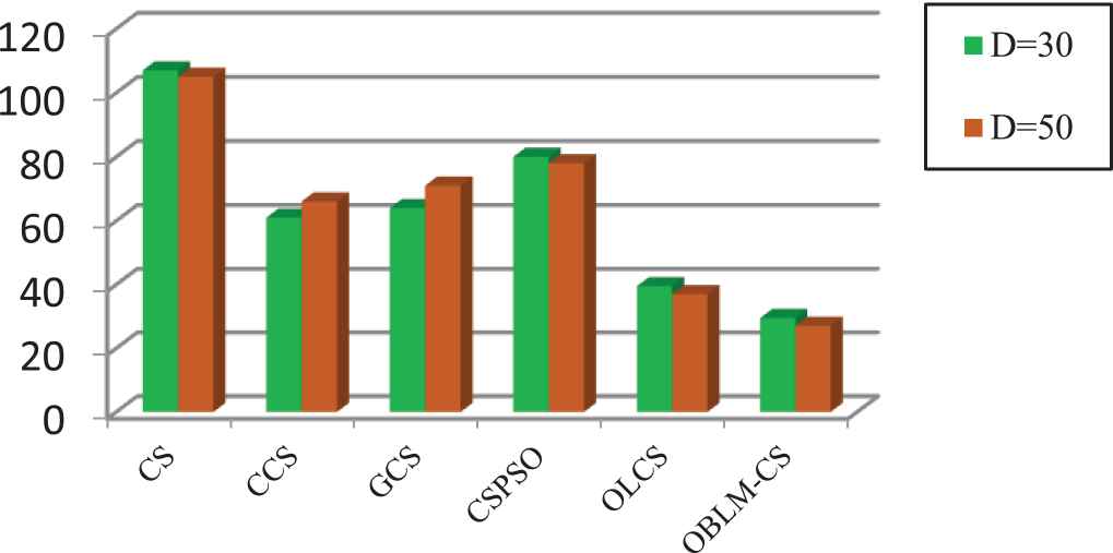
| 30 | Total rank | 107 | 61 | 64 | 80 | 39.5 | 29.5 |
| Final rank | 6 | 3 | 4 | 5 | 2 | 1 | |
| 50 | Total rank | 105 | 66 | 71 | 78 | 37 | 27 |
| Final rank | 6 | 3 | 4 | 5 | 2 | 1 | |
Total rank and final rank on F1–F18.
The convergence graphs of different algorithms on unimodal and multimodal functions (D = 30).
It can be observed From Table 11 that O-BLM-CS has the best total rank at
In order to verify the convergence performance of the O-BLM-CS, the convergence progress on six benchmark functions (F1, F2, F6, F7, F15, and F19) are shown in Figure 4. From Figure 4, O-BLM-CS algorithms converged to the specified error threshold on F1, F7, and F17. For F1, OLCS obtains faster convergence rate than CS, CCS, GCS, and CSPSO. The convergence curves of F2, F6, and F15 are similar, almost all algorithms have trapped into evolution stagnation. All algorithms cannot get the global minimum. For F17, O-BLM-CS and OLCS can get the global minimum and a part of compared algorithms (CS, CCS, GCS, and CSPSO) have trapped into the evolution stagnation. It is worth mentioning that although convergence rate of OLCS is close to O-BLM-CS, the convergence speed of O-BLM-CS is much faster than the convergence speed of OLCS. For all these functions, O-BLM-CS can get the fastest convergence speed except F15. F6 and F15 are similar, almost all algorithms have trapped into evolution stagnation. For F7 and F17, O-BLM-CS algorithms are able to find the global optimum with about 50,000 FES.
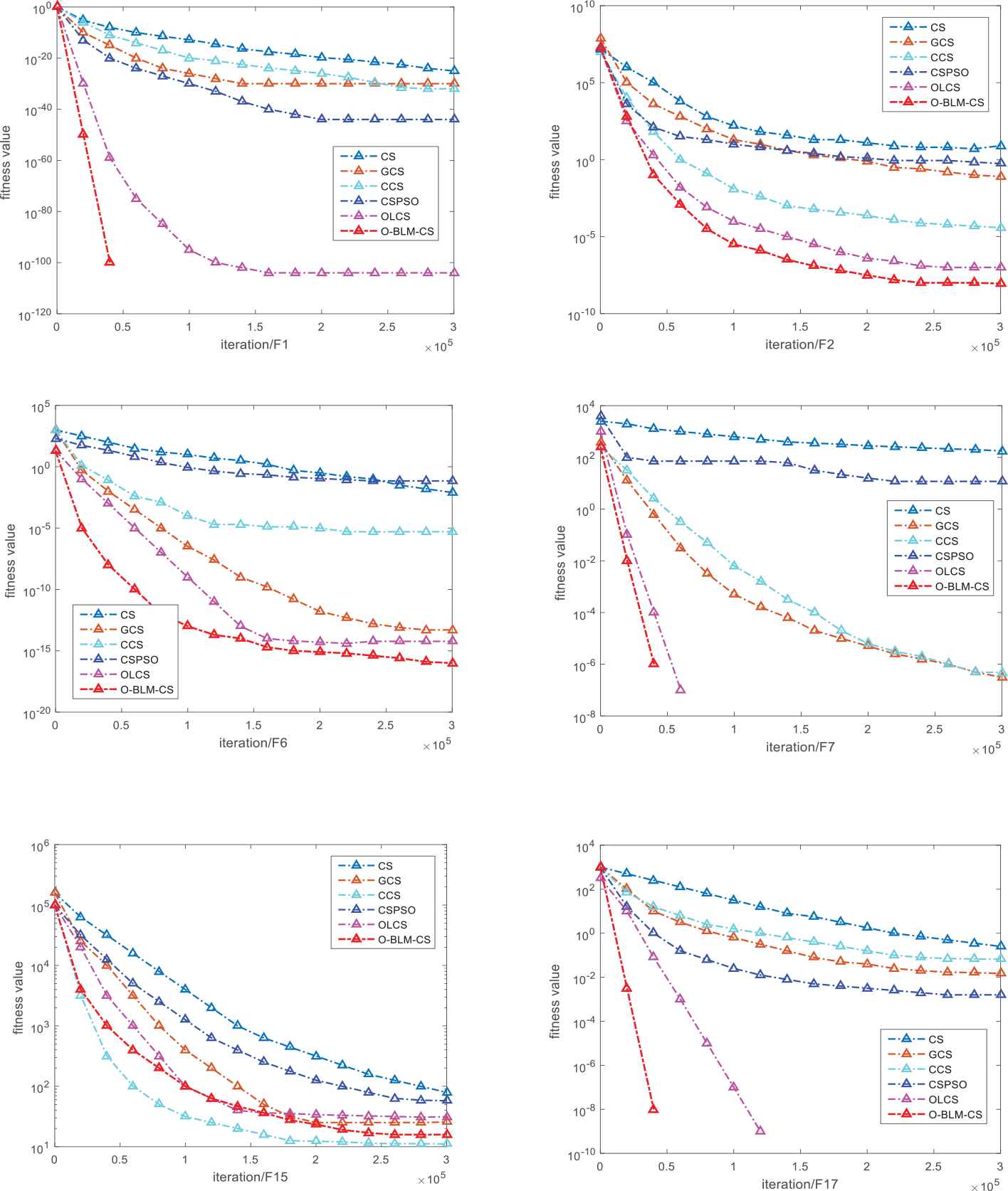
The convergence graphs of different algorithms on unimodal and multimodal functions (D = 30).
4.3. Application in the Problem of Logistics Distribution Center Location
4.3.1. Problem description
The distribution center is the most important hardware facility for logistics distribution center in the logistics system. All the logistics activities are almost entirely carried out with the distribution center. The positioning of the distribution center almost determines the cost required for the distribution business, which is a very important node in supply chain. Logistics distribution center location problem belongs to the research problem of the logistics management strategy level. Distribution center location includes single distribution center location and multiple distribution center location. Multiple distribution center location is discussed in this paper. The logistics distribution center location selects a certain number of locations in a number of known sites, which minimize the total cost of forming the logics network. This type of problem with the nature of NP-hard problems is a nonlinear model with more complex constraints and non-smooth characteristics. The problem can be described as: m cargo distribution center are search in n demand point, so that the distance between m searched distribution centers and other n cargo demand points is the shortest. The constraint conditions are as follows:
The supply of goods in the distribution center can meet the requirements of the cargo demand point;
The goods required for a cargo demand point can only be provided by one distribution center;
The cost of transporting the goods to the distribution center is not considered.
According to the above assumptions, the mathematical model of the problem for logistics distribution center location can be described as:
4.3.2. Analysis of experimental results
In this section, there is a logistics network with 40 demand points. The geographical position coordinates and demands were shown in Table 12. The maximum number of iterations
| No | Coordinates |
Demand | No | Coordinates |
Demand | No | Coordinates |
Demand | No | Coordinates |
Demand | ||||
|---|---|---|---|---|---|---|---|---|---|---|---|---|---|---|---|
| x | y | x | y | x | y | x | y | ||||||||
| 1 | 97 | 28 | 94 | 11 | 91 | 96 | 85 | 21 | 111 | 117 | 92 | 31 | 125 | 66 | 45 |
| 2 | 100 | 56 | 11 | 12 | 39 | 90 | 54 | 22 | 63 | 42 | 99 | 32 | 169 | 49 | 98 |
| 3 | 45 | 67 | 50 | 13 | 50 | 101 | 25 | 23 | 67 | 105 | 98 | 33 | 31 | 188 | 31 |
| 4 | 150 | 197 | 88 | 14 | 67 | 66 | 87 | 24 | 160 | 156 | 88 | 34 | 86 | 42 | 91 |
| 5 | 105 | 48 | 80 | 15 | 157 | 54 | 66 | 25 | 100 | 125 | 47 | 35 | 90 | 21 | 79 |
| 6 | 24 | 158 | 29 | 16 | 104 | 35 | 82 | 26 | 35 | 48 | 47 | 36 | 46 | 53 | 47 |
| 7 | 88 | 61 | 93 | 17 | 169 | 95 | 48 | 27 | 143 | 172 | 34 | 37 | 62 | 30 | 84 |
| 8 | 55 | 105 | 10 | 18 | 48 | 39 | 78 | 28 | 94 | 56 | 33 | 38 | 163 | 176 | 52 |
| 9 | 120 | 120 | 18 | 19 | 115 | 61 | 16 | 29 | 57 | 73 | 43 | 39 | 190 | 141 | 10 |
| 10 | 43 | 105 | 38 | 20 | 154 | 174 | 49 | 30 | 25 | 127 | 100 | 40 | 170 | 30 | 77 |
The geographical position coordinates and demands.
For the first set of experiments, the effectiveness of the O-BLM-CS is verified by comparing CS algorithms. 4, 6, and 10 points were selected as the address of the distribution center to minimize the sum of all costs in this experiment. When the number of iterations
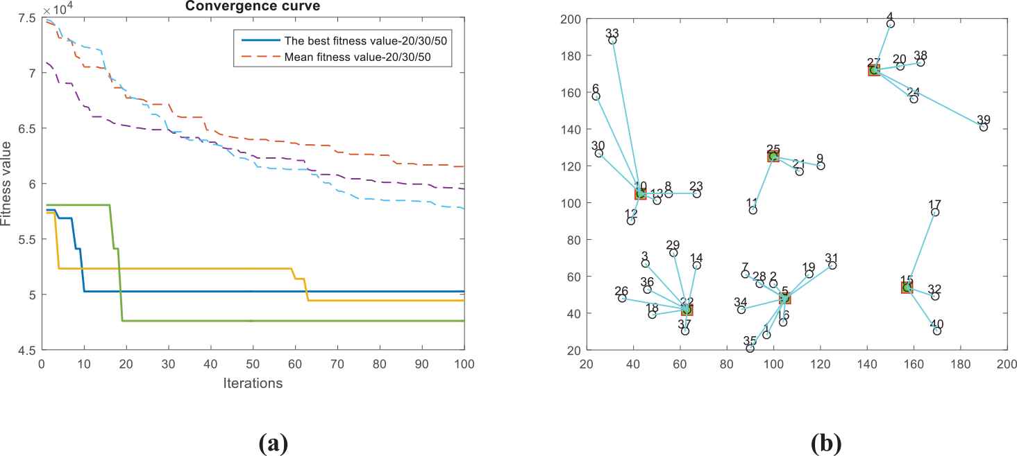
Convergence curves and optimal distribution centers scheme for the cuckoo search (CS) algorithm in 6 distribution centers (T = 100).

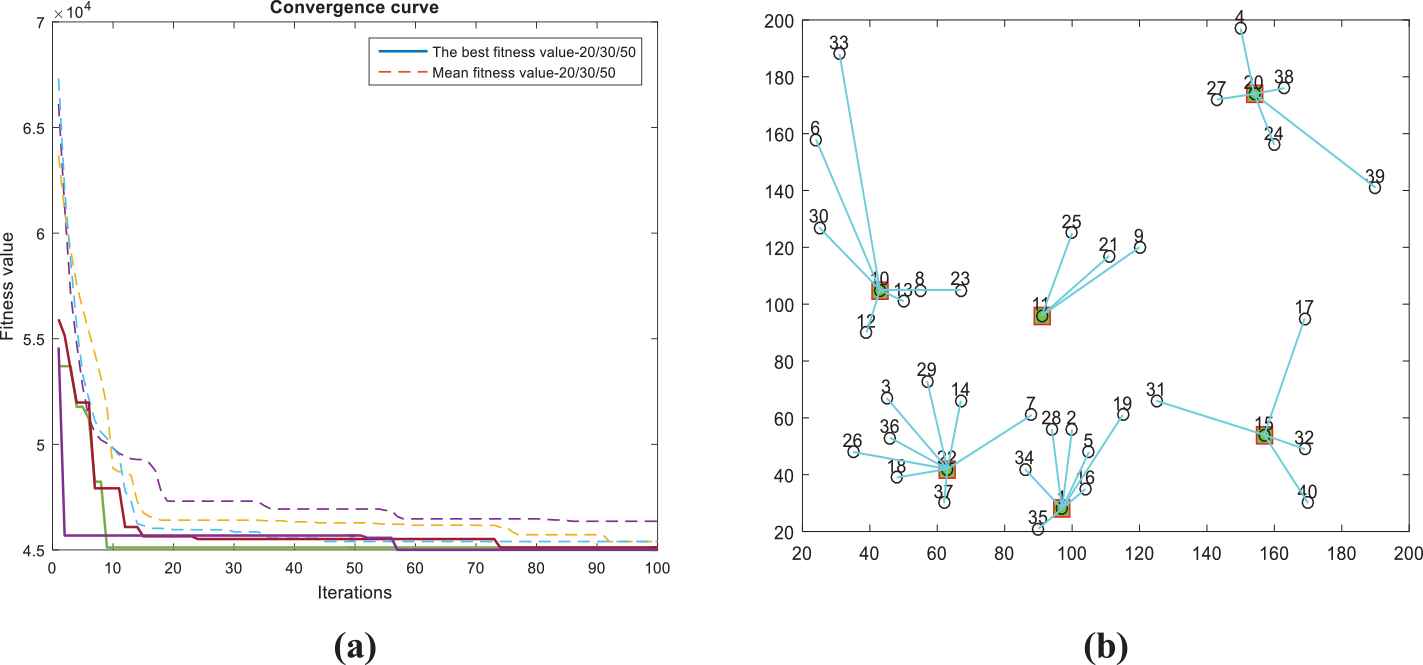
Convergence curves and optimal distribution centers schemefor the cuckoo search (CS) algorithm in 4 distribution center (T = 500).

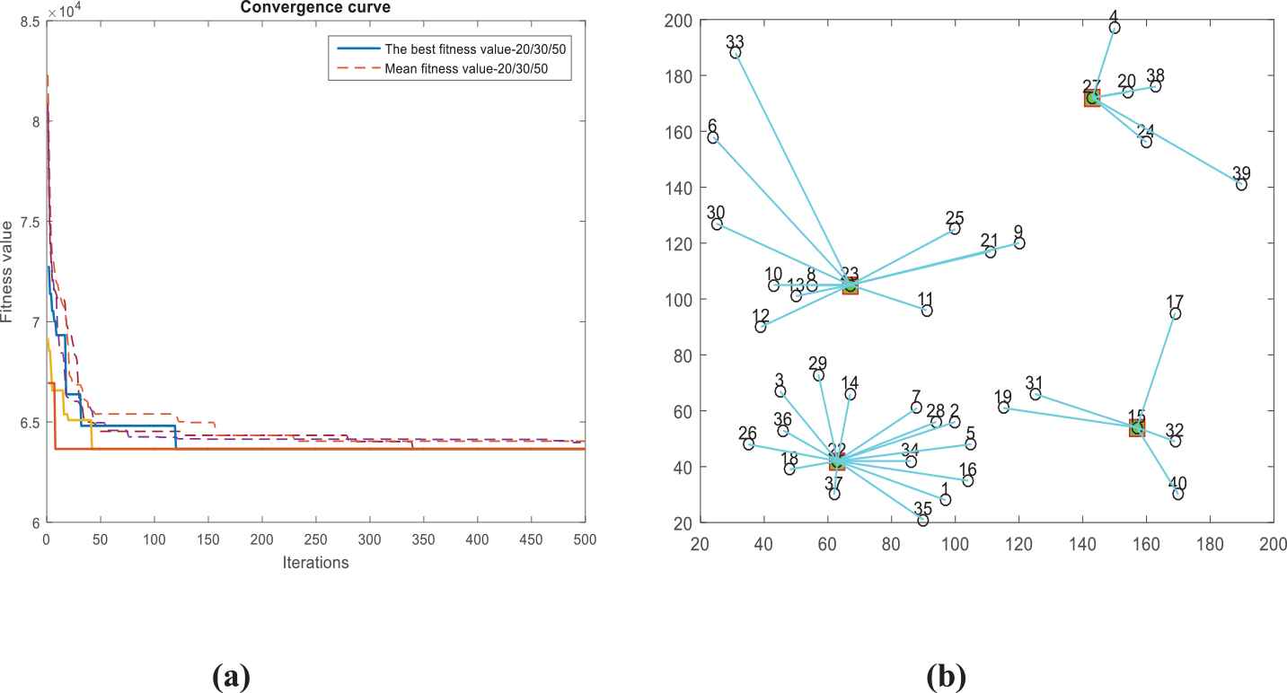
Convergence curves and optimal distribution centers scheme for the (CS) algorithm in 6 distribution centers (T = 500).

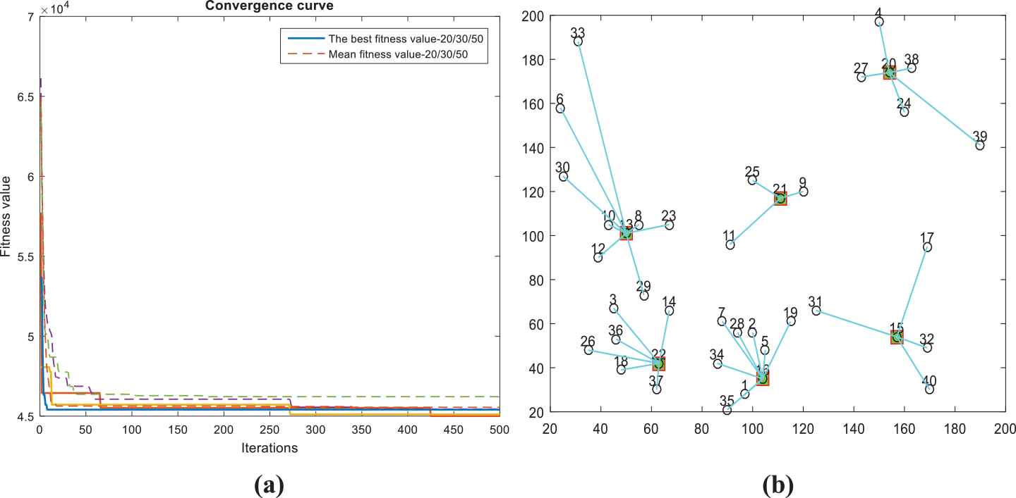
Convergence curves and optimal distribution centers scheme for the cuckoo search (CS) algorithm in 10 distribution centers (T = 500).
It can be seen from Figure 5a, the optimal convergence curve of CS in 6 distribution centers for 100 iteratings can converge at 20 iterations, but the average convergence curve is not converged. The optimal distribution, average distribution, and the worst distribution cost obtained in 6 distribution centers for 100 iterations are 4.7345E04, 5.9312E04, and 6.8017E04, respectively. From Figure 6a, the optimal convergence curve of CS in 4 distribution centers for 500 iterations can converge at 100 iterations, the average convergence curve can converge at 250 iterations. The optimal distribution, average distribution, and the worst distribution cost obtained in 4 distribution centers for 500 iteratings are 6.5268E04, 7.4188E04, and 7.7992E04, respectively. From Figure 7a, the optimal convergence curve of CS in 6 distribution centers for 500 iterations can converge at 50 iterations, the average convergence curve can converge at 200 iterations. The optimal distribution, average distribution, and the worst distribution cost obtained in 6 distribution centers for 500 iterations are 4.7128E04, 5.399E04, and 5.6927E04, respectively. From Figure 8, the optimal convergence curve of CS in 10 distribution centers for 500 iterations can converge at 300 iterations, the average convergence curve is not converged. The optimal distribution, average distribution, and the worst distribution cost obtained in 10 distribution centers for 500 iterations are 3.0265E04, 3.4765E04, and 3.8255E04, respectively.
Table 13 shows distribution range 100 iterations for 6 distribution centers in 40 cities, and Tables 14–16 show distribution range 500 iterations for 4, 6, and 10 distribution centers, respectively. From Tables 13–16, the optimal distribution center points found by CS in 6 distribution centers for 100 iterations is (10, 25, 27, 22, 5, 15). The optimal distribution center points in 4, 6, and 10 distribution centers for 500 iterations are (8, 22, 27, 15), (30, 23, 20, 18, 1, 15), and (11, 21, 20, 14, 8, 30, 5, 22, 1, 15), respectively.
| Distribution Center | Distribution Scope |
|---|---|
| 10 | 33, 6, 30, 12, 13, 8, 23 |
| 25 | 11, 21, 9 |
| 27 | 4, 38, 20, 24, 39 |
| 22 | 14, 29, 3, 36, 26, 18, 37 |
| 5 | 7, 28, 2, 1, 25, 16, 19, 34, 35 |
| 15 | 31, 17, 32, 40 |
The distribution scheme for the cuckoo search (CS) algorithm in 6 distribution center (T = 100).
| Distribution Center | Distribution Scope |
|---|---|
| 8 | 33, 6, 30, 10, 12, 13, 23, 25, 21, 11 |
| 22 | 26, 36, 3, 29, 14, 18, 37, 7, 28, 2, 34, 5, 16, 1, 35 |
| 27 | 4, 9, 20, 24, 38, 39 |
| 15 | 19, 31, 17, 32, 40 |
The distribution scheme for the cuckoo search (CS) algorithm in 4 distribution center (T = 500).
| Distribution Center | Distribution Scope |
|---|---|
| 30 | 33, 6 |
| 23 | 11, 25, 9, 21, 10, 13, 12, 8, 29 |
| 20 | 4, 27, 38, 24, 39 |
| 18 | 14, 3, 36, 26, 37, 22 |
| 1 | 28, 7, 34, 2, 5, 16, 35 |
| 15 | 31, 17, 32, 40 |
The distribution scheme for the cuckoo search (CS) algorithm in 6 distribution centers (T = 500).
| Distribution Center | Distribution Scope |
|---|---|
| 11 | - |
| 21 | 25, 9 |
| 20 | 4, 27, 38, 24, 39 |
| 14 | 3, 29 |
| 8 | 12, 10, 13, 23 |
| 30 | 6, 33 |
| 5 | 7, 28, 2, 19, 31 |
| 22 | 36, 26, 18, 37, 7 |
| 1 | 34, 35 |
| 15 | 17, 32, 40 |
The distribution scheme for the cuckoo search (CS) algorithm in 10 distribution centers (T = 500).
For the second set of experiments, the O-BLM-CS algorithm is run 20, 30, and 50 times independently in 40 cities 4, 6, 10 distribution center. When the number of iterations
Convergence curves and optimal distribution centers scheme for the O-BLM-CS algorithm in 6 distribution centers (T = 100).
Convergence curves and optimal distribution centers scheme for the O-BLM-CS algorithm in 4 distribution centers (T = 500).
Convergence curves and optimal distribution centers scheme for the O-BLM-CS algorithm in 6 distribution centers (T = 500).
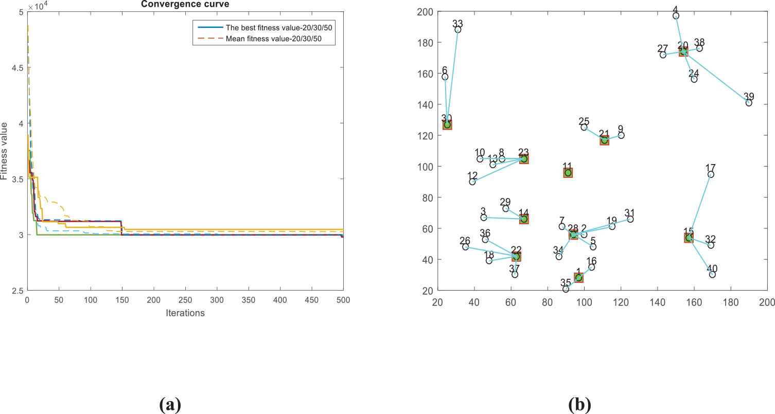
Convergence curves and optimal distribution centers scheme for the O-BLM-CS algorithm in 10 distribution centers (T = 500).
| Distribution Center | Distribution Scope |
|---|---|
| 10 | 33, 6, 30, 12, 13, 8, 23 |
| 11 | 25, 21, 9 |
| 20 | 4, 38, 27, 24, 39 |
| 22 | 14, 29, 3, 36, 26, 18, 37, 7 |
| 1 | 28, 2, 5, 16, 34, 35, 19 |
| 15 | 31, 17, 32, 40 |
The distribution scheme for the O-BLM-CS algorithm in 6 distribution centers (T = 100).
| Distribution Center | Distribution Scope |
|---|---|
| 23 | 33, 6, 30, 10, 12, 13, 8, 25, 21, 11, 9 |
| 22 | 26, 36, 3, 29, 14, 18, 37, 7, 28, 2, 34, 5, 16, 1, 35 |
| 27 | 4, 9, 20, 24, 38, 39 |
| 15 | 19, 31, 17, 32, 40 |
The distribution scheme for the O-BLM-CS algorithm in 4 distribution centers (T = 500).
| Distribution Center | Distribution Scope |
|---|---|
| 13 | 33, 6, 30, 12, 10, 8, 23, 29 |
| 21 | 11, 25, 9 |
| 20 | 4, 27, 38, 24, 39 |
| 22 | 14, 3, 36, 26, 37, 18 |
| 16 | 28, 7, 34, 2, 5, 19, 35, 1 |
| 15 | 31, 17, 32, 40 |
The distribution scheme for the O-BLM-CS algorithm in 6 distribution centers (T = 500).
| Distribution Center | Distribution Scope |
|---|---|
| 11 | - |
| 21 | 25, 9 |
| 20 | 4, 27, 38, 24, 39 |
| 14 | 3, 29 |
| 8 | 12, 10, 13, 23 |
| 30 | 6, 33 |
| 28 | 7, 5, 2, 19, 31, 34 |
| 22 | 36, 26, 18, 37, |
| 1 | 35, 16 |
| 15 | 17, 32, 40 |
The distribution scheme for the O-BLM-CS algorithm in 10 distribution centers (T = 500).
Figure 9 shows that the optimal convergence curve of O-BLM-CS in 6 distribution centers for 100 iteratings can converge at 10 iterations, the average convergence curve can converge at 15 iterations. The optimal distribution, average distribution, and the worst distribution cost obtained in 6 distribution centers for 100 iterations are 4.5027E04, 4.6082E04, and 4.7492E04, respectively. From Figure 10a, the optimal convergence curve of O-BLM-CS in 4 distribution centers for 500 iteratings can converge at 20 iterations, the average convergence curve can converge at 15 iterations. The optimal distribution, average distribution, and the worst distribution cost obtained in 4 distribution centers for 500 iterations are 6.3813E04, 6.4194E04, and 6.4231E04, respectively. From Figure 11a, the optimal convergence curve of O-BLM-CS in 6 distribution centers for 500 iterations can converge at 5 iterations, the average convergence curve can converge at 50 iterations. The optimal distribution, average distribution, and the worst distribution cost obtained in 6 distribution centers for 500 iterations are 4.5021E04, 4.5181E04, and 4.6023E04, respectively. From Figure 12a, the optimal convergence curve of O-BLM-CS in 10 distribution centers for 500 iterations can converge at 10 iterations, the average convergence curve can converge at 10 iterations. The optimal distribution, average distribution and the worst distribution cost obtained in 10 distribution centers for 500 iterations iterations are 2.8234E04, 3.0618E04, and 3.1886E04, respectively.
Table 17 shows distribution ranges 100 iterations for 6 distribution centers in 40 cities, and Tables 18–20 show distribution ranges 500 iterations for 4, 6, and 10 distribution centers, respectively. From Tables 17–20, the optimal distribution center points found by O-BLM-CS algorithm in 6 distribution centers for 100 iterations is (10, 11, 20, 22, 1, 5). The optimal distribution center points in 4, 6, and 10 distribution centers for 500 iteratings are (23, 22, 27, 15), (12, 21, 20, 22, 16, 15), and (11, 21, 20, 14, 8, 30, 28, 22, 1, 15), respectively.
It can be seen from Figures 5 and 9, logistics distribution location strategy of O-BLM-CS in 6 distribution centers at 100 iterations for 10 distribution centers is better than CS in both the optimal convergence curve and the average convergence curve. The average convergence curve of O-BLM-CS can converge at 15 iterations, but CS does not converge to the optimal solution. It can be seen from Figures 6a and 10a, the average convergence curve of O-BLM-CS in 4 distribution centers at 500 iterations can converge at 15 iterations. the average convergence curve of CS can converge at 250 iterations, which in include O-BLM-CS is far superior to CS for terms of convergence speed. Although the CS algorithm can converge, it has a lot of noise for the average convergence curve. For 500 iterations and 10 distributions, CS converges only at 200 iterations, while O-BLM-CS converges to the optimal solution at 50 iterations. It is worth mentioning that CS does not converge to the optimal solution at 100 iterations for 10 distributions. O-BLM-CS converges to the optimal solution at just 10 iterations. It indicates that O-BLM-CS has fast speed and high solution accuracy, which effectively reduces the cost of logistics distribution. In addition, the results of STD indicate that the O-BLM-CS has a better robustness than the other algorithms.
In this section, O-BLM-CS is compare with CS about optimization accuracy. Table 21 shows the comparison results with the best fitness value (Best), average fitness value (Mean), the worst fitness value (Worst), STD, and running time (Time). It can conclude that the average distribution cost of O-BLM-CS for 100 iterations in 6 distribution centers is 4.6082E4 which is 13230 lower than CS. The average distribution cost for 500 iteratings in 4 distribution centers is 6.4194E4 which is 9994 lower than CS. The average distribution cost for 500 iterations in 6 distribution centers is 4.5181E4 which is 8810 lower than CS. The average distribution cost for 500 iterations in 10 distribution centers is 3.0618E4 which is 4147 lower than CS. Based on the above analysis, it can be known that O-BLM-CS found the optimal route compared with CS in 4, 6, and 10 distribution centers. The results of O-BLM-CS are better than CS in terms of optimal value, average value worst value, or running time. The reason may be that the balanced-learning strategy with diversity and adaptability improve the global search ability and search accuracy of the algorithm and effectively balance the contradiction between exploration and exploitation. The opposition learning operator accelerate the convergence speed of the algorithm. Meanwhile, the running time of O-BLM-CS is significantly lower than CS, and the number of iterations is significantly reduced. O-BLM-CS algorithm can select the address of logistics distribution center more quickly and accurately compared with CS algorithm. Finally, we can say that the O-BLM-CS outperforms CS in terms of convergence rate and robustness.
| Algorithm | Distribution Points | Algorithms |
||||
|---|---|---|---|---|---|---|
| Best | Mean | Worst | Std | Time (s) | ||
| 6 (T = 100) | 4.7345E+04 | 5.9312E+04 | 6.8017E+04 | 1.4916E+05 | 4.6689 | |
| CS | 4 (T = 500) | 6.5268E+04 | 7.4188E+04 | 7.7992E+04 | 2.1842E+05 | 10.6279 |
| 6 (T = 500) | 4.7128 E+04 | 5.3991E+04 | 5.6927E+04 | 1.7365E+04 | 19.3421 | |
| 10 (T = 500) | 3.0265E+04 | 3.4765E+04 | 3.8255E+04 | 3.3762E+04 | 20.2654 | |
| 6 (T = 100) | 4.5027E+04 | 4.6082E+04 | 4.7492E+04 | 2.1768E+04 | 4.78930 | |
| O-BLM-CS | 4 (T = 500) | 6.3813E+04 | 6.4194E+04 | 6.4231E+04 | 5.1634E+04 | 11.6233 |
| 6 (T = 500) | 4.5021E+04 | 4.5181E+04 | 4.6023E+04 | 2.1243E+04 | 20.0012 | |
| 10 (MAXGEN = 500) | 2.8234E+04 | 3.0618E+04 | 3.1886E+04 | 2.9775E+04 | 20.5521 | |
Comparisons between O-BLM-CS and cuckoo search (CS) algorithms for 4, 6, and 10 distribution centers at 40 city.
5. CONCLUSIONS
In this paper, an improved CS algorithm with balanced-learning scheme namely BLM-CS has been proposed. Two sets, the better adaptive set (FSL) and the DSL, are produced in the iterative process. Two excellent individuals are selected from two sets to participate in search process. The search ability is improved by learning their beneficial behaviors. The FSL and DSL learning factors are adaptively adjusted according to the individual at each generation, which improve the global search ability and search accuracy of the algorithm and effectively balance the contradiction between exploration and exploitation. The performance of BLM-CS algorithm is evaluated through fifteen benchmark functions with different characteristics. The results show that BLM-CS algorithm can achieve better balance between explore and exploit than other improved CS algorithms. It has strong competitiveness in solving the continuous optimization problems. In order to verify the performance of O-BLM-CS, this algorithm is applied to solve the problem of logistics distribution center location. The effectiveness of the proposed method is verified by comparing with other algorithms in both 6 distribution centers and 10 distribution centers.
In the future, the O-BLM-CS algorithm combined with other optimization algorithms will be the focus for us. We will determine how to generalize our work to handle combinatorial optimization problems and to extend O-BLM-CS optimization algorithms to the realistic engineering areas. The further studying during the next few years are shown as follow.
Employing the O-BLM-CS to solve unsolved optimization problems, especially multi-objective optimization problems [89,90], will be a challenge in future research.
Hybridizing the O-BLM-CS with other algorithm components such as DE and hill climbing is also a challenge in future research work [91–93].
O-BLM-CS has achieved some notable accomplishments in solving discrete and continuous optimization problems. Therefore, expanding the application scope of O-BLM-CS and designing suitable optimization operators will be a challenge in future research.
Expanding O-BLM-CS for more constrained optimization applications is also an important challenge in future research work [94,95].
CONFLICTS OF INTEREST
The authors declare that they have no conflicts of interest.
AUTHORS' CONTRIBUTIONS
Conceptualization, J.L.; methodology, H.L.; software, G.-g.W.; validation, J.L.; writing—original draft preparation, J.L. and Y.-h.Y.; writing—review and editing, G.-g.W.; All authors have read and agreed to the published version of the manuscript.
Funding Statement
This work was supported by the fundamental research funds for the central universities (93K172020K08).
ACKNOWLEDGMENTS
The authors would like to thank the anonymous reviewers and the editor for their careful reviews and constructive suggestions to help us improve the quality of this paper.
REFERENCES
Cite this article
TY  - JOUR
AU  - Juan Li
AU  - Yuan-Hua Yang
AU  - Hong Lei
AU  - Gai-Ge Wang
PY  - 2020
DA  - 2020/12/28
TI  - Solving Logistics Distribution Center Location with Improved Cuckoo Search Algorithm
JO  - International Journal of Computational Intelligence Systems
SP  - 676
EP  - 692
VL  - 14
IS  - 1
SN  - 1875-6883
UR  - https://doi.org/10.2991/ijcis.d.201216.002
DO  - 10.2991/ijcis.d.201216.002
ID  - Li2020
ER  -