
Automatic Acute Ischemic Stroke Lesion Segmentation Using Semi-supervised Learning
 , Hong Wu1, Guohua Liu1, Chen Cao3, Song Jin3, Zhiyang Liu1, *
- DOI
- 10.2991/ijcis.d.210205.001How to use a DOI?
- Keywords
- Semi-supervised learning; Acute ischemic stroke lesion segmentation; Convolutional neural network (CNN); K-Means; Region growing
- Abstract
Ischemic stroke has been a common disease in the elderly population, which can cause long-term disability and even death. However, the time window for treatment of ischemic stroke in its acute stage is very short. To fast localize and quantitively evaluate the acute ischemic stroke (AIS) lesions, many deep-learning-based lesion segmentation methods have been proposed in the literature, where a deep convolutional neural network (CNN) was trained on hundreds of fully-labeled subjects with accurate annotations of AIS lesions. Such methods, however, require a large number of subjects with pixel-by-pixel labels, making it very time-consuming in data collection and annotation. Therefore, in this paper, we propose to use a large number of weakly-labeled subjects with easy-obtained slice-level labels and a few fully-labeled ones with pixel-level annotations, and propose a semi-supervised learning method. In particular, a double-path classification network (DPC-Net) was proposed and trained using the weakly-labeled subjects to detect the suspicious AIS lesions. A K-means algorithm was used on the diffusion -weighted images (DWIs) to identify the potential AIS lesions due to the a priori knowledge that the AIS lesions appear as hyperintense. Finally, a region-growing algorithm combines the outputs of the DPC-Net and the K-means to obtain the precise lesion segmentation. By using 460 weakly-labeled subjects and 5 fully-labeled subjects to train and fine-tune the proposed method, our proposed method achieves a mean dice coefficient of 0.642, and a lesion-wise F1 score of 0.822 on a clinical dataset with 150 subjects.
- Copyright
- © 2021 The Authors. Published by Atlantis Press B.V.
- Open Access
- This is an open access article distributed under the CC BY-NC 4.0 license (http://creativecommons.org/licenses/by-nc/4.0/).
1. INTRODUCTION
Stroke has been one of the most common causes of death and long-term disability worldwide [1], which brings tremendous pain and financial burden to patients. In general, stroke can be categorized as ischemia and hemorrhage according to the types of cerebrovascular accidents, where ischemic stroke accounts for 87% [2]. As the ischemic stroke may lead to invertible damage on brain tissues, in clinical practice, it is of paramount importance to quickly diagnose and quantitively evaluate in the acute stage to improve the treatment outcome.
In diagnosing of ischemic strokes, magnetic resonance imaging (MRI) serves as the modality of choice for clinical evaluation. The diffusion-weighted images (DWIs) and the apparent diffusion coefficient (ADC) maps derived from multiple DWIs with different b-values have been shown to be sensitive in diagnosing acute ischemic stroke (AIS). In particular, the AIS lesions appear as hyperintense on the DWIs and hypointense on the ADC maps [3]. Figure 1 presents some examples of AIS lesions. The regions identified by the red arrows are AIS lesions. The regions identified by the yellow arrows, although also shown as hyperintense on the DWIs, are non-lesion regions. In fact, such hyperintensive regions are the magnetic susceptibility artifacts. That is to say, despite that they appear as hyperintense on the DWIs, there is no abnormality on the ADC maps. Therefore, to correctly identify the lesions, it is important to jointly consider both DWIs and ADC maps to extract the semantic information.
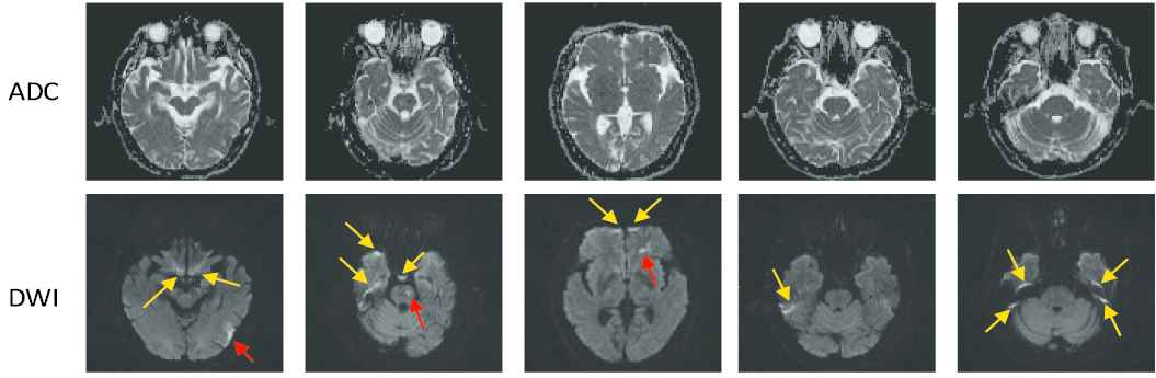
Challenge examples in acute ischemic stroke (AIS) segmentation. The first row show apparent diffusion coefficient (ADC) slices and the second row shows their corresponding diffusion-weighted image (DWI) slices. The yellow arrows identify the hyperintense due to magnetic susceptibility artifacts, and the red arrows identify the hyperintense that are true AIS lesions. Best viewed in color.
Recently, convolutional neural network-(CNN) based methods have presented tremendous ability in image classification and semantic segmentation on medical image processing [4,5]. Different from conventional image processing methods using handy-crafted image features, the CNN-based methods extract features from manually labeled data by itself. By training CNNs on a massive amount of labeled images, the CNN-based methods have achieved promising results on various organ and lesion segmentation tasks [6–9]. In order to make use of contextual information in volumetric data, in Hu et al. [10], a 3D CNN was trained to automatically localize and delineate the abdominal organs of interest with a probability prediction map, and then a time-implicit multi-phase level-set algorithm was utilized for the refinement of the multi-organ segmentation. Another 3D CNN-based method using fully convolutional DenseNet [11] was proposed for automatic segmentation of AIS [12], which achieved high performance on their test set.
Typically in a CNN, millions of parameters have to be tuned, and therefore a massive amount of images with accurate annotations are required. For instance, Sharma et al. [7] used 165 fully-labeled subjects for organ segmentation, and Zhang et al. [12] collected 152 fully-labeled subjects for lesion segmentation. Different from the images in the ImageNet [13] and COCO [14] dataset which can be easily obtained from the Internet and labeled by the ordinary people, the medical images have to be acquired by special equipment, and many well-trained clinicians are further required to precisely annotate the labels. More importantly, to perform image segmentation, most methods require pixel-by-pixel annotations to train the CNN [5,10,15–22]. For instance, in the AIS lesion segmentation task, most methods [12,23,24] required subjects with pixel-wise labels as shown in Figure 2, where each pixel was annotated as normal or lesion. Obviously, annotating the pixel-level labels are labor-intensive and time-consuming, making it even difficult to establish a large dataset. This motivates us to develop a segmentation method by using much simpler annotations. One of the simpler annotations is just annotating whether each slice incorporates lesions or not, as shown in Figure 3. Hereafter, we term this simpler annotation as weak annotation, and the data samples with weak annotations as weakly-labeled. Since the clinicians only require annotating whether each slice includes AIS lesions or not, the annotation cost can be significantly reduced, making it easier to collect a large amount of labeled data samples.
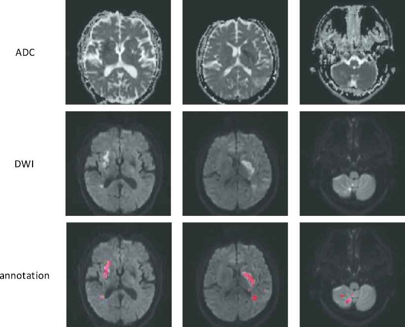
Examples of the fully-labeled subjects. The first two rows show diffusion-weighted image (ADC) slices and their corresponding diffusion-weighted image (DWI) slices. The third row shows the annotations. Best viewed in color.
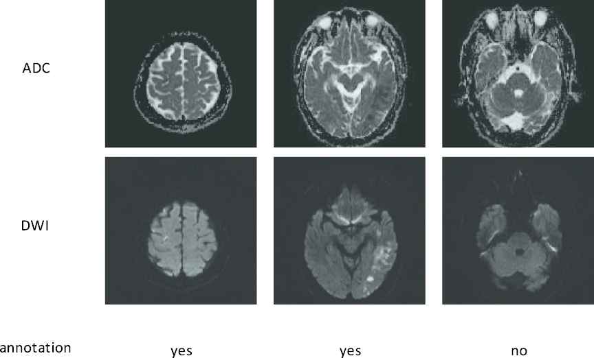
Examples of the weakly-labeled subjects. The first two rows show apparent diffusion coefficient (ADC) slices and their corresponding diffusion-weighted image (DWI) slices. The third row shows the annotations, “yes” indicates that the slice has lesion and “no” indicates the opposite.
With weakly-labeled data subjects, the CNN can generate a class activation map (CAM) for the AIS lesions [25]. The CAMs, however, were far from accurate segmentation, as they were in fact obtained from the weighted sum of low-resolution feature maps of a convolution layer. As shown in [25], despite that the lesion-wise detection rate is high, the CAMs only cover the most prominent part of the lesion. In fact, merely using weakly-supervised learning would inevitably lead to an underestimated segmentation for a large lesion, and an overestimated one for a small lesion. As we will show in this paper, by fusing multi-resolution feature maps, the proposed double-path classification network (DPC-Net) is able to output a suitable estimation for AIS lesion segmentation.
To generate a precise segmentation, we further propose to use a small amount of fully-labeled subjects to facilitate the segmentation. Despite that such semi-supervised learning methods have been adopted in image segmentation tasks by using a mixed dataset with many unlabeled samples and a few fully-labeled samples [26–28], most methods propose to adopt a self-training or co-training strategy, where the unlabeled samples were automatically annotated and added to the labeled set. Note that the generated labels will include errors, and some errors will be even strengthened during the iterative training process, leading to a risk of performing worse than a supervised approach. To solve this problem, we propose to utilize the a priori knowledge, and use the fully-labeled subjects to fine-tune a machine learning method with much fewer parameters.
In particular, we propose to use the K-means algorithm on the DWIs due to the a priori knowledge that the AIS lesions appear as hyperintense on the DWI, so that a number of candidate AIS lesion regions can be obtained. Then a region growing algorithm is adopted to combine the semantic information from the DPC-Net and the textural and spatial information from the K-means. Different from the conventional region-growing method, the algorithm adopted in this paper can automatically find an initial point from the DPC-Net rather than manually assign one. By training on 460 weakly-labeled and 5 fully-labeled subjects, the proposed method is able to achieves a mean Dice coefficient (DC) of 0.642, and a lesion-wise F1 score of 0.822 on a clinical dataset with 150 subjects.
2. RELATED WORK
There have been extensive efforts on automatic segmentation of ischemic stroke lesion recently. We roughly divided these methods into two categories, conventional methods and CNN-based methods, according to whether handy-crafted features are required. In the conventional methods, by defining some specific features on the MRIs, the ischemic stroke lesions can be identified by conventional image processing techniques or using machine-learning algorithms such as the random forest or the support vector machine (SVM). For instance, a gravitational histogram optimization-based method was proposed for ischemic stroke lesion segmentation (ISLES) using DWI [29]. To reduce the false positive (FP) rate, Mitra et al. [30] further proposed to use multimodal MRIs to extract features and identify the lesions using random forest. In Maier et al. [31], a stroke lesion segmentation method based on local features extracted from multimodal MRI, and a SVM classifier was further trained to segment the lesions. A random forest-based method was further used to identify the sub-AIS lesions [32], and achieves a top-ranking result in ISLES challenge in 2015 [33]. However, the performances of conventional methods were still not good enough as they are heavily dependent on handy-crafted features, which is understandable by the results of the recent challenge in ISLES 2015 [33].
At the same time, CNN-based methods have emerged as a powerful alternative for automatic segmentation of ischemic stroke lesion. For instance, most top-ranking methods in ISLES 2015 were based on CNNs, and the winner, DeepMedic [34], was a 3D CNN-based method, which achieved a DC of 0.59 on test set. Some other successful methods [12,18] based on CNNs in ISLES 2015 were also derived from generic CNNs architecture. Nevertheless, sub-AIS lesions have different imaging modality and lesion features from AIS lesions, so that the methods cannot be straightforwardly generalized to be used for AIS lesions. It is thus necessary to explore the methods for segmentation of AIS lesion.
Due to the lack of public dataset on the AIS lesion segmentation task, the AIS lesion segmentation methods were evaluated on institutional data were reported in the literature. A framework [23] with the combination of EDD Net and multiscale convolutional label evaluation net (MUSCLE Net) achieved a DC of 0.67 on test set by using DWIs. In order to fully utilize the MRI information, Res-Unet [24] carried out segmenting AIS lesion in multi-modality MRI. To take advantage of contextual information in volumetric data, a method based on 3D fully CNNs was proposed for AIS lesion segmentation [12], which is shown to be superior in terms of precision rate. However, these methods required hundreds of high quality fully-labeled subjects, which are very time-costly to obtain.
To reduce the burden in annotation, some semi-supervised and weakly-supervised segmentation methods were proposed. In weakly-supervised learning methods, the clinicians only need to annotate whether an image contains the target tissue or not. For instance, in Jia et al. [35] and Xu et al. [36], the cancer cells were segmented by using the labels that indicates whether a histopathology image contains cancer cells or not. When adopted in AIS segmentation, the weakly-supervised method presented high lesion-wise detection rate [25]. However, due to the lack of information on lesion positions, the CNN tends to only identify the most prominent feature that helps in classification, leading to an underestimated segmentation size when the lesion is large. For small lesions, as the segmentation results were in fact upsampled from the low-resolution feature maps in the final convolution layer, it tends to overestimate the lesion size. It implies that to accurately segment the lesions, some full annotations should be used.
The semi-supervised learning was conventionally referred to the case where the training data samples were mixed by both fully-labeled and unlabeled subjects. In medical image segmentation tasks, the network usually first learnt from the fully-labeled subjects to generate fake labels for those without full labels, and then update the network parameters based on the whole training set with both real and fake labels [26–28]. Such methods, however, risk in error propagation, as all knowledge of the target distribution came from the limited number of fully-labeled subjects.
To avoid this problem, in this paper, we propose to use a semi-supervised learning method with a few fully-labeled and many weakly-labeled subjects, where the weakly-labeled ones were used to train a CNN to extract semantic features and the fully-labeled ones were adopted to fine tune the segmentation results.
3. METHODS
In this section, we present a semi-supervised deep learning method for AIS lesion segmentation on multi-modal MR images, and the whole pipeline is presented in Figure 4. In particular, our proposed method includes two pathways. In the first pathway, we propose a DPC-Net to extract semantic information. It is able to generate probability maps (PMs) for AIS lesions with higher spatial accuracy than the CAMs in the conventional weakly-supervised learning method. In the other pathway, a K-means clustering algorithm is incorporated to obtain the lesion segmentation results, thanks to the a priori knowledge that the AIS lesions appear as hyperintense on the DWIs. Then, a region-growing algorithm is adopted to combine the results of the two pathways and generate the final segmentation result. Compared to other semi-supervised learning based methods, the proposed method does not generate any fake labels for the weakly-labeled subjects, and therefore prevent propagating the errors from a network that overfits on such a small number of fully-labeled subjects.
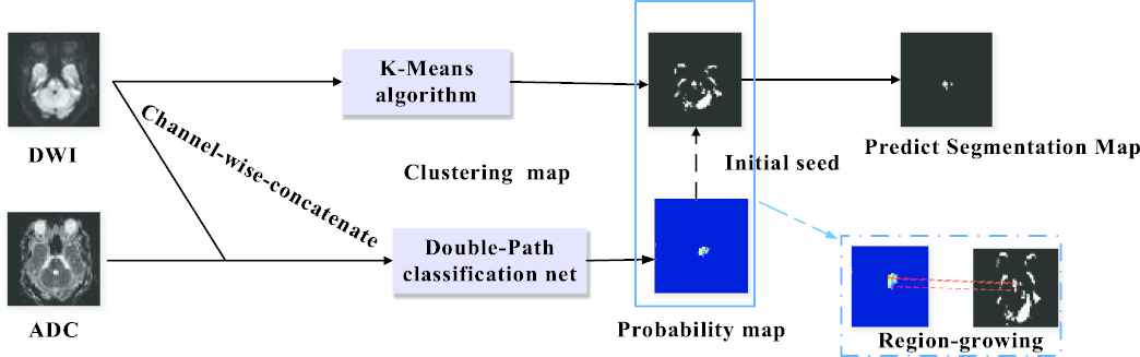
Architecture of the proposed semi-supervised learning method for lesion segmentation. Best viewed in color.
In the following subsections, we will introduce the proposed semi-supervised AIS lesion segmentation method in detail.
3.1. Double-Path Classification Network
The DPC-Net is proposed based on the VGG-16 network [37] truncated before the third maxpooling layer, and the network architecture is depicted in Figure 5(b). As we can see, we added a global average pooling (GAP) layer followed by a fully connected (FC) layer at the top of the network. Intuitively, the feature maps of the convolution block 7 is much lower than the original input images, leading to an inaccurate output PM from the view of segmentation task. To this end, we further added a side-branch with a GAP layer and a FC layer on convolution block 4 to improve the spatial resolution. As we will see in Section 4, despite that the side-branch output may contain many FPs due to the lack of semantic information, the segmentation results can be significantly improved by combining the outputs of the main branch and the side branch.
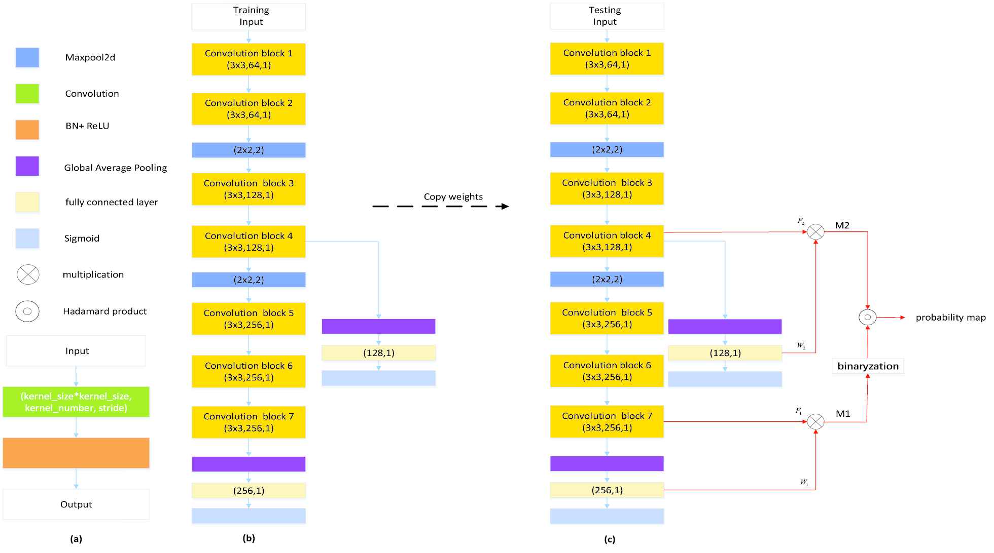
Our proposed method for generating probability maps: (a) convolution block; (b) double-path classification network; (c) inference process of the proposed double-path classification network (DPC-Net). Best viewed in color.
At the training stage, as only the slice-level label is available, a classifier is trained by using the DPC-Net shown in Figure 5(b), which can be regarded as a weakly-supervised leaning in the viewpoint of the AIS lesion segmentation. At the inference stage, as our objective is to locate the AIS lesions, the CAMs [38] is computed for both the main and the side branches to generate the segmentation seeds with adequate semantic information to highlight suspicious lesion region.
In particular, as Figure 5(c) shows, we generate the CAMs from conv-block 7 and conv-block 4, and then bilinearly upsample them to the same size as the original input, denoted as
Note that the main branch CAM output
3.2. Segmentation Map Generation
By making use of the a priori knowledge that the AIS lesions appear as hyperintense on the DWIs [3], we propose to adopt K-means algorithm and a region-growing algorithm to identify the lesion regions. In particular, the initial growing points of region-growing algorithm are given by the outputs of DPC-Net rather than manual points. Our proposed algorithm is summarized as Algorithm 1.
Algorithm 1 integrates both the pixel-level information of the original DWIs and the semantic information extracted by the DPC-Net. To achieve a better performance, the key problem is how to determine the number of clusters
Algorithm 1: Segmentation Map Generation
Input: K-Means parameter
Initialize: AIS lesion segmentation map
1: Do K-Means on the DWI and cluster the pixel into
2: Sort the
3: Preserve the group with the largest pixel values, and obtain a clustering map
4: Do connected component analysis on
5: Select a point
6: Set
7: Stop if all points that satisfy
3.3. Evaluation Metrics
In this paper, we propose to use DC, Matthews correlation coefficient (MCC) and intersection over union (IoU) to evaluate the pixel-level segmentation performance, which are defined as
Cosine similarity index (CSI) is used to measure similarity between the ground truth
In clinical diagnosis, the segmentation results on both large and small lesions are of equal importance. It is therefore necessary to use the lesion-wise metrics to evaluate the performance. In particular, we perform 3D connected component analysis on both the ground truth and the predicted segmentation. A region is said to be a TP if it appears on both ground truth and the prediction. A FP is counted if a region on the prediction has no overlapping area with any region on the ground truth; while a FN is counted if a region appears on the ground truth has no overlapping area with any region on the prediction. The mean number of TPs (m#TP), the mean number of FPs (m#FP) and the mean number of FNs (m#FN) can be then calculated by averaging over the total number of subjects.
We propose to use the lesion-wise precision rate (
4. EXPERIMENT AND RESULTS
4.1. Data and Preprocessing
The experimental data used in this study were collected from Tianjin Huanhu Hospital (Tianjin, China), which includes 615 patients with AIS lesions. All clinical images were collected from a retrospective database and anonymized prior to use. Ethical approval was granted by Tianjin Huanhu Hospital Medical Ethics Committee. MR images were acquired from three MR scanners, with two 3T MR scanners (Skyra, Siemens and Trio, Simens) and one 1.5T MR scanner (Avanto, Siemens). DWI images were acquired using a spin echo-type echo planar imaging (SE-EPI) sequence with
| MR Scanners | Skyra | Trio | Avanto |
|---|---|---|---|
| Repetition time (ms) | 5200 | 3100 | 3800 |
| Echo time (ms) | 80 | 99 | 102 |
| Flip angle (o) | 150 | 120 | 150 |
| Number of excitations | 1 | 1 | 3 |
| Field of view (mm2) | 240 × 240 | 200 × 200 | 240 × 240 |
| Matrix size | 130 × 130 | 132 × 132 | 192 × 192 |
| Slice thickness (mm) | 5 | 6 | 5 |
| Slice spacing (mm) | 1.5 | 1.8 | 1.5 |
| Number of slices | 21 | 17 | 21 |
Parameters used in diffusion-weighted image (DWI) acquisition.
The ischemic lesions were manually annotated by two experienced experts (Dr. Song Jin and Dr. Chen Cao) from Tianjin Huanhu Hospital.
We split the whole dataset into two subsets: training set and test set. The training set includes 460 subjects with weak labels for training and validating the DPC-Net, and 5 subjects with precise pixel-level labels to fine-tune clustering number
As the MR images were acquired on the three different MR scanners, the matrix size varies. Therefore, we resample all the MR images to the same size of 192
4.2. Setup and Implementation
The hyperparameters of the proposed DPC-Net are shown in Figure 5. We initialize these networks by Xavier’s method [39] and use the Adam method [40] with
The experiments are performed on a computer with an Intel Core i7-6800K CPU, 64GB RAM and Nvidia GeForce 1080Ti GPU with 11GB memory. The computer operates on Windows 10 with CUDA 9.0. The network is implemented in PyTorch 0.4 (
4.3. Results
In our experiment, 460 weakly-labeled subjects and 5 fully-labeled subjects are used to train and fine-tune the parameters. The 5 fully-labeled subjects are abbreviated as fine-tuning set. Figure 6 presents the segmentation results of our proposed method. The CAM results obtained from a naïve VGG-16 based CAM method [38], denoted as CAM-baseline, and the output PM of our proposed DPC-Net, denoted as PM-DPC-Net, are also presented for comparison. As shown in Figure 6, the CAM-based methods can successfully identify and localize the AIS lesions. Despite that the magnetic artifacts have similar appearances as the AIS lesions on the DWIs, the deep-learning-based methods can distinguish the lesions from the artifacts thanks to the semantic information extracted from the weakly-labeled subjects. From the aspect of segmentation, however, the CAM-baseline tends to segment much larger area than the actual AIS lesion, due to the fact that the output PMs in conventional CAM method is obtained from features maps with much lower resolution than the original images. Our proposed DPC-Net significantly reduces the areas of the suspicious regions thanks to the side branch output, but underestimates the lesion areas in some cases. By integrating both pixel-level clustering and the PM-DPC-Net output, the proposed method is sensitive to both large and small lesions, and presents much better segmentation results over the CAM-baseline and PM-DPC-Net.
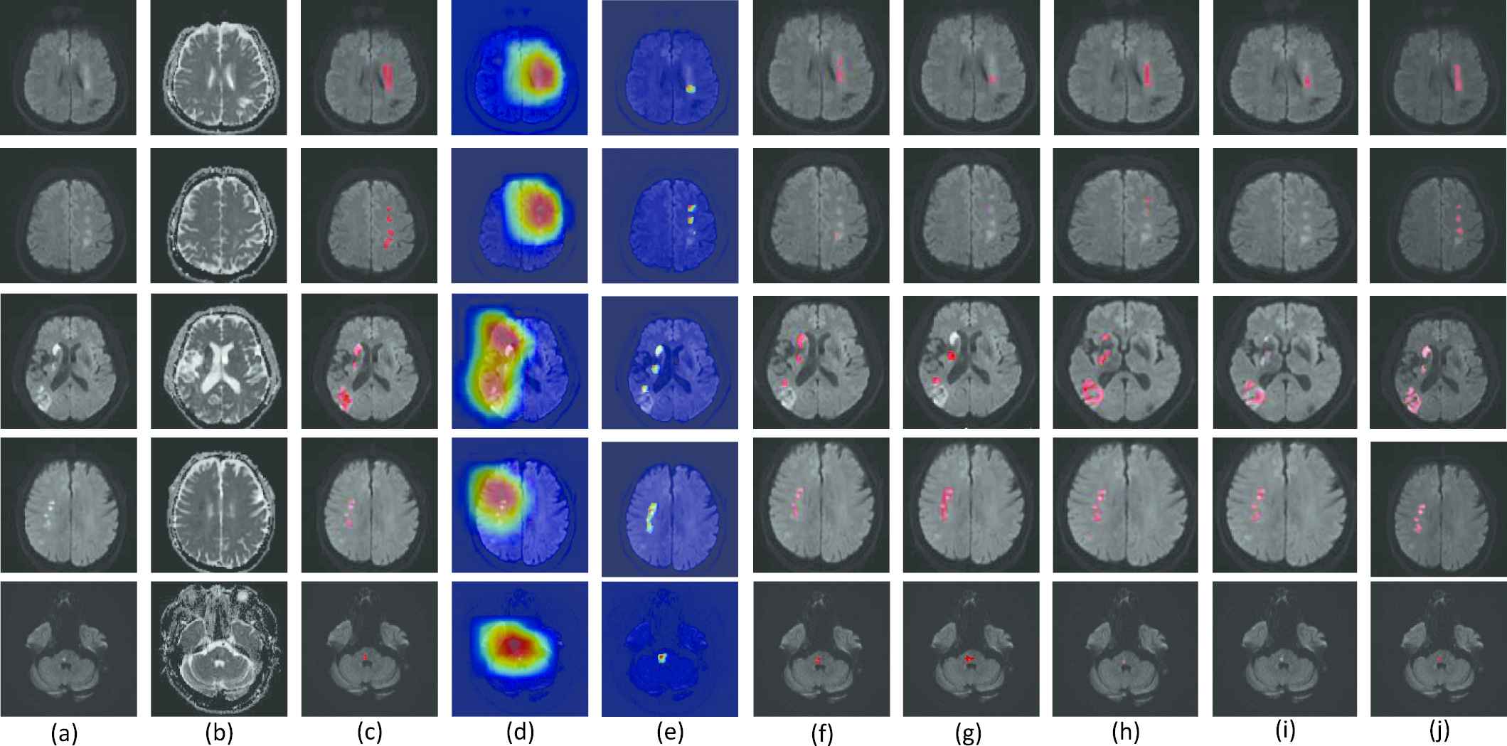
Examples of lesion segmentation, class activation maps (CAMs) and probability maps (PMs). (a-c) are the original diffusion-weighted image (DWI), apparent diffusion coefficient (ADC) map and ground truth, respectively. (d-j) are the CAMs of the baseline VGG-16 Network (CAM-baseline [38]), the PMs of double-path classification network (DPC-Net) (PM-DPC-Net), the segmentation results of U-net [41], FCN-8s [19], Res-Unet [24], the method proposed in [42] and our proposed method. The CAMs and PMs are depicted on the DWI, and the redder with the color map, the more likely it is to represent the lesion region. The segmentations are also depicted on the DWI, and highlighted in red. Best viewed in color.
For the sake of comparison with other methods of semantic segmentation, we also train and evaluate a U-net [41], a FCN-8s [19], a Res-Unet [24] and the method proposed in [42] on our dataset. The encoder parts of these methods are also pretrained as a classifier on our weakly-labeled data for fairness, then these methods are retrained on the 5 fully-labeled data. As the Figure 6 shows, the U-net, FCN-8s, Res-Unet and the proposed in [42] overlook some lesions in segmentation process, as merely training on 5 subjects are far from adequate to train a CNN with so much parameters. Besides, FCN-8s uses three-scale feature fusion and the outputs of its last convolutional layer resampled to the size of input image require interpolation of 32 times, which will overestimate some lesion regions.
The numerical evaluation results on the test set with 150 fully-labeled subjects are summarized in Table 2. For CAM-baseline and PM-DPC-Net, the thresholds to generate the binary segmentation are selected by using the fine-tuning set. For our proposed method, these fully-labeled images are used to tune both the threshold
| Method | (δ,K) | DC | PL | RL | F1 | CSI | MCC | mIoU |
|---|---|---|---|---|---|---|---|---|
| CAM-baseline [38] | (0.7, *) | 0.091 | 0.854 | 0.791 | 0.821 | 0.169 | 0.169 | 0.050 |
| U-net [41] | (*, *) | 0.582 | 0.791 | 0.670 | 0.726 | 0.639 | 0.639 | 0.448 |
| FCN-8s [19] | (*, * ) | 0.405 | 0.953 | 0.622 | 0.753 | 0.498 | 0.498 | 0.281 |
| Res-Unet [24] | (*, * ) | 0.535 | 0.438 | 0.840 | 0.576 | 0.567 | 0.567 | 0.395 |
| Few-shot [42] | (*, * ) | 0.269 | 0.115 | 0.551 | 0.191 | 0.295 | 0.295 | 0.179 |
| PM-DPC-Net | (0.3, *) | 0.475 | 0.790 | 0.742 | 0.765 | 0.522 | 0.522 | 0.325 |
| Ours | (0.41,6) | 0.642 | 0.880 | 0.772 | 0.822 | 0.680 | 0.680 | 0.512 |
* indicates that the method does not have this parameter
The best results are highlighted in bold.
CAM, class activation map; DPC-Net, double-path classification network; DC, Dice coefficient; MCC, Matthews correlation coefficient; CSI, Cosine similarity index.
The evaluation measurements on test set.
From the aspect of the pixel-level metrics, our proposed method achieves a mean DC of 0.642, a mean CSI of 0.680, a mean MCC of 0.680 and a mean IoU (mIoU) of 0.512, which are higher than the results obtained by the competitors. In fact, such performance is very close to the method trained on fully-labeled images [23]. From the aspect of lesion-wise metrics, our proposed method achieves the precision rate of 0.880, which is higher than other methods except for FCN-8s. In fact, FCN-8s has 19 missed diagnosis subjects while our method only has 2 missed diagnosis, which leads the less FPs of FCN-8s. The recall rate, however, is worse than the Res-Unet due to the fact that the Res-Unet has the residual unit which can promote gradient propagation so as to reduce the FNs. The K-means clustering algorithm may also fail to group all lesions to the same group if the intensities of different lesions differ significantly from each other.
Figure 7 further plots the scatter map between the volumes of the ground truth and the predicted segmentation, where the purple line indicates a perfect match between the predicted volumes and the ground truth volumes. As the Figure 7 shows, the predicted volumes of our proposed method are closer to the true volumes than the competitors.
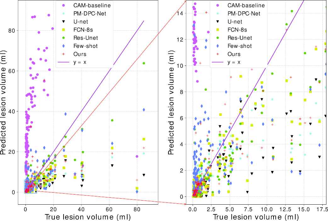
Predicted lesion volume versus the ground truth volume.
5. DISCUSSIONS
5.1. Effect of Clustering Numbers
As the AIS lesions appear as hyperintense on the DWI, we adopt K-means clustering algorithm to identify the hyperintensive regions. Note that the artifacts on the DWIs are also the hyperintensive regions, making it crucial to fine-tune the value of
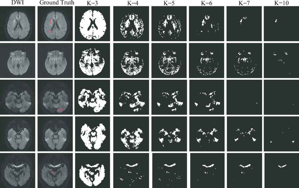
Examples of clustering map. The first two columns show the original diffusion-weighted image (DWI) and the ground truth, respectively. The last six columns show the clustering maps with the clustering number of 3, 4, 5, 6, 7 and 10, respectively. The ground truth is depicted on the DWI, and highlighted in red. Best viewed in color.
In our work, we propose to use a small amount of fully-labeled subjects to search the optimal parameters in a grid search manner, and use DC as the metric. The results with
| (δ, K) | (0.8, 3) | (0.7, 4) | (0.6, 5) | (0.4, 6) | (0.3, 7) | (0.1, 10) | ||||||
|---|---|---|---|---|---|---|---|---|---|---|---|---|
| Data Set | FT-Set | Test Set | FT-Set | Test Set | FT-Set | Test Set | FT-Set | Test Set | FT-Set | Test Set | FT-Set | Test Set |
| DC | 0.069 | 0.089 | 0.198 | 0.322 | 0.411 | 0.594 | 0.556 | 0.642 | 0.366 | 0.610 | 0.296 | 0.473 |
| PL | 0.875 | 0.980 | 0.857 | 0.951 | 0.750 | 0.919 | 0.778 | 0.880 | 0.778 | 0.890 | 0.667 | 0.916 |
| RL | 0.875 | 0.823 | 0.750 | 0.789 | 0.750 | 0.769 | 0.875 | 0.772 | 0.875 | 0.741 | 0.500 | 0.667 |
| F1 | 0.875 | 0.895 | 0.800 | 0.862 | 0.750 | 0.837 | 0.824 | 0.822 | 0.824 | 0.809 | 0.571 | 0.772 |
| CSI | 0.164 | 0.166 | 0.265 | 0.394 | 0.449 | 0.634 | 0.571 | 0.680 | 0.425 | 0.664 | 0.349 | 0.564 |
| MCC | 0.163 | 0.164 | 0.264 | 0.393 | 0.449 | 0.634 | 0.571 | 0.679 | 0.425 | 0.663 | 0.349 | 0.564 |
| mIoU | 0.037 | 0.057 | 0.119 | 0.232 | 0.281 | 0.470 | 0.424 | 0.512 | 0.254 | 0.481 | 0.202 | 0.351 |
Evaluation results under the variety of
5.2. Impact of Lesion Size
As pointed out in [45], a AIS lesion is classified as a lacunar infarction (LI) lesion if its diameter is smaller than 1.5 cm. Clinically, the LI stroke accounts for 85% of all AIS patients. However, it is much difficult to be diagnosed in clinical practice, especially when it is too small to be noticed. It is, therefore, very necessary to evaluate the performance on subjects with small lesions.
In this subsection, we further divide our test set to a large lesion set and a small lesion set. A subject is categorized into the small lesion set only if all of the lesions are LI lesions. Otherwise, it will be included in the large lesion set. In our test set, the large lesion and the small lesion sets include 60 subjects and 90 subjects respectively. As Table 4 shows, our proposed method achieves a DC of 0.708 on the small lesion set, while a DC of 0.543 on the large lesion set. Meanwhile, the
| Data Set | DC | PL | RL | F1 | CSI | MCC | mIoU |
|---|---|---|---|---|---|---|---|
| Test set | 0.642 | 0.880 | 0.772 | 0.822 | 0.680 | 0.680 | 0.512 |
| Large lesions set | 0.543 | 0.889 | 0.705 | 0.786 | 0.583 | 0.582 | 0.397 |
| Small lesions set | 0.708 | 0.867 | 0.901 | 0.883 | 0.746 | 0.746 | 0.588 |
CSI, Cosine similarity index; MCC, Matthews correlation coefficient.
The best results are highlighted in bold.
Evaluation results on test set, large lesions set and small lesions set, respectively. The best results are highlighted in bold.
In clinical diagnosis, large lesions are more easily diagnosed, while small lesions are not. Our proposed method achieves high performance on small lesions, which might be of a good inspiration for other methods.
5.3. Discussions of the DPC-Net
In Section 3.1, we propose the DPC-Net to generate the PMs. The DPC-Net consists of two branches that are based on the convolutional block 4 and convolutional block 7 of the VGG-16. In this section, we combine different convolutional block of VGG-16 to generate many new DPC-Nets for comparison. In particular, we only focus on the convolutional blocks next to the maxpooling layer for reason that they extract the largest semantic information at the current feature map scale. Meanwhile, as a shallow convolution layer, the convolutional block 2 cannot extract semantic information well. Hence the combination of the new DPC-Nets includes convolutional block (4, 10), convolutional block (7, 10), convolutional block (4, 13), convolutional block (7, 13) and convolutional block (10, 13), which are referred to as the “variants” for simplicity. The Figure 9 plots the PMs generated by the “variants” and our proposed DPC-Net. We propose to use convolutional block 4 and convolutional block 7 to generate the PMs for reason that the feature maps of convolutional block 7 are much higher spatial resolution than that of deeper convolutional blocks, which can remain the approximate suspicious lesion regions to the true lesion regions when its feature maps are interpolated into the original input size. Besides, the convolutional block 4 is the closest to the convolutional block 7, which can help each other to extract semantic information well. In contrast, the “variants” use deeper convolutional blocks to generate PMs. Their feature maps have lower spatial resolution that would lead to larger suspicious lesion regions than the true lesion regions when their feature maps are interpolated into the original input size, which further provide larger growing seed points for the cluster map on the DWI so that the segmented lesions are larger than the true lesions. Table 5 summarizes the evaluation results under the “variants” and our proposed DPC-Net. As we can see, the proposed combination strategy achieves the best results in terms of both lesion-wise metrics
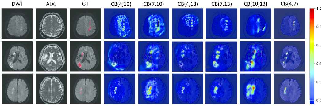
Examples of probability maps (PMs). The PMs are depicted on the diffusion-weighted image (DWI), and the redder with the color map, the more likely it is to represent the lesion region. The convolutional block is abbreviated to CB for simplicity. CB (4, 7) denotes our proposed double-path classification network (DPC-Net). Best viewed in color.
| Variants | DC | PL | RL | F1 | CSI | MCC | mIoU |
|---|---|---|---|---|---|---|---|
| CB (4, 10) | 0.626 | 0.852 | 0.707 | 0.773 | 0.661 | 0.661 | 0.498 |
| CB (7, 10) | 0.541 | 0.486 | 0.690 | 0.570 | 0.582 | 0.582 | 0.412 |
| CB (4, 13) | 0.602 | 0.810 | 0.697 | 0.750 | 0.643 | 0.643 | 0.475 |
| CB (7, 13) | 0.628 | 0.772 | 0.748 | 0.760 | 0.663 | 0.662 | 0.497 |
| CB (10, 13) | 0.317 | 0.127 | 0.660 | 0.213 | 0.379 | 0.379 | 0.210 |
| CB (4, 7) | 0.642 | 0.880 | 0.772 | 0.822 | 0.680 | 0.680 | 0.512 |
The convolutional block is abbreviated to CB for simplicity. CB (4, 7) denotes our proposed DPC-Net.
DPC-Net, double-path classification network; DC, Dice coefficient; MCC, Matthews correlation coefficient; CSI, Cosine similarity index.
Evaluation results under the “variants” and our proposed DPC-Net. The convolutional block is abbreviated to CB for simplicity. CB (4, 7) denotes our proposed DPC-Net.
6. CONCLUSION
In this paper, we present a semi-supervised method for AIS lesion segmentation, where 460 weakly-labeled subjects are used to train the DPC-Net and then 5 fully-labeled subjects are used to fine-tune the parameters in a supervised way. The proposed semi-supervised method presents a high segmentation accuracy on the clinical MR images with a DC of 0.642. More importantly, it presents very high precision of 0.880, which is of paramount importance in avoiding misdiagnosis in clinical scenario. Meanwhile, the proposed method largely reduces the expense of obtaining a large number of fully-labeled subjects in a supervised setting, which is more meaningful in terms of engineering maneuverability.
In fact, lesion segmentation using unsupervised learning is an interesting topic to study, and has attracted the attentions among researchers [46]. However, the magnetic artifacts have similar appearances as the AIS lesions on the DWIs and it is difficult to distinguish the AIS lesions from the artifacts in a fully-unsupervised manner. In K-means, for instance, as we have shown in Figure 8, the unsupervised learning method cannot extract the necessary semantic information for segmentation, leading to many FPs. Such results indicate that to detect the abnormality in an unsupervised way, the methods should be designed more carefully. We would very much like to investigate the unsupervised learning methods for AIS segmentation in our future work.
CONFLICTS OF INTEREST
All authors of this manuscript do not have financial and personal relationships with other people or organizations that could inappropriately influence their work.
AUTHORS' CONTRIBUTIONS
Bin Zhao: Conceptualization, Methodology, Software, Writing; Shuxue Ding: Project Administration, Resources, Investigation; Hong Wu and Guohua Liu: Reviewing and Editing; Chen Cao and Song Jin: Data Curation, Visualization, Validation; Zhiyang Liu: Supervision, Validation and Investigation.
ACKNOWLEDGMENTS
This work is supported in part by the National Natural Science Foundation of China [grant numbers 61871239, 62076077] and the Natural Science Foundation of Tianjin (20JCQNJC0125).
REFERENCES
Cite this article
TY  - JOUR
AU  - Bin Zhao
AU  - Shuxue Ding
AU  - Hong Wu
AU  - Guohua Liu
AU  - Chen Cao
AU  - Song Jin
AU  - Zhiyang Liu
PY  - 2021
DA  - 2021/02/10
TI  - Automatic Acute Ischemic Stroke Lesion Segmentation Using Semi-supervised Learning
JO  - International Journal of Computational Intelligence Systems
SP  - 723
EP  - 733
VL  - 14
IS  - 1
SN  - 1875-6883
UR  - https://doi.org/10.2991/ijcis.d.210205.001
DO  - 10.2991/ijcis.d.210205.001
ID  - Zhao2021
ER  -