
The Red Colobuses Monkey: A New Nature–Inspired Metaheuristic Optimization Algorithm
 , Maha Mahmood1, Dac-Nhuong Le3, 4, *,
 - DOI
- 10.2991/ijcis.d.210301.004How to use a DOI?
- Keywords
- Red colobuses monkey; Optimization; Metaheuristic; Particle swarm optimization
- Abstract
The presented study suggests a new nature–inspired metaheuristic optimization algorithm referred to as Red Colobuses Monkey (RCM) that can be used for optimization problems; this algorithm mimics the behavior related to red monkeys in nature. In preparation for proving the suggested algorithm's advantages, a set of standard unconstrained and constrained test functions is employed, sixty–four of identified test functions utilized in optimization were applied as benchmarks for checking the RCM performance. The solutions have also been upgrading their positions based on the optimal solution, which was reached thus far. Also, RCM can replace the worst red monkey by the best child found so far to give an extra enhancement to the solutions. Also, comparative performance checks with Biogeography–Based Optimizer (BBO), Artificial–Bee–Colony (ABC), Particle Swarm Optimization (PSO), and Gravitational Search Algorithm (GSA) were done. The acquired results showed that RCM is competitive in comparison to the chosen metaheuristic algorithms.
- Copyright
- © 2021 The Authors. Published by Atlantis Press B.V.
- Open Access
- This is an open access article distributed under the CC BY-NC 4.0 license (http://creativecommons.org/licenses/by-nc/4.0/).
1. INTRODUCTION
Optimization utilizing metaheuristics is of high importance; for instance, Particle Swarm Optimization (PSO) [1], Genetic Algorithm (GA) [2], and Ant Colony Optimization (ACO) [3]. Also, along with the various theoretical researches, there were various applications to optimization methods in many fields. Four significant reasons were explaining such matters: derivation free mechanism, simplicity, flexibility, and local optima avoidance. Generally, there were based on fundamental notions [4]. The stochastic optimization (metaheuristic) algorithms belong to a family in which their algorithms have stochastic operations involving evolutionary algorithms; yet, randomness is the main character or such algorithm. PSO [5] seeks inputs for finding the optimum ones with the best fitness value over the iteration course for enhancing the rest of the solutions. Due to the high–flexibility, gradient–free technique, and low probability of local optima stagnation, applications utilized various meta–heuristics in many industry and science areas [6]. The swarm–based approaches are mimicking the social behavior regarding groups of animals. PSO is the primary algorithm initially introduced via Eberhart and Kennedy [7]; such an algorithm was inspired by the bird flocking's social behavior. The algorithm applies some particles (candidate solutions) flying around in search space for finding the best solution (for instance, optimal position). In the meantime, they are all tracking the best location (best solution) in their paths. Put differently; particles consider their best solutions and the best solution obtained so far by the swarm.
This paper provides a study regarding the development of an optimization algorithm utilizing primary mathematical function in the metaheuristic field, the resulted algorithm called Red Colobuses Monkey (RCM). This algorithm has a few parameters that make it easy to implement. The proposed algorithm can also balance between exploitation and exploration stages that suit various optimization problems. The rest of this study is provided in the following way: Section 2 shows the relevant works. Section 3 presents the inspiration of the RCM Algorithm. Section 4 shows the mathematical model and the algorithm of RCM. Section 5 presents the discussion and results of the test functions. Section 6 presents the main conclusions of the paper. Finally, we suggest several future research directions.
2. LITERATURE REVIEW
Single solutions based and population–based are the two main types of stochastic optimization techniques. The single based class of algorithms operates the optimization process with a single random solution and improves it over a predefined number of generations. Also, the population–based can either work together or compete against each other. Three population–based algorithms are based on inspiration: Swarm inspired, evolution inspired, and physics–inspired algorithms [7]. The swarm–based algorithms are majorly mimicking the individual and social behavior regarding herds, swarms, schools, or groups of creatures in nature. One of the most known algorithms inspired by the birds' behavior is the PSO algorithm [8]. This algorithm mimics the collective behavior of birds in the population faces sudden changes. There are some other swarms and nature–inspired algorithms; those are Firefly Algorithm (FA) that is used effectively in various domains of optimization problems. The process of identifying the optimal solution while keeping something as useful and functional as possible, by reducing or adding the problem's parameters when needed, called the Optimization process. Several optimization problems are addressed by inspiring fireflies' behavior; those problems are multiobjective, chaotic, discrete, and many more. It was found that researchers that are solved the optimization problems in the computer science and engineering domain mostly applied FA. Some of them are improved or hybridized with other techniques for obtaining better performance [9].
Crow Swarm Optimization (CSO) can be defined as one of the novel metaheuristic optimization techniques proposed to solve the multidepot multiple traveling salesmen problem (MMTSP). CSO is derived from the behavior of American Crow in finding the shortest path while searching for food. In solving the MMTSP, the algorithm is observed with randomly chosen cities as depots, then visiting as much as a possible number of cities by a salesman. The implementation is observed with several datasets from Traveling Salesman Problem Library (TSPLIB) [10].
Meerkat Swarm Optimization (MSO) algorithm is used for solving Multiple Traveling Salesman Problem and guarantee good quality solution in a reasonable time for real–life problems. MSO is one of the metaheuristic optimization algorithms developed from the meerkat's behavior in finding the shortest path. MSO is a new intelligent method proposed for examining timetabling problems inspired by meerkat swarm's behavior in nature. The MSO algorithm simulates cooperative behavior such as caring and foraging of meerkats. Meerkats in the MSO algorithm has its leader (called alpha), and they divided into two subgroups, one for foraging while the other stays as a babysitter for pups in burrows [11].
Blue Monkey (BM) algorithm is defined as one of the novel metaheuristic algorithms inspired by blue monkeys' behavior in nature, while such an approach identifies the number of males in a single group. Typically, blue monkey groups have just a single adult male than the other forest guenons [12]. Majorly, Evolutionary Algorithms (EAs) were equipped with recombination and selection operators for exploring the search spaces.
This work aims to study the effect of the suggested transfer functions in the RCM for observing their efficiency when used to various heuristic algorithms. PSO is operating to enhance the vector, whereas GA was utilized to modify the decision vectors using genetic operators. The balance between exploitation and exploration capabilities was further enhanced by incorporating genetic operators, mutation, and crossover in PSO. Also, the problem's constraints were managed by using a parameter–free penalty function [13]. Intuitionistic fuzzy set (IFS) through using uncertain, imprecise, and vague data. In the literature, the IFS membership functions were evaluated using fuzzy arithmetic operations in collected data and therefore contain many uncertainties. So, there is a need to optimize such spread by formulating nonlinear optimization problems via ordinary arithmetic operations rather than fuzzy operations. PSO was utilized to construct their membership functions [14–30].
From all the above, it can be seen that no one metaheuristics algorithm can solve all kinds of problem domains; therefore, there is always a need for new algorithms that can address many types of problem domains.
3. THE INSPIRATION OF THE RED COLOBUSES MONKEY
In the Gambia and other West African forests, the Western Red Colobus Monkeys, also referred to as bay colobus, were found. These herbivores' main characters are leaves eaters and tend to gather in groups of 20–80 individuals, even though they are splitting into small groups in foraging. Leopards were from the natural predators' groups develop a hierarchy of dominance specified via aggressive behavior. Initially, food, grooming, and sexual partners were distributed among high–ranking individuals and succeeded via low-ranking individuals [13]. The majority of these monkeys live in large troops of 80 individuals, whereas the average number might be approximately (20–40). Those groups tend to have more females at a 2:1 ratio compared to males.
In some families of these monkeys' troops, the male monkeys usually choose to stay close to the original groups. However, the female monkeys, on the other hand, tend to move together in smaller numbers. Red colobus monkeys have mixed with other troops. The results of such interactions are either violent or passive; one troop is trying to control the rest. Remarkable behaviors appear when red turn to be angry and restless and somewhat nomadic [14], such state was reached in the case when young monkeys are deserting their natal troops and attempt to join another group, this is not merely because of the suspicion of some troops to any new guest, and they turn to be violent when new monkeys attempt to join. The diet–related to red colobus monkeys majorly includes flowers, young leaves, and unripe fruits, while the red–tailed monkeys were active in the evening and early morning, which was specified as a diurnal activity. Charcoal or clay could also be a food choice for them for helping with cyanide combating that a few leaves could contain. A mother could transfer the medicinal sure of the plans they eat to their children. Therefore, some appear to have better digestion for the toxic plans than the other primates [15]. The red colobus monkeys were majorly suitable to their vegetarian and changed diet tendency for wasting time in the forest's habitats, which has been associated with the presence of fruit resources and structural characteristics such as large fruit patches [16]. One male and females, along with their offspring, are usually the ones dominant for each group. Generally, these groups choose to stay close for a long period, except for the male who reaches maturity. Such a habit is teaching babies for reacting with all the monkeys in later years.
4. THE ALGORITHM AND THE MATHEMATICAL MODEL
This section is providing the RCM algorithm as well as its mathematical model.
4.1. Group Division
RCM algorithmic program is mimicking the red monkey's behavior. For modeling, these interactions, each of the clusters in the monkey area unit required maneuvering over the search area. As it has been indicated previously, in the case where they have been divided to teams, every team of monkeys will have one male, and no necessary the male is the leader, but the choice of leader depended on body and combat power, who will be looking for food places at the areas of long distance, while the stronger monkey is not within the scope of the conventional vision. Also, there are not many interactions between male Cercopithecus mitis and young ones. Young males must go out quickly due to the territorial aspect associated with Cercopithecus mitis to be more successful, as they are entering challenges with dominant males from other families. If they can defeat that male, they will be leaders in the family and offer places to live, food supplies, and socialization for the young males.
4.2. Position Update
The position update regarding every one of the red monkeys in a group is based on the position of the best red monkey of the group; such behavior was delineating through the following formulas:
PB represents the monkey body power (a random number between
PA represents the monkey combat power (a randomly chosen number between
X represents the position of the red monkey;
To update the position related to the children of red monkey, the next equations have been utilized:
PBch represents the power rate of the child body;
PAch is representing the child combat power rate;
Xch represent the position of the child;
“rand” represents a random number in the range of
The major steps of RCM might be summarized as the pseudo–code indicated in the Algorithm 1.
It is worth mentioning that all parameters of RCM can be set either by experiments or depending on the problem's nature, which must be solved. RCM is characterized by a few parameters that make it easy to implement; RCM can also balance between exploitation and exploration phases, making it suitable to solve many optimization problems.
5. RESULTS AND DISCUSSION
Concerning the presented section, the RCM will be tested and estimated utilizing 64–benchmark functions, a few of the functions, the first 23 referred to as unimodal, traditional, and simple ones. In contrast, the others are referred to as multimodal (not fixed and fixed), which are utilized via various research; the functions were selected for testing RCM performance and comparing the results of this work with other standard metaheuristic results algorithms. Also, the chosen 64–test functions will be displayed in Tables 1–3 in which D represents the function dimensions, range represents the limits of the search space related to the function, whereas Opt represents optimum value.
| Equation | Test Name | D | Range | Opt |
|---|---|---|---|---|
| Sphere | 30 | 100, –100 | 0 | |
| Schwefel 2.22 | 2 | 100, −100 | 0 | |
| Schwefel 2.21 | 2 | 100, −100 | 0 | |
| Schwefel 1.2 | 2 | 100, −100 | 0 | |
| Ackley 2 | 2 | 32, −32 | −200 | |
| Bohachevskyn N.1 | 2 | 100, −100 | 0 | |
| Booth | 2 | 10, −10 | 0 | |
| Zakharov | 2 | 5.12, −5.12 | 0 | |
| Dixon–Price | 2 | 10, −10 | 0 | |
| Exponential | 30 | 1, −1 | −1 | |
| Matyas | 2 | 10, −10 | 0 | |
| Schwefel 2.23 | 2 | 100, −100 | 0 | |
| Schwefel 2.20 | 2 | 100, −100 | 0 | |
| Schaffer N2 | 2 | 36, −36 | 0 | |
| Schaffer N3 | 2 | 100, −100 | 0.00156 | |
| Schaffer N1 | 2 | 100, −100 | 0 | |
| Powell | 10 | 5, −4 | 0 | |
| Power Sum | 4 | 4, 0 | 0 | |
| Drop wave | 2 | −5.12, 5.12 | −1 | |
| Langermann | 2 | −1, 4 | −2.1950 | |
| Brent | 2 | −20, 0 | ||
| Leon | 2 | 0, 10 | 0 | |
| Sum Squares | 10 | −10, 10 | 0 |
Unimodal benchmark functions.
| Equation | Test Name | Type | D | Range | Opt |
|---|---|---|---|---|---|
| Ackley | N | 2 | 10, −10 | 0 | |
| Step 1 | N | 30 | 100, −100 | 0 | |
| Quartic | N | 10 | 1.28, –1.28 | 0 | |
| Six–Hump Camel | N | 2 | 5, −5 | −1.0316 | |
| Goldstein Price | N | 2 | 2, −2 | 3 | |
| Schwefel 2.26 | N | 30 | 500, −500 | −12569.5 | |
| Penalized 1 | N | 2 | 50, −50 | 0 | |
| Penalized 2 | N | 2 | 50, −50 | 0 | |
| Three–Hump Camel | N | 2 | 5, −5 | 0 | |
| Bohachevskyn N.2 | N | 2 | 10, −10 | 0 | |
| Brid | N | 2 | −106.7645 | ||
| Cross in Tiny | N | 2 | 10, −10 | −2.06261 | |
| Keane | N | 2 | 10, 0 | −0.6737 | |
| Egg Holder | N | 2 | 512, −512 | −959.641 | |
| Holder | N | 2 | 10, −10 | −19.2085 | |
| Schwefel | N | 2 | 500, −500 | 0 | |
| Michalewics | N | 2 | 2.21, 1.57 | −1.8013 | |
| Periodic | N | 30 | −10, 10 | 0.9 | |
| Qing | N | 10 | −500, 500 | 0 | |
| Salomon | N | 10 | −100, 100 | 0 | |
| xinsheyangn2fcn | N | 10 | 0 | ||
| Xin–She Yang N. 4 | N | 10 | −10, 10 | −1 | |
| Brown | N | 10 | −1, 4 | 0 |
Multimodal benchmark functions (not fixed).
| Equation | Test Name | Type | D | Range | Opt |
|---|---|---|---|---|---|
| Branin | F | 2 | 15, −5 | 0.3979 | |
| Hartmann 6–D | F | 3 | 1, 0 | −3.8628 | |
| Hartmann 6–D | F | 6 | 1, 0 | −3.3224 | |
| Ackley 3 | F | 2 | 32, −32 | −195.629 | |
| Easom | F | 2 | 100, −100 | −1 | |
| Trid | F | 6 | 36, 36 | −50 | |
| Gramacy & Lee | F | 1 | 2.5, 0.5 | −0.869 | |
| Alpine N. 1 | F | 2 | −1, 2 | 0 | |
| Alpine N.2 | F | 2 | 0, 10 | 2.2808n | |
| Bartels Conn | F | 2 | −500, 500 | 1 | |
| Beale | F | 2 | −4.5, 4.5 | 0 | |
| Bukin N. 6 | F | 2 | −3, 3 | 0 | |
| Deckkers–Aarts | F | 2 | −20, 20 | −24771.09375 | |
| Egg Crate | F | 2 | −5, 5 | 0 | |
| Himmelblau | F | 2 | −6, 6 | 0 | |
| Levi N. 13 | F | 2 | −10, 10 | 0 | |
| McCormick | F | 2 | −1.5, 4 | −1.9133 | |
| wolfefcn | F | 3 | 0, 2 | 0 |
Multimodal benchmark functions (fixed).
Generally, the used test functions were minimization functions that have been multimodal or unimodal benchmark functions (not fixed and fixed).
The proposed RCM is carried out thirty times for each benchmark function, while the statistical results (average as well as standard deviation) regarding the comparison of RCM with Artificial–Bee–Colony (ABC) [17], PSO [18], Gravitational Search Algorithm (GSA) [19], Grey Wolf Optimizer (GWO) [20] and Biogeography–Based Optimizer (BBO) [21] are provided in Table 3 for unimodal functions as well as in Table 4 for multimodal functions
| RCM |
ABC |
PSO |
||||
|---|---|---|---|---|---|---|
| Function | Average | Std | Average | Std | Average | Std |
| F1 | 9.04E–13 | 1.32E–12 | 0.001253 | 0.0008112 | 2.54E–08 | 7.98E–08 |
| F2 | 6.69E–47 | 0 | 0.0002537 | 0.0001524 | 1.05E–55 | 5.15E–55 |
| F3 | 3.61E–47 | 0 | 0.0016628 | 0.0010982 | 2.03E–51 | 1.10E–50 |
| F4 | 9.12E–91 | 0 | 4.55E–06 | 6.63E–06 | 1.86E–90 | 1.02E–89 |
| F5 | −200 | 0 | −199.9998 | 0.0001017 | −200 | 0 |
| F6 | 0 | 0 | 1.42E–05 | 1.41E–05 | 1.67E–16 | 5.89E–16 |
| F7 | 0 | 0 | 4.52E–07 | 5.79E–07 | 6.97E–30 | 2.48E–29 |
| F8 | 9.86E–95 | 0 | 1.84E–09 | 1.70E–09 | 4.08E–104 | 2.08E–103 |
| F9 | 3.70E–32 | 5.67E–48 | 2.20E–06 | 2.14E–06 | 0.0852267 | 0.4084247 |
| F10 | −1 | 0 | −0.999941 | 3.82E–05 | −1 | 0 |
| F11 | 1.00E–89 | 0 | 1.33E–07 | 1.36E–07 | 6.77E–66 | 3.71E–65 |
| F12 | 0 | 0 | 2.95E–31 | 9.24E–31 | 0 | 0 |
| F13 | 1.11E–45 | 0 | 0.0005619 | 0.000278 | 9.14E–46 | 5.01E–45 |
| F14 | 0 | 0 | 5.26E–09 | 7.66E–09 | 6.96E–16 | 2.23E–15 |
| F15 | 0.00156 | 4.95E–14 | 0.0017172 | 0.0001441 | 0.0150509 | 0.069811 |
| F16 | 0 | 0 | 1.06E–05 | 8.71E–06 | 1.33E–16 | 5.70E–16 |
| F17 | 7.10E–05 | 2.46E–05 | 0.0001361 | 8.18E–05 | 0.0266473 | 0.0851797 |
| F18 | 0.0025838 | 0.0083586 | 0.0204492 | 0.0108011 | 1863.4313 | 6520.0885 |
| F19 | −9.86E–01 | 1.86E–02 | −0.999206 | 0.000601 | −1 | 0 |
| F20 | −2.19E+00 | 1.64E–04 | −4.15512 | 0.0008614 | −1.78566 | 2.7131708 |
| F21 | 1.38E–87 | 2.31E–103 | 1.16E–09 | 1.53E–09 | 1.38E–87 | 0 |
| F22 | 1.79E–01 | 3.73E–01 | 0.0002751 | 0.0003715 | 9.99E–12 | 1.89E–11 |
| F23 | 3.73E–71 | 8.67E–71 | 1.98E–07 | 3.47E–07 | 2.08E–41 | 4.63E–41 |
| BBO |
GSA |
GWO |
||||
| Function | Average | Std | Average | Std | Average | Std |
| F1 | 2.77E–03 | 6.89E–04 | 2.14E–17 | 5.64E–18 | 8.32E–62 | 2.01E–61 |
| F2 | 5.84E–09 | 1.15E–08 | 9.31E–11 | 5.16E–11 | 8.74E–216 | 0 |
| F3 | 4.46E–07 | 6.06E–07 | 6.02E–11 | 2.99E–11 | 1.26E–189 | 0 |
| F4 | 2.10E–09 | 4.81E–09 | 6.08E–21 | 6.02E–21 | 2.89E–306 | 0 |
| F5 | −200 | 0 | −200 | 0 | −200 | 0 |
| F6 | 3.02E–12 | 1.62E–11 | 0 | 0 | 0 | 0 |
| F7 | 8.95E–10 | 2.23E–09 | 1.85E–20 | 1.43E–20 | 1.54E–07 | 1.11E–07 |
| F8 | 7.83E–16 | 2.00E–15 | 3.11E–20 | 4.09E–20 | 0 | 0 |
| F9 | 1.29E–08 | 1.66E–08 | 7.21E–20 | 7.49E–20 | 3.46E–08 | 3.12E–08 |
| F10 | −0.999951 | 1.21E–05 | −1 | 0 | −1 | 0 |
| F11 | 2.80E–08 | 5.51E–08 | 1.57E–21 | 1.19E–21 | 8.42E–204 | 0 |
| F12 | 2.26E–69 | 1.24E–68 | 1.72E–99 | 4.23E–99 | 0 | 0 |
| F13 | 1.70E–08 | 3.53E–08 | 1.52E–10 | 6.47E–11 | 3.21E–214 | 0 |
| F14 | 1.66E–13 | 9.09E–13 | 0.0053314 | 0.0069589 | 0 | 0 |
| F15 | 0.0018911 | 0.0004756 | 0.0034187 | 0.002053 | 0.001567 | 2.40E–07 |
| F16 | 4.39E–15 | 2.35E–14 | 0.0201506 | 0.0319938 | 0 | 0 |
| F17 | 0.000199 | 0.0001048 | 7.38E–05 | 5.67E–05 | 4.95E–07 | 6.10E–07 |
| F18 | 0.0179502 | 0.0156638 | 0.0283999 | 0.0332044 | 0.1068024 | 0.261323 |
| F19 | −0.96175 | 0.0349173 | −0.98456 | 0.013051 | −1 | 0 |
| F20 | −3.54788 | 0.7826331 | N/A | N/A | −4.1558 | 0 |
| F21 | 5.38E–20 | 5.79E–20 | 48.08614 | 0.2497944 | 7.53E–07 | 5.45E–07 |
| F22 | 0.4519644 | 0.3586338 | 0.02696 | 0.0086705 | 3.73E–07 | 3.94E–07 |
| F23 | 2.15E–07 | 2.06E–07 | 1.39E–20 | 8.25E–21 | 4.26E–119 | 8.21E–119 |
ABC, Artificial–Bee–Colony; BBO, Biogeography–Based Optimizer; GSA, Gravitational Search Algorithm; PSO, Particle Swarm Optimization; RCM, Red Colobuses Monkey
Results of unimodal benchmark functions.
5.1. Exploitation Analysis
Unimodal functions were suitable for benchmarking exploitation based on the previously indicated operators. Table 4 shows that RCM is outperforming the other chosen algorithms in most of the chosen 23 functions concerning unimodal functions showing the advantage of RCM to exploit optimal value. Figure 1 shows a comparison regarding an average value taken between RCM, ABC, BBO, GWO, and PSO for the unimodal benchmark functions.
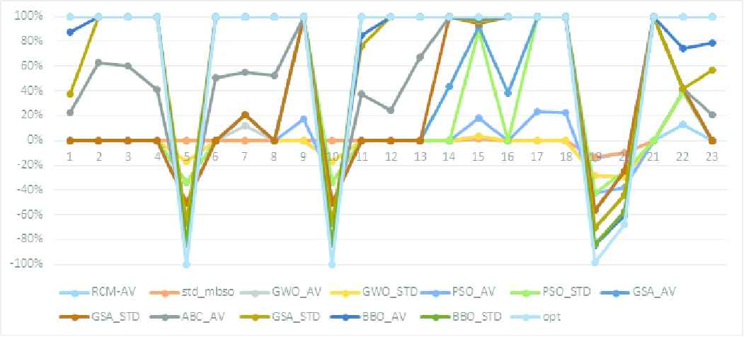
Unimodal benchmark function for Red Colobuses Monkey (RCM) with other algorithms.
5.2. Exploration Analysis
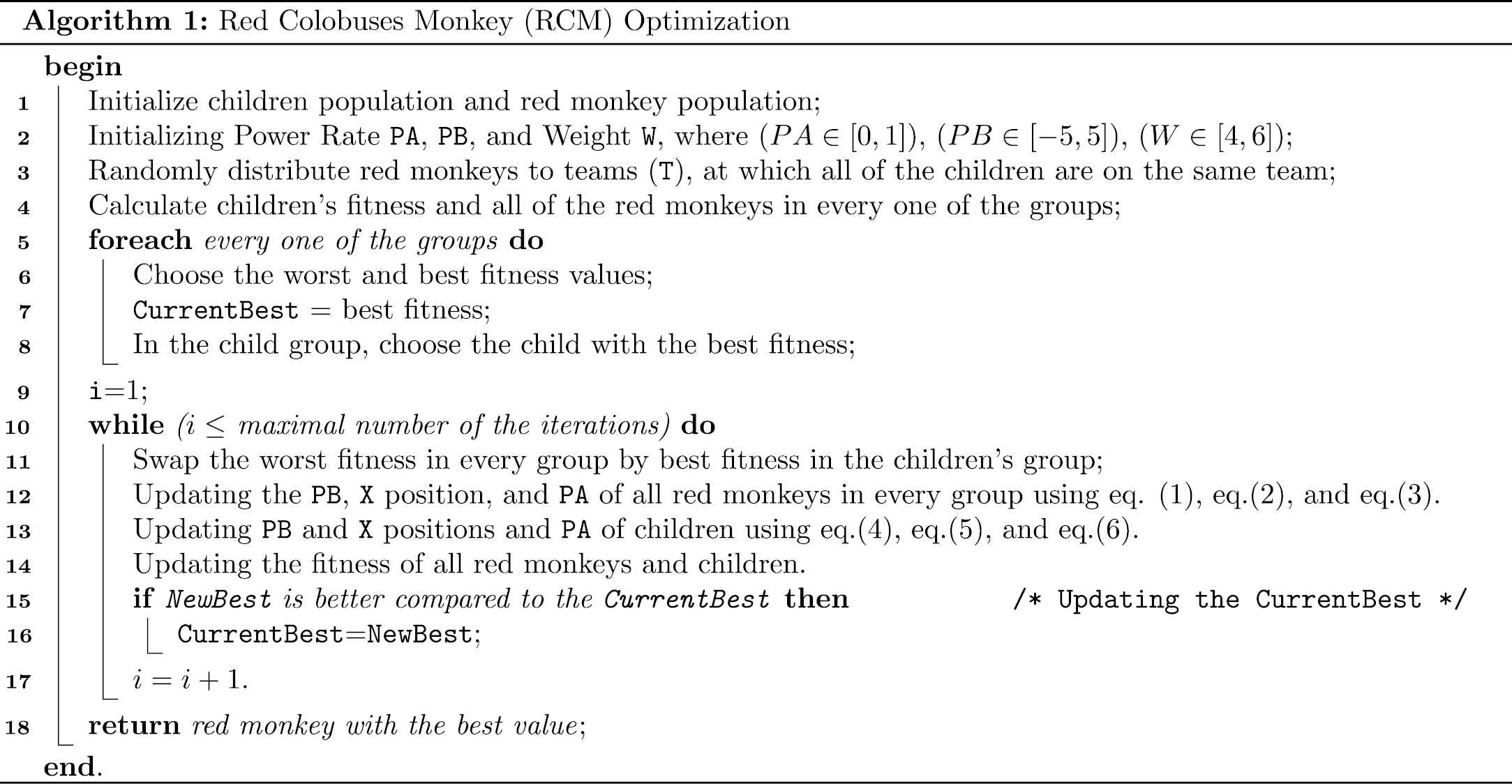
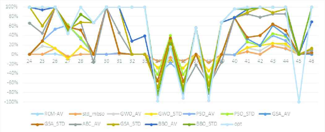
In the multimodal functions, various local optima could be recognized, with the number increasing exponentially with the dimension. Thus, multimodal functions were suitable to test the algorithm's exploration strength. Also, results in the Tables 5 and 6 showed that RCM is outperforming GWO, GSA, ABC, and PSO in the majority of the chosen 41 functions for multimodal functions (not fixed and fixed). The RCM in multimodal functions (not fixed) is similar to BBO and sometimes even outperforming it. The acquired results show the superiority of RCM concerning exploration; Figures 2 and 3 show a comparison regarding the average value of the multimodal benchmark functions between RCM, ABC, BBO, GWO, and PSO.
| RCM |
ABC |
PSO |
||||
|---|---|---|---|---|---|---|
| Function | Average | Std | Average | Std | Average | Std |
| F24 | −2.02E+00 | 4.60E–16 | −7.85E+102 | 1.75E+103 | −1.8758 | 0.2775018 |
| F25 | 8.88E–16 | 1.02E–31 | 0.0003463 | 0.0001776 | 1.95E–15 | 1.66E–15 |
| F26 | 4.20E–10 | 7.08E–12 | 0.5423613 | 0.4570343 | 1.19E–08 | 1.94E–08 |
| F27 | 0.0141401 | 0.204522 | 0.0089275 | 0.00297 | 0.6950133 | 0.7717305 |
| F28 | −1.0316 | 4.60E–16 | −1.0316 | 6.78E–16 | 15.759714 | 0.0088599 |
| F29 | 3 | 9.19E–16 | 3 | 0 | 3 | 0.4632838 |
| F30 | −6111.09 | 782.48996 | −1.20E+119 | 6.05E+119 | −3262.1366 | 0.059923 |
| F31 | 2.36E–31 | 4.53E–47 | 1.75E–07 | 1.67E–07 | 14.018373 | 3246.0832 |
| F32 | 1.35E–32 | 2.83E–48 | 5.12E–07 | 6.48E–07 | 1.35E–32 | 4.45E–47 |
| F33 | 2.05E–93 | 0 | 2.50E–09 | 2.06E–09 | 2.27E–100 | 5.57E–48 |
| F34 | 0 | 0 | 3.18E–05 | 2.96E–05 | 2.96E–17 | 3.57E–05 |
| F35 | −106.7645 | 1.47E–14 | −106.7645 | 7.23E–14 | −103.11511 | 5.78E–17 |
| F36 | −2.0626 | 4.60E–16 | −2.0626 | 1.36E–15 | −2.0623387 | 19.988736 |
| F37 | −0.6737 | 2.30E–16 | −0.67367 | 0 | −0.6737 | 0 |
| F38 | −952.47733 | 1.3805245 | −6.38E+111 | 2.29E+112 | 95.542387 | 0 |
| F39 | −19.2085 | 0 | N/A | N/A | −15.140224 | 0 |
| F40 | 2.546E–05 | 0 | −1.97E+113 | 1.03E+114 | 711.51431 | 5.42E–15 |
| F41 | −1.8013 | 4.60E–16 | −1.8788467 | 0.0784205 | −1.8010867 | 447.09172 |
| F42 | 0.0112751 | 0.019188 | 1.04E–05 | 2.86E–06 | 3.00E–15 | 0.0003598 |
| F43 | 1.11E–29 | 3.36E–30 | 15.67116 | 8.5558629 | 1.22E–29 | 1.76E–30 |
| F44 | 0.2999 | 0 | 0.364346 | 0.0534167 | 0.27762 | 0.0702805 |
| F45 | 0 | 0 | −5.26E+104 | 7.12E+88 | 0.3054 | 0.52373 |
| F46 | 1.30E–31 | 2.86E–31 | 0.0002641 | 6.57E–05 | 4.07E–31 | 5.57E–31 |
| BBO |
GSA |
GWO |
||||
| Function | Average | Std | Average | Std | Average | Std |
| F24 | −2.0218 | 0 | −5.12666 | 0.0008961 | −2.0218 | 0 |
| F25 | 4.74E–09 | 1.64E–08 | 1.71E–10 | 1.07E–10 | 8.88E–16 | 4.01E–31 |
| F26 | 1.0636183 | 0.2073279 | 2.23E–17 | 5.39E–18 | 0.551828 | 0.3234955 |
| F27 | 0.0014383 | 0.0009173 | 0.0044705 | 0.0020576 | 0.0009717 | 0.0009025 |
| F28 | −1.0316 | 6.78E–16 | −1.0316 | 6.78E–16 | −1.0316284 | 4.31E–09 |
| F29 | 3 | 0 | 3 | 0 | 3.0000079 | 9.28E–06 |
| F30 | −8198.7707 | 572.13167 | −2841.2 | 399.65132 | −6095.8133 | 790.14897 |
| F31 | 1.91E–10 | 4.11E–10 | 3.16E–21 | 2.91E–21 | 1.45E–08 | 1.50E–08 |
| F32 | 3.41E–12 | 1.70E–11 | 1.84E–21 | 1.57E–21 | 1.48E–08 | 1.90E–08 |
| F33 | 0.0398187 | 0.1032536 | 6.25E–21 | 7.71E–21 | 0 | 0 |
| F34 | 0.065493 | 0.1017525 | 0 | 0 | 0 | 0 |
| F35 | −106.11605 | 3.5517252 | −106.7645 | 7.23E–14 | −106.11607 | 3.5517344 |
| F36 | −2.0626 | 1.36E–15 | −2.0626 | 1.36E–15 | −2.0626119 | 3.30E–09 |
| F37 | −0.519266 | 0.1923383 | −0.6708967 | 0.0041723 | −0.6737 | 1.13E–16 |
| F38 | −791.28165 | 147.33382 | −727.02819 | 123.86803 | −922.42745 | 208.90989 |
| F39 | −18.88504 | 1.7716634 | −19.179587 | 0.0424768 | −19.208493 | 8.18E–06 |
| F40 | 46.717473 | 64.847441 | 206.868 | 81.44366 | 59.219524 | 74.583411 |
| F41 | −1.8013 | 1.07E+02 | −1.8013 | 6.78E–16 | −1.8013 | 6.78E–16 |
| F42 | 1.10E–11 | 1.95E–11 | 1.54E–11 | 2.86E–06 | 0 | 0 |
| F43 | 0.002171 | 0.0018676 | 6.59E–17 | 8.5558629 | 3.3787 | 4.1156058 |
| F44 | 0.19987 | 0 | 0.285 | 0.0534167 | 0.0999 | 0 |
| F45 | 0 | 0 | 0.01294 | 7.12E+88 | 0 | 0 |
| F46 | 2.86E–12 | 3.55E–12 | 3.74E–22 | 6.57E–05 | 2.14E–09 | 5.83E–10 |
ABC, Artificial–Bee–Colony; BBO, Biogeography–Based Optimizer; GSA, Gravitational Search Algorithm; PSO, Particle Swarm Optimization; RCM, Red Colobuses Monkey
Results of multimodal benchmark functions (not fixed).
| RCM |
ABC |
PSO |
||||
|---|---|---|---|---|---|---|
| Function | Average | Std | Average | Std | Average | Std |
| F47 | 7.02E–108 | 1.50E–107 | 6.67E–10 | 5.56E–10 | 1.67E–41 | 2.27E–41 |
| F48 | 0.3979 | 1.15E–16 | 0.39789 | 1.69E–16 | 0.482471 | 91.465336 |
| F49 | −3.8628 | 9.19E–16 | −3.8628 | 3.16E–15 | −3.8627821 | 0 |
| F50 | −3.3224 | 1.38E–15 | −3.3224 | 1.36E–15 | −3.2704748 | 1.36E–15 |
| F51 | −195.629 | 0 | −195.629 | 5.78E–14 | −195.62902 | 8.67E–100 |
| F52 | −1 | 0 | −1 | 0 | −1 | 0.0014962 |
| F53 | −50 | 0 | −49.997403 | 0.0024609 | −50 | 1.13E–16 |
| F54 | −0.869 | 2.30E–16 | −2.8739 | 9.03E–16 | 0.0625 | 376.90308 |
| F55 | −2081.5926 | 2747.1414 | −2.73E+116 | 3.91E+100 | 43.40452 | 193.60026 |
| F56 | 1 | 0 | 1.00044 | 0.0002408 | 1 | 0 |
| F57 | 0 | 0 | 2.58E–06 | 2.67E–06 | 0 | 0 |
| F58 | 0.1331051 | 0.031829 | 5.08E–06 | 2.76E–06 | 21.39248 | 22.479063 |
| F59 | −24776.518 | 3.77E–12 | −24776.516 | 0.0036263 | −24777 | 0 |
| F60 | 0 | 0 | 1.29E–06 | 9.74E–07 | 1.43E–103 | 3.20E–103 |
| F61 | 0 | 0 | 5.03E–05 | 3.29E–05 | 4.73E–31 | 4.32E–31 |
| F62 | 1.35E–31 | 4.53E–47 | 5.97E–07 | 4.52E–07 | 1.35E–31 | 0 |
| F63 | −0.8026685 | 1.5316153 | −384.9026 | 193.93391 | −0.6411 | 0 |
| F64 | 1 | 0 | 7.76328 | 0.5372398 | 1.8879 | 2.48E–16 |
| F65 | 0.0027813 | 4.14E–05 | 0.0077256 | 0.0023395 | 0.0017367 | 0.0018951 |
| BBO |
GSA |
GWO |
||||
| Function | Average | Std | Average | Std | Average | Std |
| F47 | 7.42E–09 | 4.23E–09 | 7.84E–18 | 5.56E–10 | 5.96E–120 | 9.10E–120 |
| F48 | 0.39789 | 1.69E–16 | 0.3979 | 0 | 0.3978879 | 5.98E–07 |
| F49 | −3.8628 | 3.16E–15 | −3.8627967 | 1.83E–05 | −3.8620812 | 0.001938 |
| F50 | −3.27472 | 0.0593941 | −3.3224 | 1.36E–15 | −3.2642539 | 0.0998765 |
| F51 | −195.629 | 5.78E–14 | −195.629 | 5.78E–14 | −195.62903 | 2.85E–08 |
| F52 | −1 | 0 | −1 | 0 | −1 | 0 |
| F53 | −50 | 0 | −50 | 0 | −49.99989 | 8.03E–05 |
| F54 | −0.769653 | 0.1456735 | −0.869 | 1.13E–16 | −0.869 | 1.13E–16 |
| F55 | −6.1295 | 0 | −4035.32 | 3.91E+100 | −12266.82 | 6663.9663 |
| F56 | 1 | 0 | 1 | 0.0002408 | 1 | 0 |
| F57 | 1.67E–06 | 1.88E–06 | 2.75E–20 | 2.67E–06 | 6.44E–08 | 5.08E–08 |
| F58 | 0.0948764 | 0.0142888 | 0.10288 | 2.76E–06 | 0.14548 | 0.0329826 |
| F59 | −24776.518 | 0 | −39.6307 | 0.0036263 | −24777 | 0 |
| F60 | 1.03E–14 | 2.31E–14 | 2.45E–19 | 9.74E–07 | 0 | 0 |
| F61 | 2.06E–14 | 4.59E–14 | 2.56E–19 | 3.29E–05 | 5.80E–06 | 6.32E–06 |
| F62 | 2.06E–14 | 4.60E–14 | 3.37E–20 | 4.52E–07 | 1.07E–07 | 9.60E–08 |
| F63 | −1.9105 | 0 | −1.91022 | 193.93391 | −1.9105 | 0 |
| F64 | 1.01135 | 0.0014387 | 1 | 0.5372398 | 1.23078 | 0.0955472 |
| F65 | 0.0008756 | 0.0002102 | 0.0005661 | 0.0023395 | 0.0014036 | 0.0007647 |
ABC, Artificial–Bee–Colony; BBO, Biogeography–Based Optimizer; GSA, Gravitational Search Algorithm; PSO, Particle Swarm Optimization; RCM, Red Colobuses Monkey.
Results of multimodal benchmark functions (fixed).
Multimodal benchmark function (not fixed) for Red Colobuses Monkey (RCM) with other algorithms.
Multimodal benchmark function (fixed) for Red Colobuses Monkey (RCM) with other algorithms.
Based on the results of unimodal test functions shown in Table 4, RCM achieves optimum value in 7 test functions (F5, F6, F7, F10, F12, F14, and F16). In contrast, it converges to optimal values in 8 test functions (F1, F11, F13, F15, F18, F19, F20, and F22). It must be indicated that such values were better in comparison to values regarding other chosen algorithms utilizing identical testing functions.
RCM results are showing that it is effective and competitive in comparison to the algorithms mentioned above. Also, it is superior to them in the majority of tests. Such results also showed the accuracy, flexibility, and efficiency of the RCM in exploitation means of view.
According to the results which were provided in the Table 5 containing a multimodal test (not–fixed), RCM achieves optimal value in 6 test functions (F27, F28, F33, F36, F38, and F40). In contrast, it was too close to optimal values in 3 test functions (F34, F35, and F37). It must be indicated that the values which are close to optimal in 5 test function (F26, F41, F42, F43, and F44) were better in comparison to the values of other algorithms utilizing identical testing functions. Concerning the rest 9 test functions (F21, F22, F28, and F43), RCM can be close to the best values regarding the chosen algorithms.
According to the results which have been reached, the optimal value in twelve test functions (F47, F48, F49, F50, F51, F52, F53, F56, F57, F60, F61, and F64), whereas it was too close to optimal values in 3 test functions (F54, F58, and F59), it must be indicated that the values were better in comparison to values of the rest of the chosen algorithms utilizing the same testing functions. Furthermore, in the rest 3 test functions (F55, F62, and F63), RCM can be close to the chosen algorithms' best values.
The findings indicate that in contrast to the unimodal performance, RCM achieves excellent results in detecting the optimal solution value in a multimodal function, suggesting that the RCM has been superior in the exploration search.
6. CONCLUSION AND FUTURE WORK
This study provided a new nature–inspired metaheuristic algorithm based on the social behavior of Red Colobuses Monkey. Also, RCM is proposed as an approach used for solving optimization problems. In RCM, the solutions have been essential for upgrading their positions based on the optimal solution, which was achieved thus far. RCM can also replace the worst red monkey by the best child identified, thus improving solutions. Updating the position allows a solution for moving outwards or towards the destination point to ensure exploration and exploitation of search space. Overall, 64 test functions were used to test the effectiveness and power of RCM concerning exploration and exploitation. The obtained results showed that RCM is superior to BBO, GSA, ABC, and GWO, while the results acquired from unimodal test functions indicated the RCM's exploitation superiority. Then, the exploration ability of RCM is shown via the results acquired from multimodal benchmark functions. Furthermore, RCM might solve different optimization problems (parameters optimization, maintenance, scheduling, and many others).
Many research directions might be suggested for studies with the suggested algorithm, such as to build a multiobjective type of RCM algorithm and solve various optimization problems.
CONFLICTS OF INTEREST
The authors have declared no conflicts of interest.
REFERENCES
Cite this article
TY  - JOUR
AU  - Wijdan Jaber AL-kubaisy
AU  - Mohammed Yousif
AU  - Belal Al-Khateeb
AU  - Maha Mahmood
AU  - Dac-Nhuong Le
PY  - 2021
DA  - 2021/03/17
TI  - The Red Colobuses Monkey: A New Nature–Inspired Metaheuristic Optimization Algorithm
JO  - International Journal of Computational Intelligence Systems
SP  - 1108
EP  - 1118
VL  - 14
IS  - 1
SN  - 1875-6883
UR  - https://doi.org/10.2991/ijcis.d.210301.004
DO  - 10.2991/ijcis.d.210301.004
ID  - AL-kubaisy2021
ER  -