
Abnormal Traffic Detection Based on Generative Adversarial Network and Feature Optimization Selection
- DOI
- 10.2991/ijcis.d.210301.003How to use a DOI?
- Keywords
- Abnormal traffic detection; Generative confrontation network; Collaborative learning automata; Multicore maximum mean difference; Softmax
- Abstract
Complex and multidimensional network traffic features have potential redundancy. When traditional detection methods are used for training samples, the detection accuracy of the supervised classification model is affected due to small data samples. Therefore, a method based on generative adversarial networks (GANs) and feature optimization is proposed. First, the feature correlation and redundancy are analyzed by the potential redundancy of network traffic. The feature optimization selection method of collaborative learning automata is proposed. Second, the confrontation interactive training principle of the generative confrontation network is adapted, in which a model of the generative confrontation network is proposed to solve the problem that small training label samples. Third, the interdomain distance is minimized by using GAN and the multiple kernel variant of maximum mean discrepancy (MK-MMD). The shared features between the source domain and target domain distribution are learned by applying the information between GAN confrontation training and classification network supervision training, improving the detection accuracy. Forth, random noise data and original training label samples are mixed to form a new training set. The accuracy is further improved by adopting generative models to continuously generate samples. The final classification results are output by the 16-dimensional Softmax classifier. The method has a small loss rate when the datasets are used to train by the experimental analysis of algorithm parameters and simulation data. The model optimized by MK-MMD has strong generalization ability. The average detection accuracy rates are 91.673% (two-classification) and 91.480% (multiclassification) by comparing machine learning and other shallow neural networks, and are the highest values among the compared methods. Moreover, the effectiveness and superiority of the proposed method are verified to be the best by comparing the recall rate, false positive rate (FPR), F-measure, AUC. When the interference of other samples are mixed, the proposed method is also robust.
- Copyright
- © 2021 The Authors. Published by Atlantis Press B.V.
- Open Access
- This is an open access article distributed under the CC BY-NC 4.0 license (http://creativecommons.org/licenses/by-nc/4.0/).
1. INTRODUCTION
With the rapid development of network technology, intelligent network technology has played an important supporting role in promoting sustainable economic and social development [1–3]. The rapid development of network technology has made the network structure increasingly complex. This has given rise to increasing risks of network intrusions and abnormal traffic attacks. Such risk is an additional problem that must be solved as the network moves toward future sustainable development. The analysis and identification of various network intrusions are highly important [4,5]. Abnormal detection technology has had to face increasing challenges due to the increase in network size, network speed and types of intrusions. Therefore, design of new abnormal detection mechanism for the current and future network environment is the core subject of research in network-related fields [6,7]. Moreover, the abnormal detection method must increase the speed of abnormal detection, reducing the false positive rate (FPR) and improving the detection performance. For different network environments, many detection methods have been proposed. Meanwhile, the researches on network abnormal detection are the essential problem in the network space. Researches on such information processing problems are usually carried out on the tagged dataset. The validity of the algorithm is verified by the tagged data. However, this is different from the information that ordinary technicians can process directly, such as images and sounds. Network traffic information is highly abstract professional data which require trained experts. Due to the high threshold of network abnormal sample labeling, small datasets are used for network abnormal detection, posing challenges to the research on network abnormal detection. On the other hand, in the real environment, a real-time response is required for new network abnormal detection methods. There is usually not enough time to mark a large number of abnormal samples. Therefore, the design of a method for small sample field detection [8,9] is also the most important.
In the view of the potential redundancy of the traffic features of complex networks, traditional detection methods have the disadvantage that the detection accuracy of the supervised classification model is affected by the lack of samples. In this paper, based on the optimal selection of features, a network abnormal traffic detection method is proposed in combination with the generative adversarial networks (GAN) and multiple kernel variant of maximum mean discrepancy (MK-MMD). The contributions are mainly divided into three sections:
After analyzing the feature correlation and redundancy, a feature optimization method of the collaborative learning automata (LA) is proposed. The problem of too many redundant features in abnormal traffics are solved by finding the optimal feature subset from the features with a collaborative LA.
Based on the principle of GAN interactive training, an abnormal detection model of GAN is proposed to solve the problem of low detection accuracy due to the small number of training label samples.
The MK-MMD is proposed to minimize interdomain distance. The information between the confrontation training and the classification network supervision training of GAN are optimized. The shared features between the distribution of source domain and target domain are learned by the model. The detection accuracy has been further improved.
The remainder of this paper is organized as follows. The purpose of abnormal network traffic detection and the existing problems are introduced in Section 1, we summarize the research status of abnormal network traffic detection in Section 2. The theories and the implementations of abnormal traffic detection based on GAN, MK-MMD and feature optimization selection are described in Section 3. In Section 4, we evaluate our methods, and the relevant experiments are set up to verify the effectiveness of the proposed method. Section 5 concludes this paper.
2. RELATED WORKS
2.1. Feature Optimization Selection
Many studies have been performed on feature optimization selection. As shown in Ref. [10], a classic feature selection metric GeFS is optimized. Moreover, a filtering method for multiclassification feature optimization selection is proposed after combining it with the support vector machine (SVM) classifier. The feature selection problem is transformed into a mixed 0–1 linear programming problem by adopting the classifier. The SVM classifier is fused and applied to network traffic abnormal detection with good results. As shown in Ref. [11], an improved filtering feature optimization selection method is proposed, in which mutual information theory is applied to evaluate the correlation between each dimension of network traffic features and output classes. The feature selection algorithm is used to select the optimal feature to achieve abnormal traffic classification. Weka technology and voting mechanisms are adopted, in which a feature selection algorithm is proposed to filter features through the method. Moreover, each dimensional feature is rated by the voting mechanism, and the most effective feature in network traffic is screened out. Finally, various classifiers are used for abnormal detection to verify their effectiveness [12]. The network traffic features of the two datasets KDD99 and UNSW-NB15 have been fully studied, and the feature correlation rules have been extracted. A feature selection model of the association rule mining algorithm is proposed. Meanwhile, the highest ranking feature is mined from network traffic, and (EM) expectation- maximization clustering and naive Bayes classifier are combined to detect abnormal traffic in Ref. [13]. As shown in Ref. [14], LA is applied to the field of abnormal detection. A single LA interacts with a random environment in which redundant features are removed from the initial feature set to achieve feature space dimensionality reduction. Furthermore, the model is combined with SVM to improve the detection efficiency.
2.2. Abnormal Traffic Detection Based on Traditional Machine Learning
The traditional methods of machine learning include the K nearest neighbor algorithm (KNN), naive Bayes algorithm (NB), SVM, decision tree and random forest (RF) algorithm. The core concept of the KNN algorithm is to calculate the distance between the test sample and the training sample in the feature space. Then, the K most adjacent training sample nodes are selected and grouped into a category. The idea of the NB is based on Bayes’ theorem and the independent conditional hypothesis to complete the classification according to probability mode. However, these two detection techniques need to give a score or probability of whether a particular event is an exception. The abnormal detection system must aggregate the output, leading to a high FPR. Therefore, an abnormal detection method has been studied and designed to optimize Bayesian networks to solve this problem in Ref. [15]. By combining RF with Bayesian optimization, information gain is utilized to select key factors of production. Sensitivity analysis is used to optimize the classification effect. Meanwhile, the outputs of k different detection models and optionally additional information were output. Each model analyzed different features of events. Finally, the logical model combination of various output parameters were returned, and the Bayesian network was used to complete the classification. The shape of the description in the normal data is presumed by the SVM. The correct acceptance rate of the given normal sample is guaranteed by minimizing the volume based on the given empirical error.
However, the standard SVM model needs to contain annotated data. The original SVM is no longer applicable because there is only one class of samples. Therefore, a one-class SVM method for exception detection is proposed. It assumes that the coordinate origin is a unique constant point and that a hyperplane is found to separate the sample point from the origin to the maximum extent. All of the sample points fall on one side of a semi hyperplane, while the other sample points are considered anomalies [16]. However, when the area of half space is too large, the FPR is higher. Therefore, the Slab SVM method was proposed by Ref. [17] to solve this problem by constraining the sample points between two parallel hyperplanes. The samples can be better classified in the stripe form. The decision tree algorithm is a common algorithm in the field of machine learning that finds an optimal value from a dataset based on probability. The optimal value is divided into two datasets, and the optimal value is found from the dataset. RF is a classification algorithm in which multiple decision trees are used for training. Moreover, to solve the problem of the lack of precision of the RF algorithm element classifier, a gradient promotion decision tree as a meta-classifier of the database abnormal detection algorithm was studied [18]. While the classification accuracy was improved, it can resample the original dataset, and the correlation of noise data can be weakened. The overfitting of a single element classifier can be filtered by the random voting mechanism in the model.
Furthermore, the D Flow model is used to reduce the record of network traffic, and four features of traffic are extracted to capture abnormal traffic behavior in Ref. [19]. The redundant features in the traffic are filtered by a scale space filter. The threshold of the filter is selected according to the system criteria to evaluate the degree of abnormality. The influence of different traffic features on the detection of abnormal behavior is experimentally analyzed. Abnormal behavior unrelated to traffic change can be detected effectively by this method, and the detection accuracy is relatively high. As shown in Ref. [20], a dynamic threshold method is used to detect network traffic anomalies. First, an adaptive threshold is used to calculate some parameters of network traffic features. Then, four different attributes of important feature calculation in traffic are extracted and used for DDoS detection. When the attribute calculated within a certain time interval is greater than the threshold value, the attribute is regarded as an attack. Since this approach relies on the optimal selection of the threshold value, and it is highly limited.
2.3. Abnormal Traffic Detection Based on Deep Learning
Although the traditional machine learning algorithms can help identify some attacks, the task of two-classification and multiclassification under small data cannot be solved effectively. In recent years, the potential of deep learning algorithms have been demonstrated in many fields. The progress in related fields can be rapidly driven by this technique because it provides an effective approach to solve the feature design problem of traditional machine learning. Ref. [21] proposed the abnormal detection method of a convolutional neural network (CNN), and the learning method of image transformation was adopted to realize abnormal detection. First, the discrete data are transformed into one-hot vector to achieve vectorization. Then, the features are folded and arranged to realize data conversion from one dimension to three dimensions. Finally, ResNet and Google Net are used to conduct classification experiments on the NSL-KDD dataset, and the model performance is verified. Ref. [22] studied a recurrent neural network (RNN) abnormal traffic detection. First, the vectorization of discrete data and normalization of all data are carried out. Then, the feature extraction and classification of preprocessed data are carried out using a RNN. The advantages of two-classification and multiclassifications for the NSL-KDD datasets are verified by experiments. Ref. [23] designed a RNN with feature grouping for abnormal detection that improved the speed of training and convergence by adjusting the size of the network. Therefore, this model becomes a more efficient abnormal detection system in terms of accuracy rate (Acc)and operation cost. Ref. [24] proposed a deep automatic encoder to detect abnormal traffic. The autoencoder is used to complete data dimension reduction and improve the performance of the abnormal detection system. Experiments with the NSL-KDD dataset show better accuracy for this approach compared to the other methods. Ref. [25] designed an abnormal detection system based on a deep belief networks (DBN) that trained the model with the NSL-KDD dataset to identify unknown attacks. The accuracy of the detection model is high, and it can detect the abnormal traffic well compared to the other methods. A SVM abnormal detection model based on self-coding networks was proposed by Ref. [26]. In the pretraining stage, the self-coding network method is used to extract the low-dimensional feature representation of the data, and the SVM classification algorithm is used for abnormal identification. The training time of the classification model is reduced by using this detection method, and the classification effects are better than that of the traditional algorithm. As shown in Ref. [27], each network traffic is represented as a state set that changes over time, and then the RNN is used to model and complete the detection of abnormal network traffic. However, this paper does not study the traffic feature modeling method to detect botnets, so that it also displays some limitations. As shown in Ref. [28], a stack noise reduction self-encoder abnormal detection method was proposed that can effectively improve the accuracy and robustness of traffic feature analysis of big data. Moreover, the additional computational burden incurred by traffic conversion to images is avoided, but (SDA) stacked denoise autoencoder has only three hidden layers. Therefore, the feature extraction and dimension reduction capability of SDA cannot be exploited well, affecting the model detection performance.
Furthermore, a network abnormal detection algorithm for the optimized and improved regularized limit learning machine (BSO-IRELM) is studied in Ref. [29]. First, LU decomposition is used to solve the output weight matrix of RELM. Then, the long-run optimization algorithm is designed to jointly optimize RELM weights and thresholds. Finally, the detection performance of the model is verified on multiple datasets. In Ref. [30], a C-LSTM neural network is proposed that can effectively model the space-time information contained in network traffic, and the model after modeling is used to extract traffic features. Although this method is effective for feature extraction of a time series network, the use of LSTM results in overfitting. A robust feature method for automatically extracting spatial and temporal information is provided to optimize the detection of abnormal network behaviors. The model has a high accuracy according to Ref. [31]. The high accuracy of combining CNNs, LSTM and deep neural networks (DNNs) to extract more complex network traffic features has also been proven by Ref. [32].
In summary, it can be observed that deep learning can effectively solve some problems in abnormal network traffic detection, so it is also the research direction of this paper.
2.4. Description of the Classification of Small Samples and the Idea of the Proposed Method
Description of the work above: for a specific type of attack, if there are a large number of samples, many machine learning algorithms can identify the corresponding attacks. This process can be learned automatically by deep learning methods without significant manual intervention. Thus, it can be concluded that as long as there are enough new datasets, the abnormal detection system can detect new attacks. However, the current cyberspace environment is evolving rapidly, with new attacks occurring every moment. For example, a zero-day attack is an attack launched on the day vulnerability is discovered, and it is difficult for security agencies to obtain enough attack samples in a short time. Meanwhile, there is no time to produce the dataset for release. The detection problem of similar zero-day attacks can be considered an abnormal detection problem in a small sample scenario [33].
In recent years, small sample learning has achieved some significant results. In particular, some small sample learning problems have been well solved by methods based on meta-learning [34] and metric learning [35]. However, for network abnormal detection, no effective detection algorithms suitable for small sample scenarios are currently known. As network attacks emerge ceaselessly, the existing supervised learning algorithms are difficult to generalize to identify unknown abnormal traffic. On the other hand, computer networks have become very popular. It is impractical to design a corresponding abnormal detection model for each type of business network and possible abnormal types. There are still many limitations in feature optimization selection and classification judgment. The overall network samples are directly inputted into the classifier for big data training in these studies. The final detection effects are poor due to the large-scale network environment with complex features and various attack categories.
Therefore, our improvement ideas are mainly as follows: first, the redundancy of network traffic is analyzed, and the collaborative LA is used for feature optimization selection. Then, the GAN network with MK-MMD is used to minimize the interdomain distance to improve the classification detection accuracy based on the GAN confrontational interactive training principle. Finally, the random noise data generated samples (fake samples) are mixed with the original training label samples to form a new training set, in which the detection accuracy in the small samples is further improved. Moreover, the effectiveness and robustness of the model are verified by the experiments.
3. IMPROVEMENT METHODS
The process of the proposed generation of the confrontation network and feature optimization selection detection model is shown in Figure 1. After the datasets are normalized, the variance of the feature value of the traffic will be reduced. All of the original data will be transformed into dimensionless numerical data. Step 1: after the network datasets are normalized, the output
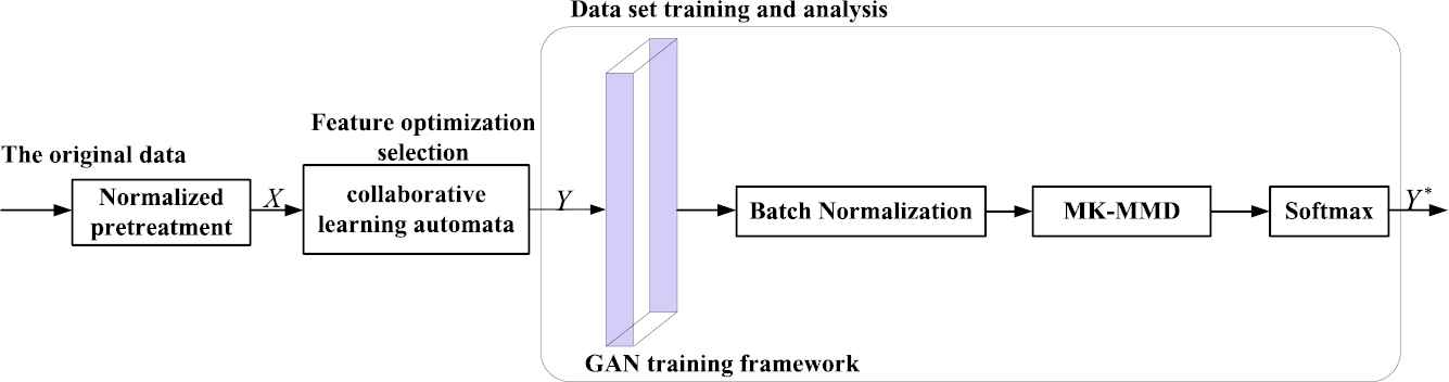
The overall inspection model structure process.
3.1. Feature Optimization Selection Based on Collaborative LA
The network traffic features can be divided into different types according to their features, such as basic features, content features and time features. The initial feature set can be divided into
At time
Action:
The behavior set of each
Feedback:
The feedback of the random environment is binary, where 0 represents reward, 1 represents punishment. The update strategy is the RI strategy. The probability of the behavior set is updated only if the feedback is a reward. Otherwise, it does not respond. In the proposed
Environment:
The random environment is responsible for responding to the selected set of behaviors at each iteration and returning feedback from the
However, a single
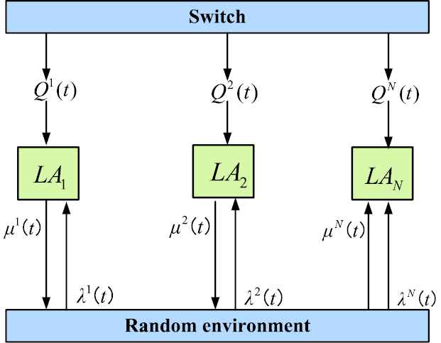
The principle of collaborative learning automata (LA).
The collaborative LA model is proposed and aims to adopt multiple
They have their probabilistic choice vectors
Algorithm 1: collaborative LA
Input:
Step 1 Initialization: Behavior probability vector:
Repeat
Step 2 At time
Step 3 The behavior set
Step 4 According to the currently selected behavior set
Step 5
Step 6 Until
It is observed that the collaborative LA can achieve convergence of
Therefore, the specific feature optimization selection algorithm that uses the aforementioned analysis process is as follows: in each iteration, each
The specific traffic chart of the optimization model is shown in Figure 3.
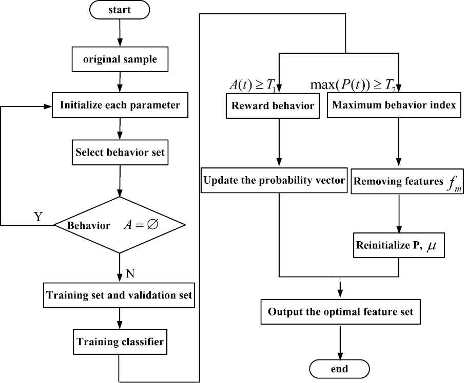
Feature optimization selection algorithm traffic.
3.2. Generative Countermeasure Network Optimization Detection
The model is based on a game theory scenario. The generator (
The structure diagram of the GAN model is shown in Figure 4 and is composed of two sections: the generator
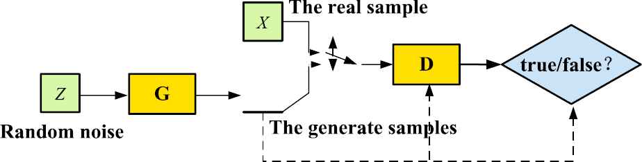
The sample structure diagram of the generated confrontation.
In this formula,
To make full use of unlabeled samples to assist in supervised learning training classification, the total loss function is decomposed into two sections: standard supervised learning
In Equation (4):
3.3. Framework Construction
The GAN detection framework is shown in Figure 5. The framework is composed of three sections: a feature optimization selector, generator
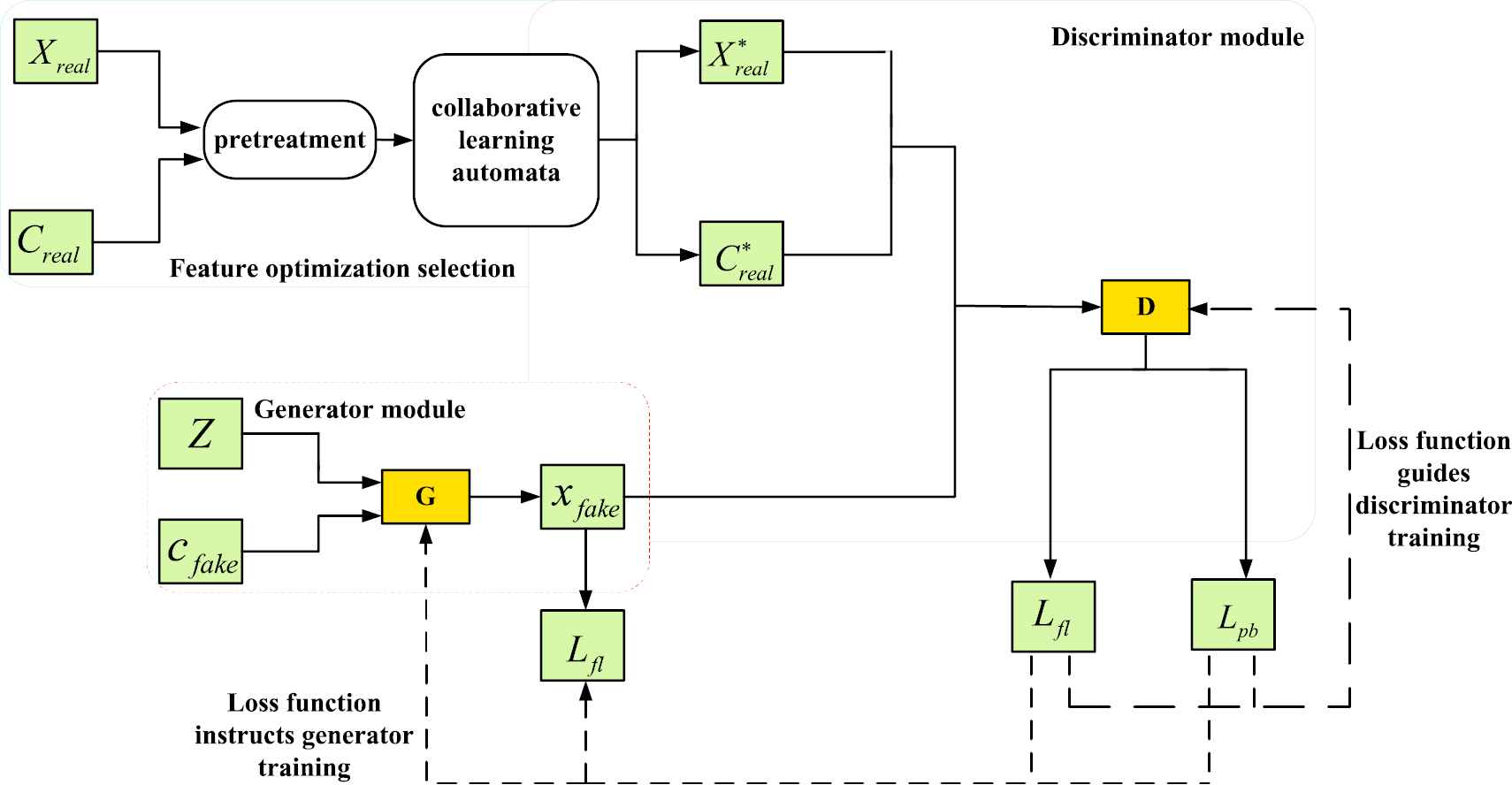
Generative adversarial networks (GAN) detection structure diagram.
To generate samples with specified semantics, the labels of the generated samples must be controlled. Therefore, the category data are imported into
3.4. Loss Function Derivation
The adversarial samples are added to GAN training that can use the advantages of GAN in deep learning to improve classification robustness. Meanwhile, the optimization efficiency of GAN can also be improved.
The function of the generator
The generator
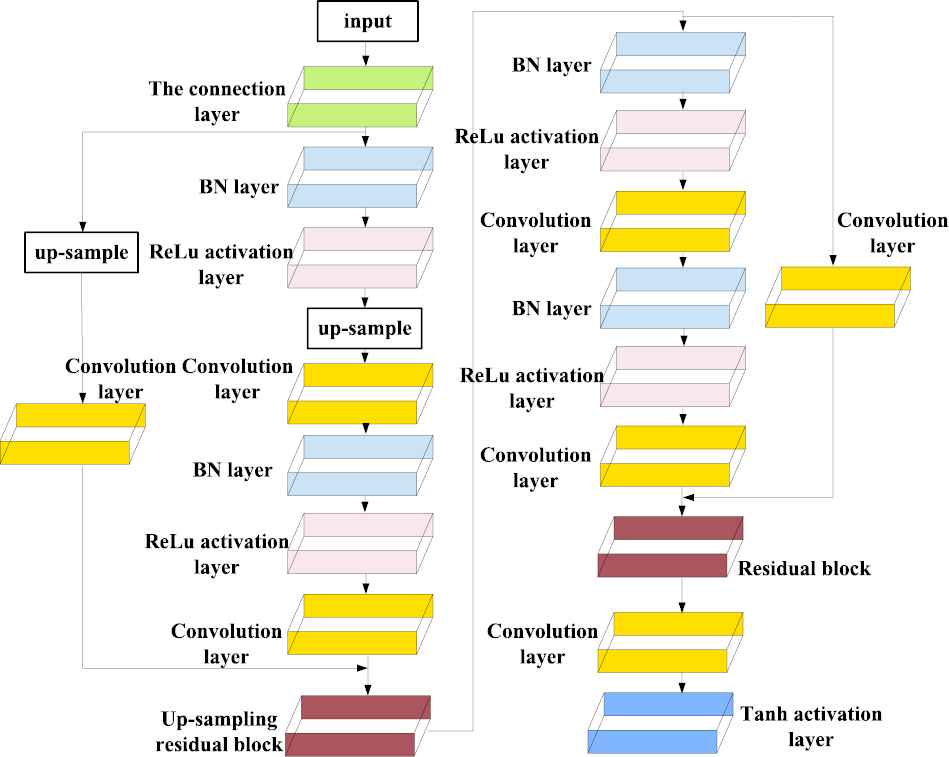
Structure diagram of generator G.
The D ability to distinguish real and false samples during training will be improved. In the training process, the weights of
The loss function
D is trained for the classification of various samples under the guidance of
The specific model of the designed discriminator
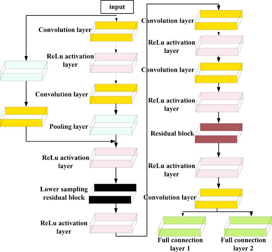
Structure diagram of discriminator D.
Just like generators, the deconvolution is removed, and only the ordinary convolutional layer is retained. The up sampling and down sampling are implemented through upSampling2D and avgPooling2D. The size of convolution kernel is uniformly 3×3, and the step size is 1. Because the normalization adds interdependencies among different samples in a Batch, the proposed method requires a gradient penalty for each sample. So BN is not used in the discriminator's model. Other parameters related to the generator and discriminator are described in Table 2.
| Model | Layer | Structure | Output |
|---|---|---|---|
| generator | 1 | Linear+Batch Normalization+ReLU | 128 |
| 2 | Linear+Batch Normalization+ReLU | 256 | |
| 3 | Linear+Batch Normalization+ReLU | 512 | |
| 4 | Linear+Batch Normalization+ReLU | 1024 | |
| 5 | Linear | 41 | |
| discriminator | 1 | Linear+ReLU | 128 |
| 2 | Linear | 2 |
Structure of generator and discriminator.
3.5. Multicore Maximum Mean Difference Optimization
Some training samples in the data domain of the learning classifier will be missing. Therefore, the classifier needs to be assisted by the data of the relevant field of the learning task. The domain knowledge is “transferred” to the classifier that is used to construct the target field classifier and optimize the test samples of the target field. Although the source domain data are correlated with the target domain data, there are significant distribution differences. Therefore, the maximum mean difference (MMD) method is proposed to eliminate the influence of distribution differences. This method is composed of the following sections: Training set is
The minimized MMD is transformed into the optimization problem of the objective function. First, the feature space is found to make the data distribution less different. Then, the source domain and target domain samples are mapped to the feature space, in which the classifier can obtain better performance. Finally, the metric
In the formula,
4. EXPERIMENT AND RESULT ANALYSIS
4.1. Dataset and Preprocessing
The test platform of this system includes hardware equipment and software. The configuration parameters are mainly shown in Table 3.
| Hardware | Model |
|---|---|
| processor | Intel®CoreTMi7-6700HQ CPU@2.60GHz×8 |
| memory | 16G |
| GPU | GeForce GTX 960M/PCIe/SSE2 |
| hard disk | 1TB |
| operating system | Windows 10 |
| language | Python |
| IDE | Pycharm |
| framework | Keras |
GPU, graphic processing unit; IDE, integrated development environment.
The specific operating environment of the experiment.
The experimental dataset selected in this paper is the NSL-KDD dataset. Since it was proposed in 2009, the NSL-KDD dataset has been widely used in abnormal detection experiments. In recent studies, most researchers have used NS-KDD as dataset because this datasetS effectively solve the inherent data redundancy problem in the KDDCup99 dataset. The number of records was adjusted to make the number of records in the training set and test set reasonable. The laboratory simulates the local area network environment and simulates different network traffic, including normal traffic and various abnormal behaviors. This dataset contains a total of 9 weeks of traffic data that are divided into a training set and a test set. The training set consists of more than 5 million network connection records in the first 7 weeks that are stored as binary TCPdump compressed data. The TCPdump data exceeded 4 GB, and the test set included more than 2 million network connection records in the last 2 weeks.
Therefore, the “KDDTrain+” of NSL-KDD is selected as the training set. Meanwhile, the category label is removed. The “KDDTest+” is selected as the test set. Each dataset consists of 5 types of traffic: normal traffic and 4 types of attack traffic. The four types of attack traffic are: DoS, U2R, R2L, and Probe. The experiment mainly focuses on the effect of detecting network anomalies in terms of traffic. Therefore, only 28 features related to traffic in the dataset are retained. Moreover, the symbolic features are transformed into numerical features. The minimum-maximum normalization method is used to normalize the attribute values of 28-dimensional features. The traffic feature vector is constructed for the training of abnormal detection model. The detection of anomalous traffic is realized.
4.2. Performance Analysis of Collaborative LA Detection
Four sets of optimized feature subsets are experimented to verify the performance of the collaborative LA. The data is shown in Table 4. The four groups of feature subsets are respectively numbered LA1, LA2, LA3 and LA4. The LA1 and LA2 are composed of 10 feature dimensions. The LA3 and LA4 are composed of 9 feature dimensions. The results of abnormal detection is shown in Table 4. When using the feature optimization method and the nonfeature optimization method, the Acc and FPR are given.
| Numbering | Indicator | Normal | DoS | Probe | U2R | R2L |
|---|---|---|---|---|---|---|
| Not optimized | Acc (%) | 84.695 | 80.634 | 60.413 | 9.147 | 21.765 |
| FPR (%) | 11.238 | 15.369 | 34.917 | 88.964 | 72.417 | |
| LA1 | Acc (%) | 89.562 | 86.521 | 73.487 | 0 | 0 |
| FPR (%) | 8.347 | 10.234 | 22.109 | 100 | 100 | |
| LA2 | Acc (%) | 91.606 | 88.527 | 76.394 | 0 | 0 |
| FPR (%) | 6.524 | 8.631 | 19.336 | 100 | 100 | |
| LA3 | Acc (%) | 92.457 | 90.632 | 79.608 | 44.725 | 0 |
| FPR (%) | 4.419 | 6.528 | 15.455 | 50.369 | 100 | |
| LA4 | Acc (%) | 94.894 | 93.697 | 84.557 | 85.629 | 86.327 |
| FPR (%) | 2.065 | 2.636 | 10.603 | 9.701 | 8.624 |
FPR, false positive rate; LA, learning automata.
Comparison results of feature selection.
It is observed from Table 4 that when the collaborative learning automatic is not used to optimize the dataset, the detection accuracy of the normal traffic and the four types of attack traffics are low. The Acc of the normal traffic is 84.695%, while the detection Accs of U2R and R2L in the four attack traffics are only 9.147% and 21.765%, respectively. The average Acc of the four types of attack traffic is 35.339%, and the performance is poor. However, the optimal feature subset can be effectively selected from the NSL-KDD dataset through feature optimization selection based on collaborative LA. Meanwhile, this feature subset can have a positive effect on the Acc of the entire abnormal detection model. The accuracy of the overall abnormal detection will be improved. Meanwhile, Table 4 shows that the best-performing set of optimal feature subsets (LA4) has a detection accuracy of 94.894% for normal traffic. The average Acc of the four types of attack traffic is 87.553%, which is a great improvement over the previous performance. However, the feature subsets that are selected by the learning automatic are not necessarily same. It is observed that they have a higher Acc and a lower FPR than the initial feature set, also verifying the effectiveness of the proposed method. The proposed method and the feature optimization selection methods in recent years have been compared with experimental results to further verify the effectiveness of the collaborative LA method.
The evaluation results of different feature optimization selection methods are shown in Table 5. A feature subset containing 12 features are selected by the Weka model. A feature subset containing 14 features are selected by ARM technology. The feature subset is selected by S-LA contains 10 feature dimensions by a single learning automatic. The optimal feature subset containing 9 features are selected by the collaborative learning automatic.
| Dataset | Algorithm | Number | Feature Ranking | Accuracy |
|---|---|---|---|---|
| NSL-KDD | Weka | 12 | 2, 3, 5, 6, 11, 23, 24, 33, 34, 35, 36, 40 | 83.629% |
| ARM | 14 | 3, 7, 12, 15, 16, 20, 22, 30, 34, 36, 37, 358, 39, 41 | 86.364% | |
| S-LA | 10 | 3, 11, 12, 16, 19, 22, 27, 29, 32, 36 | 89.637% | |
| Proposed | 10(LA1) | 2, 3, 5, 6, 10, 29, 30, 32, 33, 34, 36 | 89.794% | |
| 10(LA2) | 2, 3, 5, 11, 29, 32, 33, 35, 36, 41 | 90.643% | ||
| 9(LA3) | 2, 3, 5, 10, 32, 33, 36, 37, 39, 41 | 91.752% | ||
| 9(LA4) | 2, 3, 5, 10, 29, 32, 33, 36, 41 | 93.871% |
Evaluation results of several feature optimization selection method.
It is observed from the above results that compared with other feature optimization selection methods, the proposed method can obtain higher accuracy of abnormal detection with a strong improvement in the Acc. Moreover, in terms of the feature dimension of the optimal feature subset, the feature dimension can be greatly reduced by the feature optimization selection method, in which more redundant features and irrelevant features are eliminated. The optimal feature subset with smaller feature dimensions can not only be obtained by the proposed method but also the detection efficiency of abnormal detection is improved.
4.3. Design and Analysis of the Training Set and Test Set
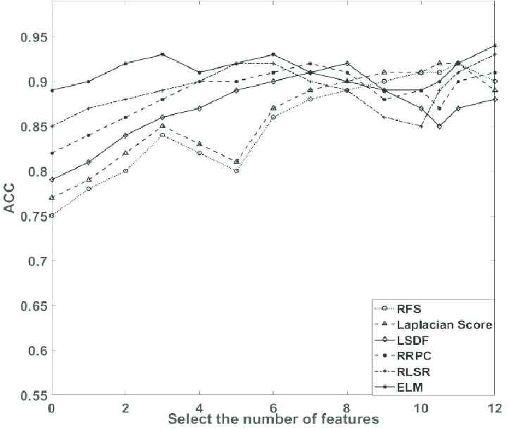
The NSL-KDD datasets are analyzed under different training sets and test sets to obtain the optimal training model parameters. Each feature selection algorithm is used to select the corresponding sample features in the training set. Then, the test sample is predicted by a SVM. The Acc of the predicted sample is calculated to obtain the corresponding experimental classification results. Five comparison algorithms are selected in this experiment, namely, the efficient robust feature selection algorithm (RFS) [36], Laplacian score [37], locally sensitive semi supervised feature selection (LSDF) [38], correlation and redundancy standard semi supervised feature selection (RRPC) [39], and semisupervised feature selection algorithm (RLSR) for readjusting linear regression [40]. Due to the random selection of the samples, classification accuracy may be unstable. Therefore, each experiment is conducted 20 times to obtain experimental results with high reliability, and the average value is used as the comparison result. The comparison diagrams of the accuracy of training set 75%+ test set 25% is given in Figure 8.
It is observed from Figure 8 the proposed feature selection algorithm is superior to the compared algorithm. Meanwhile, when 75% of the training set and 25% of the test set are combined, the accuracy of each method is better. Furthermore, the classification accuracy of the proposed method will also be improved with the increase in the number of selected features, verifying the effectiveness of the method.
Combination of different test sets and training sets.
4.4. Data Training Analysis
To verify the influence of different input samples and training on GAN training, the training method of the standard GAN model is referenced to verify the influence of the training parameters on the abnormal traffic detection model. First,
The conclusions can be drawn from Figure 9 as follows: first, bigger samples is not always better. Because when the input sample grows gradually, machine learning is difficult to extract useful features effectively in a large dataset. When the input sample is too small, the extracted features will be insufficient because of the poor generalization of the sample. Thus, the detection accuracy is low and the loss rate of the model in training is high. Second, when the training conditions under different input samples are compared, we can see that when the input samples are 3000 and the overall number of training epochs are set to 50, the training loss rate of the model reaches the minimum at 41 epochs. Thirdly, we also compare the loss rate of test values and verification values under different input samples as a comparison, and the conclusions are consistent with the foregoing. Therefore, the input samples of training are set as 3000 in this paper based on the above analysis. The overall number of training epochs are set 50. In this case, the loss rate of GAN model training is the lowest and the output effect of training is the best.
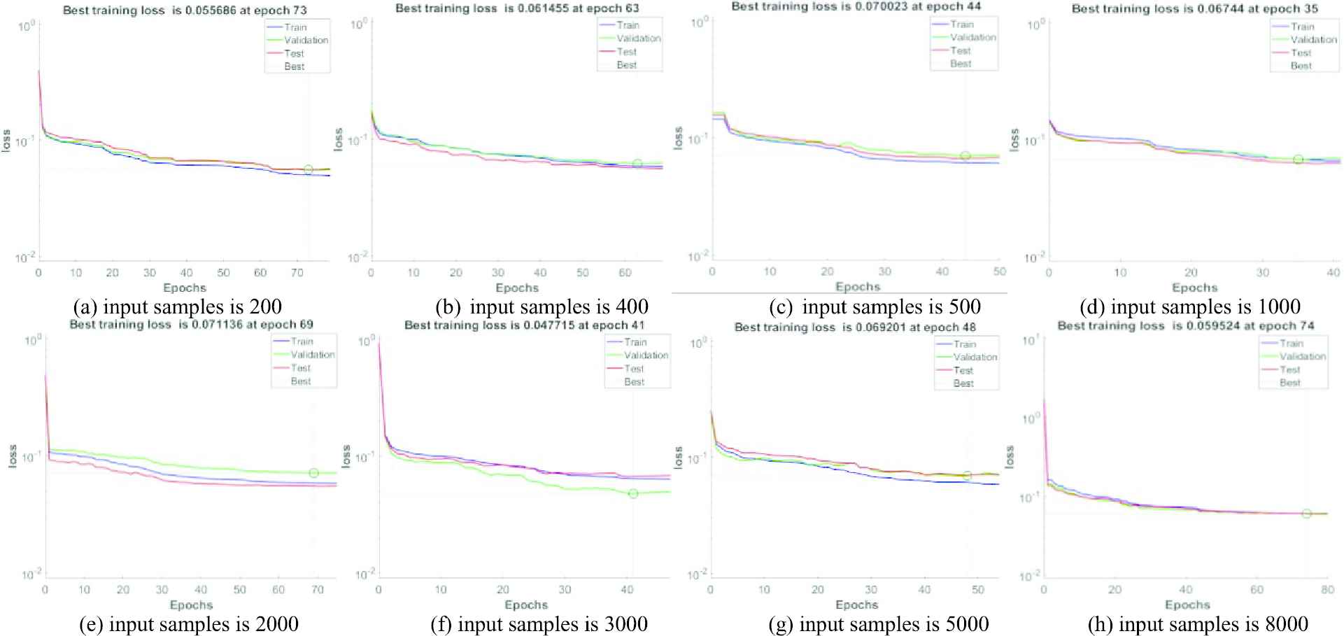
Comparison of data training analysis.
4.5. MK-MMD Performance Analysis Verification
Some of the data in the NSL-KDD datasets are used for training under different operating methods to verify the necessity of the MK-MMD optimization method. The sample mean distance and data loss rates in the training process are mainly compared in the experiment. The four methods are DBN, LSTM, GAN and the training method optimized using MK-MMD based on GAN. The comparison charts of the loss rates are shown in Figure 10a–10d.
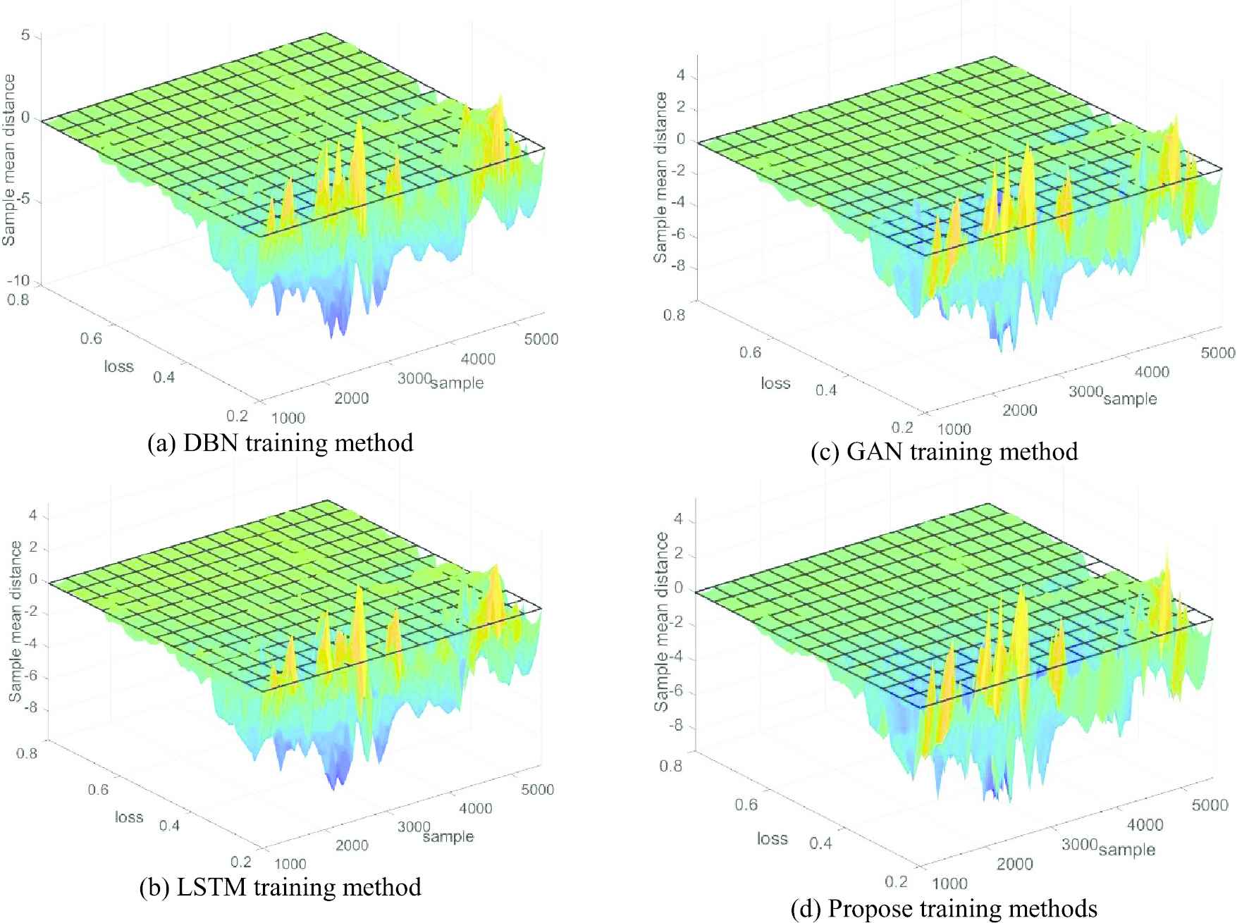
Comparison of the loss rates of the four methods.
The data loss rate of the NSL-KDD dataset under the DBN training method is shown in Figure 10a. It is observed from the figure that the dataset trained by the DBN method increases with the number of samples, and the data loss rate shows a decreasing trend. When the dataset number of samples increase to 3000, the mean distances between samples are the largest, and the loss rate is approximately 0.35. After the number of samples continue to increase, the mean distance becomes smaller, and the loss rate further increases. When the number of samples are 5000, the loss rate is approximately 0.5. The sample mean distance is reduced, causing the dataset to be misjudged by the training method. The obtained training effect is not ideal.
The comparison of the loss rate of the training dataset of the LSTM method is shown in Figure 10b. It is observed from the figure that the loss rate of the dataset after LSTM training is lower than that of the former. Meanwhile, the number of samples continue to increase, and the loss rate also shows a decreasing trend. The increase in the sample value has a strong influence on the sample mean distance. The dataset will also be misjudged during the training process.
The GAN method training dataset is shown in Figure 10c. It is observed from the figure that the dataset after GAN training has an average loss rate of approximately 0.3–0.4, which is lower than those of the previous two methods. The loss rate shows a decreasing trend due to the increasing number of samples. When the samples increase to 5000, the loss rate increases again. The misjudgment occurs during the data training process.
The final training dataset method proposed is shown in Figure 10d. It is clearly observed from the figure that the existing loss rate can be reduced to a small amount by the proposed method. The loss rate decreases with increasing number of samples, and the sample mean distance has little influence on the loss rate. The misjudgment and data loss rate can be reduced to a certain extent by the proposed method, verifying the necessity of this method.
4.6. Comparative Experimental Analysis of Classification Results
4.6.1. Two-classification performance comparison
The four types of abnormal traffics in the preprocessed NSL-KDD datasets are combined as an attack. The normal traffic is denoted as normal to verify the two-classification performance of the proposed method. A part of the datasets are selected for the verification analysis of the overall detection performance. The datasets are trained by four representative methods (DBN, LSTM and GAN) and the proposed method. (ROC) receiver operating characteristic curves (red curve represents normal traffic, black represents attack traffic) are drawn in Figure 11a–11d.
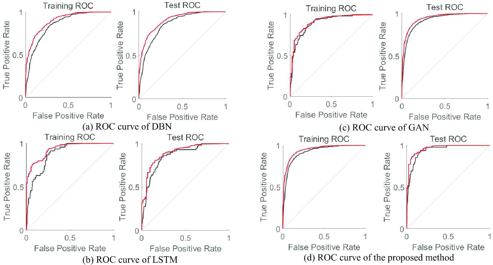
ROC curve comparison under different training methods.
It is observed from Figure 11a that when the DBN method is used to train the datasets, the obtained training ROC curve deviates strongly from the test ROC curve. The average AUC value (higher value corresponds to better performance) obtained by normal and attack traffic is approximately 0.78.
It is observed from Figure 11b that when the LSTM method is used to train the datasets, the AUC value of the training ROC curve is low, and the average value is approximately 0.64. Although the obtained AUC value of the test ROC curve is better, it deviates greatly from the training ROC curve. Therefore, the reliability is average, and the training effect is not good.
It is observed from Figure 11c that although the AUC value of the test ROC curve is better after being trained by the GAN method, it is approximately 0.85. However, the AUC value obtained by training the ROC curve is smaller, and is only 0.71. Therefore, the small training sample leads to an excessive training loss rate. The poor classification effect is verified when the dataset is trained using the GAN method.
It is observed from Figure 11d that when the proposed method is used to train data, both the ROC curve of training and the ROC curve of testing obtained a relatively high AUC value. The AUC value of the proposed method is better for both normal and attack traffic, highlighting the superiority of the proposed method.
The experimental comparison of Acc, recall rate, FPR, F-measure and AUC value for evaluating the two-classification is given in Table 6. The calculation of the parameters refers to Ref. [29].
| Method | Classification | Accuracy (%) | Recall (%) | FPR (%) | F-measure (%) | AUC |
|---|---|---|---|---|---|---|
| KNN | Normal | 42.739 | 59.356 | 41.297 | 49.695 | 0.581 |
| Attack | 56.384 | 68.418 | 35.984 | 61.821 | 0.657 | |
| DT | Normal | 76.612 | 79.634 | 15.936 | 78.094 | 0.708 |
| Attack | 81.278 | 82.347 | 9.307 | 81.810 | 0.708 | |
| SVM | Normal | 68.646 | 78.126 | 20.672 | 73.080 | 0.736 |
| Attack | 79.230 | 86.636 | 13.475 | 82.768 | 0.820 | |
| CNN | Normal | 75.839 | 83.724 | 15.266 | 79.587 | 0.814 |
| Attack | 83.257 | 87.341 | 5.215 | 85.250 | 0.869 | |
| RNN | Normal | 73.277 | 86.928 | 16.338 | 79.521 | 0.793 |
| Attack | 84.312 | 88.364 | 6.855 | 86.290 | 0.835 | |
| DBN | Normal | 81.541 | 86.466 | 8.419 | 83.931 | 0.862 |
| Attack | 87.158 | 91.107 | 3.217 | 89.089 | 0.837 | |
| LSTM | Normal | 83.503 | 88.832 | 7.309 | 86.085 | 0.848 |
| Attack | 90.227 | 93.527 | 1.484 | 91.847 | 0.879 | |
| GAN | Normal | 85.309 | 91.426 | 5.671 | 88.262 | 0.867 |
| Attack | 89.418 | 91.259 | 1.357 | 90.329 | 0.873 | |
| Proposed | Normal | 89.910 | 94.675 | 1.983 | 92.231 | 0.898 |
| Attack | 93.616 | 95.832 | 0.894 | 94.711 | 0.915 |
AUC, area under curve; CNN, convolutional neural network; DBN, deep belief network; D, decision tree; FPR, false positive rate; GAN, generative adversarial networks; KNN, K nearest neighbor algorithm; LSTM, long short-term memory; RNN, recurrent neural network; SVM, support vector machine.
Comparison of two-classification performance parameters.
It is observed from Table 6 that the performance of the proposed detection method is far superior to KNN, DT and SVM with regard to the test accuracy. These detection methods are traditional machine learning methods that show poor processing effectiveness on network traffic features. The normal and attack traffic in the network cannot be correctly classified. The detection accuracy of CNN, RNN, DBN, LSTM and GAN obtained by the five deep learning methods are higher than that of the abovementioned methods. But the detection accuracy of normal traffic is lower. The Accs for CNN, RNN, DBN, LSTM and GAN are 75.839%, 73.277%, 81.541%, 83.503% and 85.309%, respectively. All of these show lower accuracy than the proposed detection model. The Acc of the proposed method is 91.763% on average, demonstrating higher Acc is higher and improved performance is better. The three machine learning classification methods have low recall rates and poor classification performance in the comparison of recall rates. The recall rates of several detection methods based on deep learning are basically above 84%. The recall rate of the proposed method is 95.254% on average, which is the highest value compared to other methods.
The FPRs obtained by each method when detecting attack traffic are lower than the FPR of normal traffic in the comparison of FPR. The test set is composed of randomly selected datasets. Attack traffic has a larger proportion than normal traffic that is easier to detect. The FPR obtained by the proposed method is the lowest compared with other detection methods. The average FPR is 1.439%, which is far lower than those of the three traditional machine learning methods. Moreover, the average FPR of our method is also 8.802% lower than that of CNN, 10.408% lower than that of RNN, 4.379% lower than that of DBN, 2.958% lower than that of LSTM and 2.139% lower than that of GAN. Because the collaborative learning automatic is used to perform feature selection on network traffic. Moreover, the MK-MMD optimization method is used to continue to optimize the GAN. Therefore, the GAN with MK-MMD method has the lowest overall FPR.
The values obtained by several traditional machine learning methods are generally comparable to the harmonic average F-measure. The KNN method shows the worst performance with an average value of only 55.758%. The F-measure value obtained by the proposed method is the best among the five deep learning methods, and the average value is 93.471%. They are 11.055% and 10.565% higher than the corresponding values for the CNN and RNN methods. Moreover, they are 6.69% and 4.505% higher than the corresponding values for the DBN and LSTM methods.
It is observed from Table 6 that the AUC value of the proposed method is better regardless of whether normal or attack traffic is detected. The appropriate number of training epochs are selected during the training process, and the data loss rate is small.
The conclusions can be drawn by comparing and analyzing several types of parameter indicators: the proposed method has better performance on the two-classification task. The overall performance superiority of the proposed method in the detection of abnormal network traffics have also been verified.
4.6.2. Classification visualization
To compare the classification effect more intuitively, we set up a classification visualization experiment in this section for the 6 deep learning method. The specific classifications are shown in Figure 12a–12f.
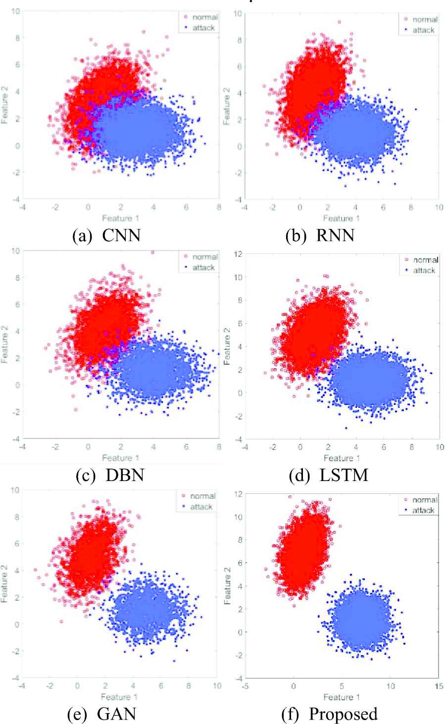
Visual comparison of classification.
The conclusions can be drawn from the figure: when CNN method is added (Figure 12a), the normal and attack traffic are disordered and discrete. The normal and attack traffic of the datasets cannot be effectively classified. When RNN method (Figure 12b) is used for training, the effect is improved to a certain extent compared with that mentioned above. But normal and attack traffic still failed to get effective separation. When the DBN method (Figure 12c) is added, it can be intuitively seen that the classification of normal and attack traffic have achieved good results. However, there is a certain degree of diffusion in the sample, so the effect is still poor. When the LSTM (Figure 12d) is added, the diffusion defects of the sample have been alleviated to some extent. The classification effects of normal and attack traffic are relatively good. However, the effective classifications of normal and attack are still not completed. Furthermore, after GAN (Figure 12e) is added, normal and attack traffic are effectively classified. However, the samples are mixed, and the convergence effects of the sample are poor. When the proposed method (Figure 12f) is added, normal and attack traffic have been fully classified, and the sample convergence effect is good. The effectiveness of each of the proposed strategies are further validated by this visualization experiment.
4.6.3. Multiclassification performance comparison
The performance of the proposed method cannot be fully explained if only the two-classification. Therefore, multiclassification performance of the proposed method is verified by experiments. The normal, probe, DoS, R2L and U2R in the NSL-KDD dataset are grouped into one category for the verification of multiclassification task. Therefore, ROC curve comparison graphs of the training ROC curve and the test ROC curve of normal traffic and four types of attack traffics are first presented. The AUC values of normal traffic and each type of attack traffic are mainly compared. The comparison results are shown in Figure 13a–13d.
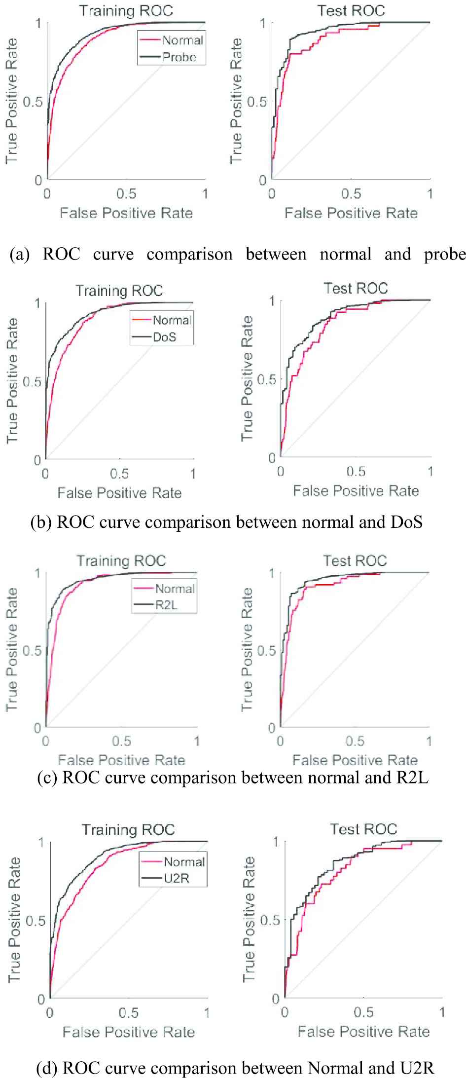
ROC curves comparison of data training.
The experimental comparisons of theAcc, recall rate, FPR, F-measure and AUC value of the five traffic types are given in Tables 7–11.
| Method | Accuracy (%) | Recall (%) | FPR (%) | F–measure (%) | AUC |
|---|---|---|---|---|---|
| KNN | 77.312 | 63.107 | 17.691 | 69.491 | 0.806 |
| DT | 73.487 | 71.265 | 21.636 | 72.359 | 0.793 |
| SVM | 79.251 | 69.378 | 17.329 | 73.987 | 0.824 |
| CNN | 82.346 | 79.149 | 15.647 | 80.716 | 0.887 |
| RNN | 85.628 | 82.573 | 8.264 | 84.073 | 0.893 |
| DBN | 87.369 | 84.184 | 4.179 | 85.747 | 0.917 |
| LSTM | 89.274 | 86.191 | 2.691 | 87.705 | 0.934 |
| GAN | 90.236 | 88.524 | 2.016 | 89.372 | 0.939 |
| proposed | 93.670 | 92.208 | 1.018 | 92.933 | 0.958 |
CNN, convolutional neural network; DBN, deep belief network; FPR, false positive rate; GAN, generative adversarial networks; KNN, K nearest neighbor algorithm; RNN, recurrent neural network; SVM, support vector machine.
Performance evaluation indexes of each algorithm on normal.
| Method | Accuracy (%) | Recall (%) | FPR (%) | F–measure (%) | AUC |
|---|---|---|---|---|---|
| KNN | 82.368 | 56.267 | 10.386 | 66.860 | 0.822 |
| DT | 62.603 | 59.705 | 15.587 | 61.120 | 0.751 |
| SVM | 73.478 | 71.423 | 13.276 | 72.436 | 0.793 |
| CNN | 79.247 | 82.217 | 9.361 | 80.705 | 0.804 |
| RNN | 84.424 | 88.562 | 5.143 | 86.444 | 0.887 |
| DBN | 88.585 | 91.783 | 3.287 | 90.156 | 0.929 |
| LSTM | 89.636 | 92.345 | 3.092 | 90.970 | 0.941 |
| GAN | 90.419 | 92.053 | 3.251 | 91.229 | 0.932 |
| proposed | 92.670 | 93.882 | 2.145 | 93.272 | 0.949 |
CNN, convolutional neural network; DBN, deep belief network; FPR, false positive rate; GAN, generative adversarial networks; KNN, K nearest neighbor algorithm; RNN, recurrent neural network; SVM, support vector machine.
Performance evaluation indexes of each algorithm on probe.
| Method | Accuracy (%) | Recall (%) | FPR (%) | F–measure (%) | AUC |
|---|---|---|---|---|---|
| KNN | 86.168 | 76.131 | 8.413 | 80.839 | 0.874 |
| DT | 79.213 | 81.395 | 11.348 | 80.289 | 0.817 |
| SVM | 84.711 | 78.754 | 9.667 | 81.624 | 0.863 |
| CNN | 88.732 | 69.217 | 6.258 | 77.769 | 0.891 |
| RNN | 91.424 | 71.138 | 4.296 | 80.015 | 0.938 |
| DBN | 92.313 | 87.342 | 4.022 | 89.759 | 0.942 |
| LSTM | 93.786 | 91.680 | 3.318 | 92.721 | 0.946 |
| GAN | 91.075 | 90.233 | 3.654 | 90.652 | 0.933 |
| proposed | 92.317 | 92.215 | 3.183 | 92.266 | 0.957 |
CNN, convolutional neural network; DBN, deep belief network; FPR, false positive rate; GAN, generative adversarial networks; KNN, K nearest neighbor algorithm; RNN, recurrent neural network; SVM, support vector machine.
Performance evaluation index of each algorithm on DoS.
| Method | Accuracy (%) | Recall (%) | FPR (%) | F–measure (%) | AUC |
|---|---|---|---|---|---|
| KNN | 82.176 | 68.313 | 12.741 | 74.606 | 0.867 |
| DT | 72.739 | 74.691 | 20.159 | 73.702 | 0.754 |
| SVM | 0 | 0 | Nan | Nan | 0 |
| CNN | 81.237 | 83.694 | 13.315 | 82.447 | 0.831 |
| RNN | 83.528 | 82.072 | 10.297 | 82.794 | 0.857 |
| DBN | 83.103 | 85.128 | 11.203 | 84.103 | 0.843 |
| LSTM | 85.312 | 87.254 | 8.413 | 86.672 | 0.872 |
| GAN | 86.937 | 89.208 | 6.109 | 88.058 | 0.893 |
| proposed | 89.634 | 91.362 | 4.510 | 90.489 | 0.928 |
CNN, convolutional neural network; DBN, deep belief network; FPR, false positive rate; GAN, generative adversarial networks; KNN, K nearest neighbor algorithm; RNN, recurrent neural network; SVM, support vector machine.
Performance evaluation index of each algorithm on R2L.
| Method | Accuracy (%) | Recall (%) | FPR (%) | F–measure (%) | AUC |
|---|---|---|---|---|---|
| KNN | 88.834 | 95.418 | 9.308 | 92.008 | 0.908 |
| DT | 67.103 | 75.672 | 19.294 | 71.130 | 0.717 |
| SVM | 38.246 | 33.617 | 57.452 | 35.782 | 0.401 |
| CNN | 65.236 | 88.105 | 20.419 | 74.965 | 0.738 |
| RNN | 76.375 | 90.373 | 14.743 | 82.786 | 0.802 |
| DBN | 80.128 | 92.536 | 8.208 | 85.886 | 0.849 |
| LSTM | 83.176 | 93.407 | 6.414 | 87.995 | 0.886 |
| GAN | 85.341 | 92.872 | 5.963 | 88.947 | 0.892 |
| proposed | 89.107 | 93.854 | 5.301 | 91.419 | 0.904 |
CNN, convolutional neural network; DBN, deep belief network; FPR, false positive rate; GAN, generative adversarial networks; KNN, K nearest neighbor algorithm; RNN, recurrent neural network; SVM, support vector machine.
Performance evaluation indexes of each algorithm on U2R.
An examination of the data presented in Table 7 shows that the parameter values obtained by the three machine learning methods are all lower for the normal traffic. The average Acc is 76.383%, and the average recall rate is 67.917%. The average F-measure value is 71.946%, and the average AUC value is 0.808, which are lower than those of the five deep learning methods. The FPR is as high as 18.886% on average, which is higher than that of the five deep learning methods. Therefore, the classification effects of the three traditional machine learning methods are general. The classification performance of the proposed method is the best among the five deep learning methods. The parameter values are the best, and the performance is improved. Meanwhile, the ROC curve comparison between normal and different attack traffic presented in Figures 13a–13d) show that the AUC value of the normal traffic is good, which is significantly different from the other attack traffics. Therefore, the classification effect of the normal traffic is better.
It is observed from Tables 8 and 9 that the DT method has the worst performance among the three traditional machine learning methods for probe traffic and DoS traffic. The Acc of probe traffic is only 62.603%, and the FPR is as high as 15.587%. The DoS Acc is only 79.213%, and the FPR is 11.348%. The DT method has poor feature extraction performance for probe. Moreover, the classification is overfitted due to the continuous overlapping classification of the DT method, and the performance is poor. The other two methods have a higher FPR than the deep learning method, even though they have a higher Acc. Therefore, the robustness is not strong, and the universality of classification is also poor.
The Accs of CNN, RNN, DBN and LSTM are all lower than 90% for probe traffic detection in the deep learning detection method. The Acc of the CNN method is only 79.247%, which is lower than that of the traditional KNN method. This is due to the translation invariance of the CNN method and improper parameter setting of the pooling layer. The average Acc of the remaining three methods are 87.548%, which is 5.122% lower than that of the proposed method. Meanwhile, the parameters obtained by the proposed method are also optimal. Although the accuracy of the LSTM method is higher than that of the proposed method in the detection of DoS traffic, the difference is only 1.469%.
The recall rate and AUC value of the proposed method (the ROC curve comparison result in Figure 13b) are both optimal. The proposed method have lowest FPR that is 3.075% lower than that of the CNN method, 1.113% lower than that of the RNN method, 0.839% lower than that of the DBN method, 0.315% lower than that of the LSTM method, and 0.471% lower than that of the GAN. Therefore, the proposed method has the best classification effect on probe traffic and DoS traffic based on the comparison of various parameters and the ROC curve.
It is observed from Table 10 that the Acc of KNN is higher than that of traditional machine learning methods for the detection of R2L traffic. However, the recall rate is lower, and is only 68.313%. The FPR is as high as 12.741%. All of the parameter values of the DT method are poor. The Acc is only 72.739%, and the FPR is as high as 20.159%, which is caused by the defects of the aforementioned DT itself. The Acc, recall rate, and AUC values are all 0. It is observed that the R2L traffic cannot be correctly identified in the SVM method. There are only a small number of R2L traffics are disguised as legitimate user identities. Their features are similar to those of normal packets. Meanwhile, the SVM algorithm is designed for the two-classification task. The training samples of multiclassification and high-dimensionality problems are badly processed, and the classification effects are also poor. The detection Accs of the five deep learning methods are higher than that of the above methods, but the FPRs are higher.
The FPRs of the CNN, RNN, DBN, LSTM and GAN methods are 13.315%, 10.297%, 11.203%, 8.413% and 6.109%, respectively. Therefore, the universality is general, and the robustness is poor. The performance of the proposed method is better than that of other methods, and the accuracy is improved to some extent. The ROC curve is similar to the training curve (Figure 13c), in which a better classification effect and superior performance are shown for the R2L attack types.
It is observed from Table 11 that the KNN method has the best effect on the detection of U2R traffic. The Acc is 88.834%. The recall rate is as high as 95.418%, and the AUC value is 0.908, indicating good results. The limited neighboring samples are used by the KNN method instead of using the class domain method to determine the category. Therefore, the classification performance of the KNN method is superior for the sample set to be classified with more cross or overlap of class domains. However, the KNN method requires a large amount of computation, especially when the number of features are very large, and the FPR is as high as 9.308%. So that its robustness is relatively weak. The Accs of the DT and SVM methods are only 67.103% and 38.246%, respectively, and the recall rates are 75.672% and 33.617%, respectively. The reasons for poor performance are consistent with the data types described above. The CNN method displays the worst performance among the five deep learning methods, with an Acc of only 65.236%. The accuracy of CNN is lower than that of the KNN method and DT method. The reasons for the poor performance are also consistent with the above mentioned results. The Acc obtained by RNN, DBN and LSTM is 79.893% on average, which is 9.214% lower than that of the proposed method.
Although the recall rate is similar to the proposed method, the FPR is much lower than the three methods. The AUC value is also the best in the proposed method. The reason is that collaborative LA are adopted to optimize the selection of features of the NSL-KDD dataset. The gap between the numbers of different data types can be reduced to a certain extent. More U2R features are learned by the model, improving the classification effect.
The performance indexes obtained by the proposed detection model for normal and four kinds of attack are all better as observed from the performance parameters presented in Tables 7–11. Some parameters are lower than other methods. However, both the detection performance and classification effect of the proposed method are the best based on the overall comparison, and can effectively classify the NSL-KDD dataset. Thus, the effectiveness and superiority of the multiclassification task are verified for the proposed method.
4.6.4. Method stability verification
The comparison of the classification FPRs of CNN, RNN, DBN, LSTM, GAN and the proposed method are experimentally verified when the datasets are mixed with other sample values of 200, 500, 1000 and 2000. The stability of the proposed algorithm on the dataset is analyzed for verification in Table 12.
| Method | FPR (%) | |||
|---|---|---|---|---|
| Mix into Samples 200 | Mix into Samples 500 | Mix into Samples 1000 | Mix into Samples 2000 | |
| CNN | 2.354 | 4.105 | 6.347 | 10.298 |
| RNN | 1.871 | 2.672 | 4.293 | 7.246 |
| DBN | 3.583 | 5.945 | 7.567 | 9.352 |
| LSTM | 1.291 | 1.964 | 2.483 | 3.617 |
| GAN | 1.264 | 1.757 | 2.096 | 3.118 |
| proposed | 0.837 | 0.891 | 1.108 | 1.412 |
CNN, convolutional neural network; DBN, deep belief network; FPR, false positive rate; GAN, generative adversarial networks; RNN, recurrent neural network.
Comparison of false positives rate under different mixed samples.
It is observed from the Table 12 that when the mixed samples are 200, the DBN abnormal detection model has the highest FPR that is equal to 3.583%. However, the lowest FPR of the proposed method is 0.837%. When the mixed samples are continuously increased, the FPR of CNN and DBN increases greatly. When the mixed samples are increased to 2000, the FPRs of CNN and DBN are 10.298% and 9.352%, respectively. Therefore, the classification effect and the stability of the method are the worst. These two methods are most affected by the mixed sample. The FPR of the proposed method is 1.412% for the mixed sample size of 2000.
The proposed method has lowest FPR value compared with other methods, and the classification results obtained are better. When the mixed samples are continuously increased, the FPRs of the other five methods increase greatly based on the horizontal comparison. On the other hand, the FPR of the proposed method increases monotonically with increasing samples size. However, the amplitudes are not large, and the stability is verified.
5. CONCLUSIONS
An algorithm for generating countermeasure network and feature optimization selection for abnormal traffic detection is proposed in this paper. The network dataset NSL-KDD has been used for experimental analysis to improve the problem of poor parameters such as Acc, recall rate, FPR and AUC in the existing methods. The main conclusions are as follows:
The optimal feature subset is obtained through feature optimization selection of traffic by collaborative learning automatic. The influence of useless features in data samples are reduced on classification accuracy.
GAN network is used to analyze the samples, and appropriate generators and classifiers are designed to complete the sample training. The MK-MMD is used to minimize the interdomain distance and better assist the multiclassification model detection of abnormal traffic. The detection accuracy is further improved,
The detection results are output through the 16-dimension Softmax classifier. The necessity of each step of the proposed method is verified by setting various comparative experiments. It is concluded from the experiment that the proposed method has the best effect on various evaluation indexes in the verification of the overall performance and individual performance. It has obvious advantages and the robustness is the strongest compared with other methods.
CONFLICTS OF INTEREST
The authors declare no conflict of interset.
AUTHORS' CONTRIBUTION
All authors contributed to the work. All authors read and approved the the manuscript.
ACKNOWLEDGMENTS
The authors express great thanks to the financial support from the National Natural Science Foundation of China.
This research was funded by the National Natural Science Foundation of China, grant number 61703349; the Fundamental Research Funds for the Central Universities, grant number 2682017CX101, 2682017ZDPY10 and the Key Research Projects of the China Railway Corporation, grant number 2017X007–D.
REFERENCES
Cite this article
TY  - JOUR
AU  - Wengang Ma
AU  - Yadong Zhang
AU  - Jin Guo
AU  - Kehong Li
PY  - 2021
DA  - 2021/03/19
TI  - Abnormal Traffic Detection Based on Generative Adversarial Network and Feature Optimization Selection
JO  - International Journal of Computational Intelligence Systems
SP  - 1170
EP  - 1188
VL  - 14
IS  - 1
SN  - 1875-6883
UR  - https://doi.org/10.2991/ijcis.d.210301.003
DO  - 10.2991/ijcis.d.210301.003
ID  - Ma2021
ER  -