
Deep Encoder–Decoder Neural Networks for Retinal Blood Vessels Dense Prediction
 , Bo Fu1, Mehrdad Aliasgari1
- DOI
- 10.2991/ijcis.d.210308.001How to use a DOI?
- Keywords
- Deep learning; Encoder-decoder; Retinal blood vessel; Dense prediction
- Abstract
Automatic segmentation of retinal blood vessels from fundus images is of great importance in assessing the condition of vascular network in human eyes. The task is primary challenging due to the low contrast of images, the variety of vessels and potential pathology. Previous studies have proposed shallow machine learning based methods to tackle the problem. However, these methods require specific domain knowledge, and the efficiency and robustness of these methods are not satisfactory for medical diagnosis. In recent years, deep learning models have made great progress in various segmentation tasks. In particular, Fully Convolutional Network and U-net have achieved promising results in end-to-end dense prediction tasks. In this study, we propose a novel encoder-decoder architecture based on the vanilla U-net architecture for retinal blood vessels segmentation. The proposed deep learning architecture integrates hybrid dilation convolutions and pixel transposed convolutions in the encoder-decoder model. Such design enables global dense feature extraction and resolves the common “gridding” and “checkerboard” issues in the regular U-net. Furthermore, the proposed network can be efficiently and directly implemented for any semantic segmentation applications. We evaluate the proposed network on two retinal blood vessels data sets. The experimental results show that our proposed model outperforms the baseline U-net model.
- Copyright
- © 2021 The Authors. Published by Atlantis Press B.V.
- Open Access
- This is an open access article distributed under the CC BY-NC 4.0 license (http://creativecommons.org/licenses/by-nc/4.0/).
1. INTRODUCTION
Human eyes are sensitive to vascular system pathologies. A variety of diseases such as diabetic retinopathy, cardiovascular disease and stroke can cause a malfunction of blood vessels in the retina, which can severely impair human vision. According to American Diabetes Association, diabetes is currently the most common cause of blindness in the western world.
Manual vessel segmentation from retinal fundus images is a tedious and time–consuming task, which requires experience and relevant domain knowledge. Therefore, automatic segmentation of retinal blood vessels is a highly demanding technique, and yet it is a challenging task due to the low contrast of images, the variety of vessels and potential pathology. Retinal blood vessels in different local regions vary hugely in size and shape, e.g., the width of the retinal vessels can range from 1 pixel to 20 pixels. In the presence of potential retinal diseases, the vessels can exhibit quite different patterns and features. The variety of retinal blood vessels make it difficult to use artificially designed features to perform the detection and segmentation.
A number of methods have been proposed for retinal vessels segmentation. Most of these methods utilized shallow machine learning algorithms to extract local features including support vector machine [36], decision tree [9], multi–scale Gabor Filters [13], and model based tracing [14], etc. However, these methods require specific domain knowledge, and the efficiency and robustness of these methods are not satisfactory for medical diagnosis. In recent years, deep learning models, such as Fully Convolutional Networks [34,56,31], U–net [40], Deeplab [5], and SegNet [3], have made great progress in various image segmentation tasks. There are several recent studies that utilized well–known CNN models such as VGGnet, Googlenet, and U–net for retinal blood vessels segmentation [30,28,15,19,18,10]. However, these models are incapable of detecting tiny edges and contours in the low contrast retinal blood vessel images due to spatial and local information loss caused by normal convolutions and pool operations. Also, they heavily rely on the postprocessing procedure.
In this study, we propose a novel end–to–end deep learning network for retinal blood vessels segmentation. The proposed model is implemented on Digital Retinal Images for Vessel Extraction (DRIVE) and Structured Analysis of the Retina (STARE) retinal blood vessel data sets. The experimental results show that our proposed model outperforms the baseline U–net model. The proposed encoder–decoder network is built upon the U–net architecture. In the encoder path, hybrid dilation convolution (HDC) layers are implemented to prevent the loss of spatial information. Each hybrid convolution layer contains three consecutive dilation operations with different dilation rates that are carefully chosen to preserve the neighboring information. In the decoder path, the novel pixel transposed convolution layers are implemented to prevent the checkerboard problem raised from normal up–sampling layers. By implementing the HDC layers and pixel transposed convolution layers, the proposed model is able to capture subtle features such as tiny edges and contours which are essential for retinal blood vessels segmentation problem. Additionally, the proposed model can be effectively trained end–to–end to perform the dense prediction without relying on postprocessing procedure such as Conditional Random Field (CRF). Even though we only implement the proposed model on the retinal blood vessels image data sets, the model can be applied to a broader range of detention and segmentation tasks.
The remaining of the paper is organized as follows. In Section 2, we provide a overview of the related works about semantic segmentation and blood vessel detection. In Section 3, we present the two essential modules in detail and illustrate the overall framework design. Section 4 contains the experimental results and thorough discussion of the model performance.
2. RELATED WORK
The task of retinal blood vessels segmentation has been studied from different perspectives. Fraz et al. provided an extensive review [14]. In general, these methods fall into two categories: shallow machine learning based methods and deep learning based methods.
2.1. Shallow Machine Learning Based Methods
There are many studies that utilized shallow machine learning algorithms to extract local features including support vector machine, decision tree, multi–scale Gabor Filters, model based tracing, etc. These methods fall into two categories: unsupervised and supervised learning methods.
In unsupervised methods, blood vessel features such as color, shape, gradient, and contrast are used to construct templates to estimate a match at each pixel against the pixel's surrounding windows. The representatives of this category are matched filtering method and vessel tracking–based method. Matched filtering method introduces the expected appearance of vessels to distinguish vessel pixels from nonvessel pixels. The matched filters are implemented using 2–dimensional (2D) kernels that convolve a retinal image. Several models have been introduced to construct the matched filters. Chaudhuri et al. modeled the cross–section of a vessel by a Guassian shaped curve, and extended to 2D by assuming that a vessel has a fixed width and direction for a short length [4]. Pinz et al. used a standard gradient filter to detect pixels on the boundary of vessels [37]. Hoover et al. used both local and region–based vessel features cooperatively to segment the vessel network [21]. A recent study used a combination of shifted filter responses, COSFIRE filters, to extract vessels [2]. Even though matched filtering technique performs quite well on healthy images, it is prone to increasing the false positive rates with pathological images [14]. Tracking–based techniques use a profile model to track vessels at the starting points, such as the papilla in the retina. The tracking process stops when the response to the profile model falls below a given threshold, e.g., a fuzzy model of a one–dimensional (1D) vessel profile was utilized to track vessels [47]. Tracking–based techniques can provide highly accurate vessel widths, but is prone for termination at branch points, which are not well detected by 1D filters.
Supervised methods use extracted feature vectors and annotated images to train a classifier. Segmentation task is considered as a problem of pixel–level classification. Traditional shallow supervised learning methods, such as supporter vector machine, decision tree, and artificial neural network [32], have been proposed to segment the blood vessels. Feature extraction is a key step for these supervised learning methods. Fraz et al. utilized four techniques to extract features, including gradient vector field, morphological transformation, line features, and Gabor response. Marin et al. simultaneously integrated gray–level and moment invariant–based features to build the 7–D feature vectors to train artificial neural networks [32]. Nguyen et al. proposed a novel line detection based on the linear combinations of varying scales [33]. Supervised learning methods usually outperform the unsupervised learning methods. However, most of the existing supervised methods use artificially designed features to model retinal vessels. Such manual feature design is heavily dependent on domain knowledge [28]. In the presence of potential retinal diseases, the retinal vessels can exhibit different patterns and features, which makes the segmentation task even more challenging.
2.2. Deep Learning Based Methods for Dense Prediction
In the last decade, deep learning models, especially Convolutional Neural Networks (CNNs), have made spectacular progress in pattern recognition and computer vision tasks such as image recognition [23,26,59,29,43,46,25,20,52], semantic segmentation [34,31,40,57,58], instance segmentation [50], object detection [20,17,39], video generation [51] and data completion [27,44], etc. CNN models are typically used to analyze grid–structured images, and are able to capture the hierarchical features in the images. More importantly, CNN models can automatically extract features, thus no artificially designed features or prior knowledge are required. Recently, Fully Convolutional Networks (FCNs) [34,56,31] and U–net [40], have achieved promising results in dense prediction tasks. FCN models can produce the dense prediction output map from input of any arbitrary size, and alleviate the spatial information loss issue. The U–net architecture is built upon the FCN. The basic structure of the U–net consists of three core aspects: encoder, decoder, and skip connections. Input of the network is first contracted into an encoder bottleneck for feature extraction. The extracted features are then expanded to the original dimensions of the input through the decoder path using up–sampling. By combining the location information from the encoder path with the contextual information in the decoder path, the U–net is effective for dense prediction tasks. Deep learning models have been applied in various biological and medical imaging applications, such as neural segmentation in electron microscopy (EM) images [57,11], brain segmentation [27,58], lung segmentation [41], etc. However, for retinal blood vessel segmentation, there are only a few studies that utilized deep learning models. Liskowski and Krawiec was the first study that applied CNNs for retinal blood vessels segmentation [30]. Li et al. presented a cross–modality mapping function from color retinal image to vessel map [28]. Fu et al. proposed a multi–scale and multi–level CNN, which combined the CRF and a so–called side–output layer based on the idea of auxiliary classifiers in inception module [15]. However, these works heavily rely on either preprocessing or postprocessing to enhance the final results, and are not completely automatic. Dasgupta and Singh treated the retinal blood vessels as a multi–label problem, and used fully convolutional network to integrate the structural prediction method [12]. Alom et al. proposed a Recurrent Convolutional Neural Network (RCNN) and a Recurrent Residual Convolutional Neural Network (RRCNN) based on the U–net architecture. These two models were implemented on a number of segmentation applications such as blood vessel, skin cancer and lung lesion segmentation tasks [1]. Two recent studies implemented the dilated spatial pyramid pooling block for optics disc, lungs, and retinal blood vessel segmentation tasks [19,18], however, they ignored the decoder path. Our proposed model also utilizes dilation blocks to preserve spatial information in the intermediate feature maps and prevent the gridding issue, but we specifically use hybrid dilation modules with different dilation rates. To make the dilation module more effective, we also improve the decoder path by adding pixel transposed convolutional layers (PixelTCL) to resolve the checkerboard issue.
3. THE PROPOSED DEEP LEARNING DENSE PREDICTION METHOD
In this section, we introduce the proposed deep encoder–decoder model. The proposed model combines the HDC layers and the pixel transposed convolution layers in the down–sampling and up–sampling path, respectively. By combining these modules, we can effectively eliminate the loss in the neighboring context (i.e., the gridding issue), generate high–resolution feature maps in the up–sampling and alleviate the checkerboard problem.
3.1. HDC Module
Dilated convolution (or Atrous convolution) is a key technique that has been extensively studied for semantic segmentation applications in recent years [5–6,7,53,49,54]. The objective of dilated convolutions is to expand the receptive field in order to preserve spatial and contextual information. The idea is to insert “holes” in the convolution kernel to increase the resolution and maintain the spatial information in the intermediate receptive fields. Yu and Koltun was the first study that stacked several dilation layers with increasing dilation rates to aggregate the multi–scale contextual information [53]. However, the area covered by the receptive field suffered from the “gridding” issue, and the model failed to capture the neighboring context. To illustrate this issue, supposing that the convolution kernel is 3 and the dilation rate is 2, then only 36% of the whole receptive field (i.e., 9 out of 25 pixels) is used for computation. This so-called “gridding” issue becomes more and more significant as the dilation rate increases in the higher layers which would affect the consistency of local information.
Wang et al. proposed a HDC framework to address the above problem [49]. The intuition is to eliminate the loss of maximum distance and utilize the full size of the receptive field without any missing holes. They implemented a series of dilation convolutions with different rates which do not have common divisors. As a result, the final receptive field is able to cover adequate pixels area and preserve neighboring context(i.e, no missing holes).
In this study, we adopt HDC framework in the encoder path for the following reasons. (1) Size of objects: retinal blood vessels varies hugely in size and shape. Some vessels are tiny (the width of a vessel can be as small as 1 pixel) and have subtle details. (2) Layout of objects: retinal blood vessels are densely distributed and connected, and the existence of vessel crossing, branching and center–lining makes the segmentation task even more challenging. Preserving both the context information and resolution of the image are crucial to segment such a tight crowd of small vessels. Dilation layers enable expanding the receptive field without losing resolutions. Additionally, by implementing two groups of three consecutive dilated convolution layers with different dilation rates, which are carefully chosen to avoid having a common factor relationship, we are able to eliminate the gridding issue and preserve neighboring information without sacrificing computational capability.
3.2. Pixel Transposed Convolution Module
Up–sampling layers play an important role in the decoder path for recovering the spatial feature maps. Many encoder–decoder architectures use transposed convolutional layers in the decoder path for up–sampling [55,56,31,38,48,22]. The transposed convolution can be considered as performing multiple independent convolutions on the input feature map followed by a periodical shuffling operation. Formally, given an input feature map
One critical limitation of the transposed convolution is the checkerboard problem [35]. Because the intermediate feature maps (i.e.,
Since retinal blood vessels are densely distributed and closely connected with each other, discontinuities among adjacent pixels caused by regular transposed convolutions may directly affect the accuracy of the segmentation. Therefore, the checkerboard problem is more detrimental for retinal blood vessels segmentation task. To mitigate the checkerboard problem, we adopted the simplified PixelTCL framework to up–sample from the low–resolution feature map to the high–resolution feature map, which enables direct connections among adjacent pixels on the final output feature map. Specifically, we generate four intermediate feature maps sequentially in each Up–sampling Block (UBs) of the encoder path. The first intermediate feature map depends on the input feature map. To avoid the redundant information of the input feature map, the second intermediate feature map only relies on the first intermediate feature map. Similarly, the third intermediate feature map is created based upon the first and second intermediate feature maps. The fourth intermediate feature map is created based upon the first, second, and third intermediate feature maps. Formally, an intermediate feature map
3.3. Framework Design
The existing dataset for retinal blood vessels segmentation have several limitations. First, the total number of fundus images is limited. The DRIVE dataset contains 40 images in total (20 for training and 20 for testing), and the STARE dataset contains only 20 images. Second, the available images have relatively low contrast. To overcome these challenges, we propose a framework that aims to achieve the following objectives: (1) The capability of classification in a multi–scale context. (2) The high efficiency regarding both of the training and testing computation cost. (3) The capability of not heavily replying on postprocessing methods.
Our proposed framework is illustrated in Figure 1. Even though we implement the proposed model for retinal blood vessels segmentation, the model can also be implemented for a broader range of detection and segmentation tasks. As illustrated in Figure 1, at each resolution level in the encoder path, we utilize the bottleneck network and the identify mapping function to reduce the complexity and resolve the gradient vanishing issue [20]. The encoder path contains four Down–sampling residual Blocks (DBs) in total. Within each block, there are two
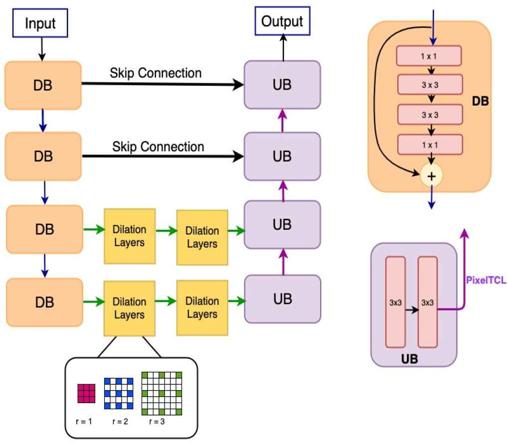
An illustration of framework design. In the Down–sampling residual Block (DB), 1 × 1 means 1 × 1 convolution and 3 × 3 means 3 × 3 convolution. Max-pooling operations are used to connect the DBs. Each Up–sampling Block (UB) has two 3 × 3 convolution. Pixel transposed convolutional layers (PixelTCL) is used to connect the UBs.
In the proposed model, we improve both the encoder and decoder by combing the HDC module and PixelTCL module. PixelTCL module is able to generate connections among adjacent pixels in the final output feature map and mitigate the checkerboard issues. The HDC module is able to preserve the spatial and local information and maintain the resolution as the encoder path goes deeper. More importantly, using HDC module in the encoder path can make PixelTCL module in the decoder path more effective since it can have large–scale information for computation.
4. EXPERIMENTAL STUDIES
The proposed model is implemented on two data sets: DRIVE [45] and STARE [21]. The DRIVE database was built by a diabetic retinopathy screen program to study the segmentation of retinal blood vessels in the Netherlands. This program contains 400 diabetic subjects with the age range of 25 to 90 years old. Out of these 400 diabetic subjects, 40 subjects were randomly selected for the segmentation study. Among these subjects, 7 subjects showed the mild signs of early diabetic retinopath, and the rest were normal. Each image is captured with a 3CCD camera and has a diameter of approximately 540 pixels. For each image, the result of manual segmentation of the vessel maps is provided for comparison purpose. Two examples of the data in DRIVE are provided in Figure 2.
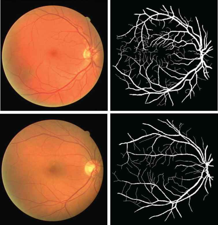
Two examples from Digital Retinal Images for Vessel Extraction (DRIVE) data set. The top row is the normal retinal image and the corresponding manual segmentation. The bottom row is the abnormal retinal image that has Background Diabetic Detinopathy, and the corresponding manual segmentation.
STARE2 contains 20 retinal fundus images for testing purpose [21]. Each image was taken by a TopCon TRV–50 fundus camera with a dimension of
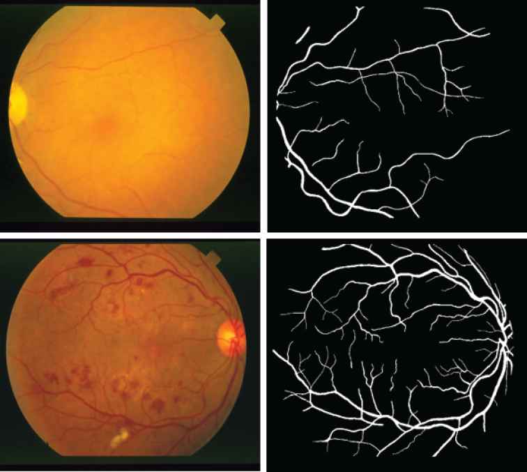
Two abnormal examples from Structured Analysis of the Retina (STARE) data set. The top row is Emboli, Nonhollenhorst and the corresponding manual segmentation. The bottom row is Background Diabetic Retinopathy and the corresponding manual segmentation.
4.1. Experimental Setup
We use the U–net model as our baseline. In addition, we explore three encoder–decoder architectures in which either the HDC module or Pixel Transposed Convolution module, and both are included. The three deep architectures are: (1) HDC with U–net; (2) Pixel Transposed Convolution with U–net; (3) The combination of HDC and Pixel Transposed Convolution in the down–sampling and up–sampling layers respectively. All the four above mentioned models are trained and tested on DRIVE and STARE data sets.
The data in DRIVE are split into training set and testing set, each containing 20 images from different subjects. Due to the limited number of images, we extract
For each CNN model, Rectified Linear Units (ReLUs) are used followed by the convolutional layers. Dropout is also included and set to 0.2. All models are trained with the ADAM [24] optimizer (rather than Stochastic Gradient Descent (SGD)). The hyperparameters are set as follows: Learning Rate = 0.01, Beta1 = 0.2, Beta2 = 0.999, Epsilon = 0.1, and Weight Decay = 0.001. The machine used for training has the following configurations: NVIDIA RTX 2080 Ti 11 GB GPU, Intel i7–7820X 8 Core 4.30GHz, and CentOS 7 operating system. We implement all the deep learning models using Tensor-Flow backend in Keras API. It took 3 hours in the offline training procedure and the inference took about 1 minute to process.
To evaluate the performance of different models, we use the area under ROC curve (AUC), accuracy (ACC), sensitivity (SE), and specificity (SP). The three measures are calculated as follows:
4.2. Experimental Results and Discussion
The performance of the four models on DRIVE data set is summarized in Table 1. Overall, all the three proposed models outperform the U–net baseline model. Especially, HDC + PixelTCL model achieves the best performance in the measurement of Accuracy and Specificity, while PixelTCL with U–net achieves the best performance in the measurements of AUC and Sensitivity. In this quantitative comparison, we can see that the performance of U–net on Drive data set is already fairly good. Nevertheless, HDC + PixelTCL module can still improve the performance by a small margin. Table 1 also shows that PixelTCL with U–net outperforms the HDC with U–net. Dilation layers have been used in previous studies, but less attention was paid to the up–sampling. In this experiment, we prove that by using PixelTCL in the up–sampling, it can effectively eliminate the checkerboard issue and preserve dependency among intermediate feature maps.
| Network | AUC | ACC | SE | SP |
|---|---|---|---|---|
| U-net | 0.9792 | 0.9560 | 0.7636 | 0.9821 |
| HDC with U-net | 0.9816 | 0.960 | 0.7701 | 0.9814 |
| PixelTCL with U-net | 0.9862 | 0.9657 | 0.7879 | 0.9855 |
| HDC + PixelTCL | 0.9829 | 0.9683 | 0.7842 | 0.9873 |
ACC, accuracy; AUC, area under ROC curve; DRIVE, Digital Retinal Images for Vessel Extraction; HDC, hybrid dilation convolution; PixelTCL, Pixel transposed convolutional layers; SE, sensitivity; SP, specificity.
Comparison of results on DRIVE.
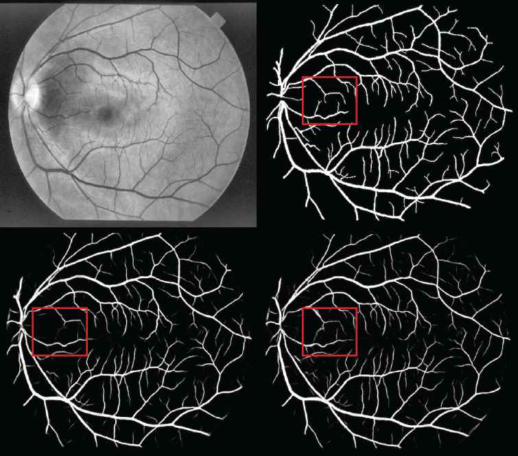
Figure 4 shows a visualization of the experimental results. The top left image is the preprocessed retinal image. The top right image shows the ground truth based on manual segmentation. The bottom left image shows the result of the U–net baseline model. The bottom right image shows the result of the proposed HDC + PixelTCL model. In general, the results of the proposed model is much closer to the ground truth than that of the U–net model. E.g., when comparing the red square region in both images, it clearly shows that the result of the U–net model contains a number of noises (i.e., wrong prediction), while the result of the proposed model is able to remove most of these noises and very similar to the ground truth (i.e., the number of False Positives is smaller in the proposed model). Furthermore, the proposed model is able to capture more of the tiny branch vessels than the U–net model (i.e., the number of True Positives is bigger in the proposed model).
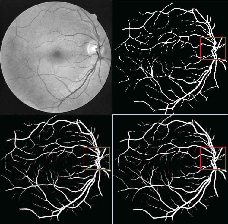
Digital Retinal Images for Vessel Extraction (DRIVE) performance.
Table 2 summarizes the performance of the four models on STARE database. HDC + PixelTCL model achieves the best performance in the measurements of AUC and Accuracy. PixelTCL with U–net has the highest Sensitivity, while the Sensitivity of HDC + PixelTCL model is the second highest with the difference of 0.0005. Although U–net model gets the highest Specificity, but the different between HDC + PixelTCL and U–net in Specificity is only 0.0013. Because STARE database only contains 20 images, small patches need to be extracted from each image to ensure enough number of training images. As a result, each input image has a very low resolution with
| Network | AUC | ACC | SE | SP |
|---|---|---|---|---|
| U-net | 0.9815 | 0.9536 | 0.8124 | 0.9831 |
| HDC with U-net | 0.9809 | 0.9572 | 0.8172 | 0.9789 |
| PixelTCL with U-net | 0.9793 | 0.9496 | 0.8214 | 0.9824 |
| HDC + PixelTCL | 0.9829 | 0.9614 | 0.8209 | 0.9818 |
ACC, accuracy; AUC, area under ROC curve; STARE, structured Analysis of the Retina; HDC, hybrid dilation convolution; PixelTCL, Pixel transposed convolutional layers; SE, sensitivity; SP, specificity.
Comparison of results on STARE.
A visualization of the segmentation results is given by Figure 5. The top left image is the preprocessed retinal image. The top right image shows the ground truth based on manual segmentation. The bottom left image shows the result of the U–net baseline model. The bottom right image shows the result of HDC + PixelTCL model. As showed in the figure, the performance of the proposed model is much better than the U–net model. In particular, for the red square region in both images, the U–net model fails to capture several tiny branches of retinal blood vessels, while the proposed model is able to detect more tiny branches and subtle details than the U–net model.
Structured Analysis of the Retina (STARE) performance.
5. CONCLUSION AND FUTURE WORK
In this study, we investigate the dense prediction task of retinal vessels segmentation. Even though a number of methods have been proposed for this task, most of these methods fail to preserve enough spatial and local information, thus suffering from gridding and checkerboard problems. To resolve the problems, we propose a novel deep learning neural network which builds upon the U–net architecture. In particular, we utilize HDC and Pixel Transposed Convolution in the encoder–decoder network. We implement the proposed models on two data sets: DRIVE and STARE. The quantitative results show that the proposed models outperform the U–net model. We also provide visualizations to demonstrate that our model is able to catch more subtle details and remove more noises than the baseline U–net. In the future, we plan to employ recurrent neural networks and nonlocal attention network to further improve the performance of dense prediction in retinal blood vessels and biomedical imaging tasks.
CONFLICTS OF INTEREST
The authors declare no conflicts of interest.
AUTHORS’ CONTRIBUTIONS
WZ conceived the project, LL and WZ designed the methodology, VC and WZ performed the experiments, BF and MA interpreted the results, WZ and LL drafted the manuscript. All authors have read and approved the final manuscript.
ACKNOWLEDGMENTS
Thanks for the great support of NVIDIA Corporation with the donation of the Tesla Titan Xp GPU.
Footnotes
REFERENCES
Cite this article
TY  - JOUR
AU  - Wenlu Zhang
AU  - Lusi Li
AU  - Vincent Cheong
AU  - Bo Fu
AU  - Mehrdad Aliasgari
PY  - 2021
DA  - 2021/03/22
TI  - Deep Encoder–Decoder Neural Networks for Retinal Blood Vessels Dense Prediction
JO  - International Journal of Computational Intelligence Systems
SP  - 1078
EP  - 1086
VL  - 14
IS  - 1
SN  - 1875-6883
UR  - https://doi.org/10.2991/ijcis.d.210308.001
DO  - 10.2991/ijcis.d.210308.001
ID  - Zhang2021
ER  -