
Modified 2-Way Wavefront (M2W) Algorithm for Efficient Path Planning
- DOI
- 10.2991/ijcis.d.210305.002How to use a DOI?
- Keywords
- Robotic path planning; Safe path generation; Wavefront algorithms; Self-organizing maps; Artificial potential fields; Navigational function; Glasius model
- Abstract
In this paper modified 2-way wavefront algorithm(M2W) is introduced for the discretized path planning problem. The proposed scheme uses the Glasius model, wavefront navigational function, and adaptation of Artificial Potential Fields (APF) for effective obstacle avoidance. Unlike the APF, it does not suffer from local minima, and it addresses the shortcoming of the navigational method by generating paths that are not “too close” to obstacles. Furthermore, compared to the Glasius model, M2W's computation time is significantly reduced, especially in a complex workspace with a higher density of obstacles. The proposed algorithm is also simulated with an additional set of planning constraints to demonstrate the adaptability of the M2W for constraint planning problems.
- Copyright
- © 2021 The Authors. Published by Atlantis Press B.V.
- Open Access
- This is an open access article distributed under the CC BY-NC 4.0 license (http://creativecommons.org/licenses/by-nc/4.0/).
1. INTRODUCTION
For the last six decades, with maturity in robotics and computers, numerous path planning methods have evolved addressing different needs and requirements. Each method has its strengths and weaknesses, with no one fix for all; the specific system requirements mostly dictate the choice of planning methods. Existing work for robot path planning can be divided into two broad categories: (i) graph-based methods and (ii) discretized space methods. All graph-based methods generate a geometrical representation of the free and obstacle spaces. These geometric models are then searched for the collision-free paths [1].
A popular method for the graph-based approach is to map the free space onto the vertices and edges of a Voronoi diagram [2,3] and then search for the minimum path over the vertices of the graph using search strategies. These search strategies may vary according to specifics objectives [4]. Similarly, cell decomposition methods [5,6] divide the free space into nonoverlapping variable-size cells of a specific geometric orientation, e.g., rectangles, polygons. It is important to note here that all graph-based methods still require exhaustive searching method.
Real-time path planning requires real-time mapping of the workspace and reconstruction of the free and obstacle spaces' dimensions and definitions. A logical solution to this problem is discretizing the workspace in a grid-like manner into fixed-sized units, commonly known as cells. Research on discretized methods focuses on two areas: i) mapping and ii) optimization. The mapping strategies focus on creating grid-like probabilistic maps of the workspace, and optimization strategies look for the best solution over these maps. Artificial Potential Field (APF) [7–10] is a good example of a nongeometric mapping where the targets are mapped as an attractive field and the obstacles as the repulsive field. In APE each point of workspace is mapped as a differentiable potential function of distance either from target or obstacle. These functions normally obey Laplace's equation. The path planning is then performed by simulating motion from the highest potential to the lowest potential. However, the workspace modeled by APF suffers from local minima, especially when mapping convex-shaped obstacles. Path generation by gradient search over an APF containing local minima will result in the robot getting stuck at some intermediate state before reaching the target location. This can be avoided by performing the search over discretized workspaces for a globally optimum solution using optimization algorithms [11–16]. The advantage of these algorithms is the detailed mapping of the decision space [13,17–20] and the disadvantage is the expensive computation as most of the optimization methods are nonpolynomial (NP) hard.
Another class of mapping algorithms called navigational functions employs a variation of the A* method for workspace mapping. The navigational function maps the workspace as a function of the distance from the target in the form of a wavefront filling all gaps between the obstacles. Starting from the target location the algorithm searches for the un-marked free states with the minimum cost, i.e., the minimum distance from the current state. The states are marked with the accumulated cost in an incremental order. The newly marked states are then considered as the current state to be processed. The method requires maintaining priority queues for the list of current, marked, un-marked and next to process states. These navigational functions [21,22] do not suffer from local minima and thus do not require any optimization method for valid path selection. Having a single minimum point assures valid path generation even by gradient search over the navigational map. However, the approach suffers from the “too close” problem. It is evident that the algorithm is entirely focused on the distance from the target, and the distance from the obstacles is wholly ignored in the original set up. Thus generated path may run too close to obstacles with the possibility of the robot crashing into the obstacle. Safe path not only avoids obstacles but also maintains a suitable distance from obstacles. In search for shortest path navigational method generates paths that traverses the obstacle boundaries thus creating maneuvrability issues for robot. Safe path compromise the generation of least distance by adding suitable buffer between obstacle and robot.
In Decison theoretic based methods, path planing in discretized workspaces is performed using optimization algorithms like fruit-fly optimization [23], genetic algorithms [24], Particle Swarm Optimization [25], A*, D* [13,14], value, or policy iteration [15,16,26]. The common principle with these optimization approaches is the allocation of some punishment for moving toward obstacles and reward for moving toward the target. The selection of the best path is then performed by searching for ordered series of actions resulting in maximum accumulative reward. The advantage of these algorithms is the detailed mapping of the decision space [13,17–19,24] and the disadvantage is the expensive computation as most of the optimization methods are NP hard even in the best case scenario.
Discretized mapping is very similar to a self-organizing map (SOM) a variation of neural network. The commonly used SOM model for path planning is the Glasius model [27] which states that the value of neuron
These path planning models are the modified form of Cohen–Grossberg neural networks [28]. In existing models for path planning [29–32] the output of the neuron is mapped as a function of the sum of its neighboring neurons. SOM suffers from an undefined number of iterations and a lack of guaranteed convergence.
In general, the discretized methods appear to be a good fit for real-time dynamic path planning requirements. However, existing individual schemes lack in either one or other aspect of the performance. The proposed scheme, modified 2-way wavefront (M2W), combines the wavefront navigational function and SOM with the inspiration from the APF for effective obstacle avoidance. As a result, the approach does not suffer from local minima and generates the guaranteed shortest path efficiently and without potential conflicts by getting too close to obstacles. The algorithm works in the presence of both static and dynamic obstacles of any shape or size. M2W addresses the shortcoming of the navigational method by generating paths that are not “too close” to obstacles. Unlike the APF, the maps do not have local minima, and the computation time is significantly improved with respect to the workspace's complexity. In short, M2W meets all requirements efficiently. Table 1 highlights the benefits of using M2W in comparison to the existing methods.
| Methods Features | Geometric Methods | Discretized Methods |
||||
|---|---|---|---|---|---|---|
| APF | Navigational Method | SOM | Decision Theocratic | M2W | ||
| Convergence | Not Guaranteed | Local Minima | Too Close Problem | Guaranteed | Guaranteed | Guaranteed |
| Real-Time Update | Expensive & Complex | Simple | Simple | Simple | Complex | Simple |
| Search | Sophisticated search | Sophisticated search | Steepest Descent Method | Steepest Descent Method | Sophisticated search | Steepest Descent Method |
| Deterministic Runtime | Yes | Yes | Yes | No | Yes | Yes |
| Safety | Yes | Yes | No | Yes | Yes | Yes |
| Optimum path | Not Guaranteed | Not Guaranteed | Yes | Yes | Yes | Yes |
APF, Artificial Potential Fields; M2W, Modified 2-Way Wavefront; SOM, self-organizing map.
Comparison: M2W vs. existing methods.
In this paper, we aim for a simple yet efficient stand-alone method of path planning that can facilitate workspace mapping and safe path generation at a sufficient level of abstraction to facilitate the real-time path planning in dynamic environments. Key features of the proposed algorithm are
It generates an optimum path from source to the destination point.
It considers the safety of an agent by avoiding obstacles at a safe distance.
It guarantees convergence, i.e., either return a feasible path or report unreachable destination.
It is computationally feasible in terms of execution time.
It provides a simple and easy to way to update changes in the environment, obstacles, moving target, etc.
This paper presents two main contributions
Firstly, detailed mathematical and algorithmic details of M2W are provided to address the challenges of existing path planning techniques, primarily focusing on discretized methods.
Secondly, it establishes the soundness of M2W by simulating six path planning scenarios (U-shaped, Spiral Maze, Moving Target, three-dimensional, and configuration space planning). In each simulation, the suitable modification and performance aspects of M2W are elaborated.
In the rest of the paper that follows, problem description layout and algorithmic details of the M2W path planning are presented in Section 2. To establish the soundness of the proposed algorithm simulated results are presented in Section 3. The conclusion is presented in Section 4.
2. M2W PATH PLANNING
2.1. Path Planning Formulation
Path planning involves searching for optimum, safe, and obstacle-free routes from a given starting location to the specified target location. The main elements of interest here are the agent/robot, obstacles, initial location of agent/robot, and its respective final location. In our work, we follow the definition of the path planning problem in terms of sets and spaces [33]. For an agent/robot
The region of interest for path planning is defined as the workspace
The obstacles
The obstacle-free region (free space) where
Valid paths from an initial configuration
The path planning problem is then the generation of a continuous sequence of the positions and orientations of
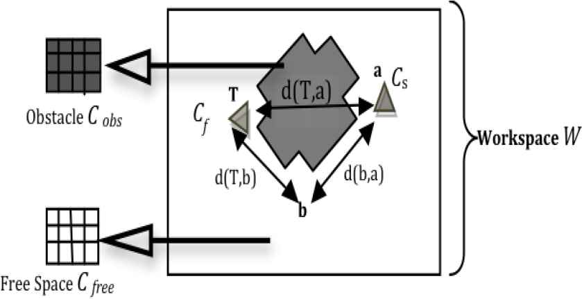
Example of the path planning domain highlighting the workspace, obstacles, free space, agent, and target.
2.2. Theoretical Background
The proposed scheme maps the free space as a distance map defined over the obstacle-free region. This distance map is analogous to a wavefront navigational function that calculates the free space map as aggregate Euclidean distances between obstacle-free states. The inspiration taken here for the navigational function is a Lyapunov-like function [34] that guarantees a valid path from any approachable state in the system to the target state. This scheme assures that the agent will not get stuck at any intermediate location before reaching the target, and the workspace map will not suffer from local minima.
Let
Let
2.3. Mapping of Free Space to Free Space Manifold
The previous section established the layout of the optimal workspace map for the path planning by defining the free space manifold. Here lies the main challenge of path planning, i.e., to map the workspace
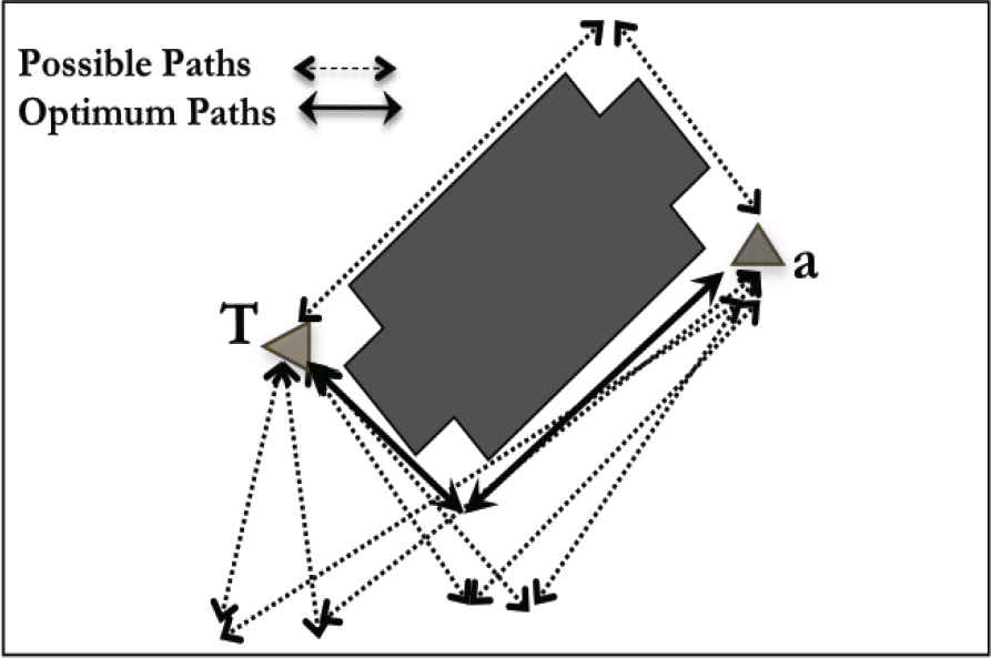
Free space mapping considering only one intermediate point. Candidate paths, out of many only few are shown as dotted lines and optimum path by solid lines.
Let
Define
The optimum choice for the states to be searched would be the ones in the immediate neighborhood, i.e.,
2.4. Workspace Model for EfficientPath Planing
The proposed system has similar setup to the Glasius model [27] which states that the value of neuron
In our work, for the workspace composed of
The
In order to address the “too close” problem an
2.5. Efficient Algorithm for OptimumPath Generation
Algorithm 1 provides the details of M2W working, here
Algorithm 1: Algorithm for M2W Path Planner
1: Initialize n states of the workspace grid with
2: Set the target state to one
3: Initialize iteration counter
4: Set maximum radius of wave
5: while There are any unmapped states or number of iterations are less than the number of states (Any(
6: Increment iteration counter
7: for Outward Wave: States form target state to the maximum radius
8: Select neighboring States
9: for all Neighboring states
10: Evaluate
11: end for
12: end for
13: for Inward Wave: States starting from maximum radius to target state k = s to 1 do
14: Select neighboring States
15: for all σj in η do
16: Evaluate
17: end for
18: end for
19: end while
Each state's value depends upon the neighboring state; the order in which the states are processed is of great importance. At the beginning of the path planning process, all states are set to arbitrarily high values to facilitate the minimum operation, and only the target state is set as one. The states in the immediate neighborhood, i.e., at the unit distance from the target, are processed first and then the ones at two units away etc. until the entire workspace is processed. The states are processed in the form of a circular wave going outward from the target state. Here the proposed algorithm is different from the navigational function [21,22] as it does not maintain any queues, so our method is more efficient in the absence of obstacles. And in lack of queues of free space, the states hidden behind concave obstacles do not get aligned to the free space by unidirectional updates. Thus the reverse wave originating from the boundary moving inward and terminating at the target state is implemented. The reverse wave not only maps the states covered by concave U-shaped obstacles, but it also helps in mapping the repulsive effect of the obstacles by using matrix
It can be seen in Eq. (9) that as
In the case of more complex obstacles, the repulsive effect is more substantial near convex structures. Figure 3a shows the
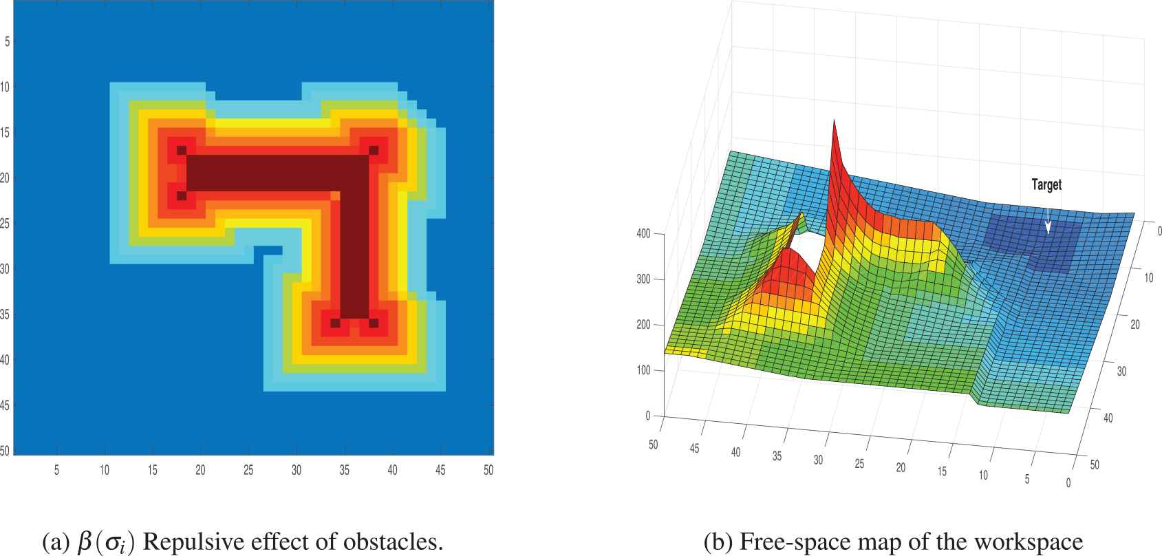
Free space mapping of mission space with an L-shaped obstacle. The mapping with safety considerations prohibits the robot from getting too close to an obstacle.
There is a possibility for the set of free states to be surrounded by the obstacle in such a way that there is no free path leading toward the target state. The current work identifies such a case by maintaining a counter of the number of iterations and forcing the algorithm to terminate if the number of iterations exceeds the number of free states. This brute force selection of the terminating criterion is adopted only to elaborate on the proposed work's worst-case scenario. In the case of extremely complex workspaces where for each update wave, backward or forward, only one state gets classified. The maximum number of iterations is not more than the number of free states in the workspace. Here counter helps in the identification of the lack of solution.
3. SIMULATIONS
In this section, we present simulated studies carried out to demonstrate the effectiveness of the proposed approach. Simulation and The four features of path planning are demonstrated in the following simulations.
U-shaped Obstacles: This case outlines the better performance of M2W in the presence of U-shaped obstacles. It is shown that a. M2W generates workspace without local minima, b. the generated paths are safe and c. the shortest.
Spiral Maze: The spiral maze path problem is simulated to elaborate the a. the strength of discretized workspace mapping and b. relation of the execution time of algorithm with the number of free states. It is shown that in the case of complex and dense workspace, the execution time of the algorithm is reduced with a reduced number of free cells.
Moving targets: The simulations show how M2W performs in a dynamic environment. Each time M2W generates optimum paths to moving the target's location.
Three Dimension: The simulation shows how M2W can easily be adopted from 2-dimensional space to three-dimensional space.
Configuration Space Planning: This simulation demonstrates the adaptability of M2W with additional constraints of object orientation.
In the following examples, the workspace is represented as a two and three-dimensional lattice. We focus on mobile robot path planning and obstacle avoidance in both static and dynamic environments. As each state searches for the free space only in the immediate neighborhood,
3.1. Case 1: U-Shaped Obstacles
The first simulation illustrates the proposed algorithm in the presence of concave obstacles. This is the typical problem where APF fails due to presence of local minima. The workspace has 2500 states arranged in a two-dimensional grid of 50 rows and 50 columns. With a single U-shaped obstacle, Figure 4, simulated results are shown to establish the performance of the path planning algorithm with respect to the complexity of concave obstacles. Figure 4 shows the comparison of APF and M2W based mapping in workspace. Here the workspace is mapped using well known harmonic APF [35].
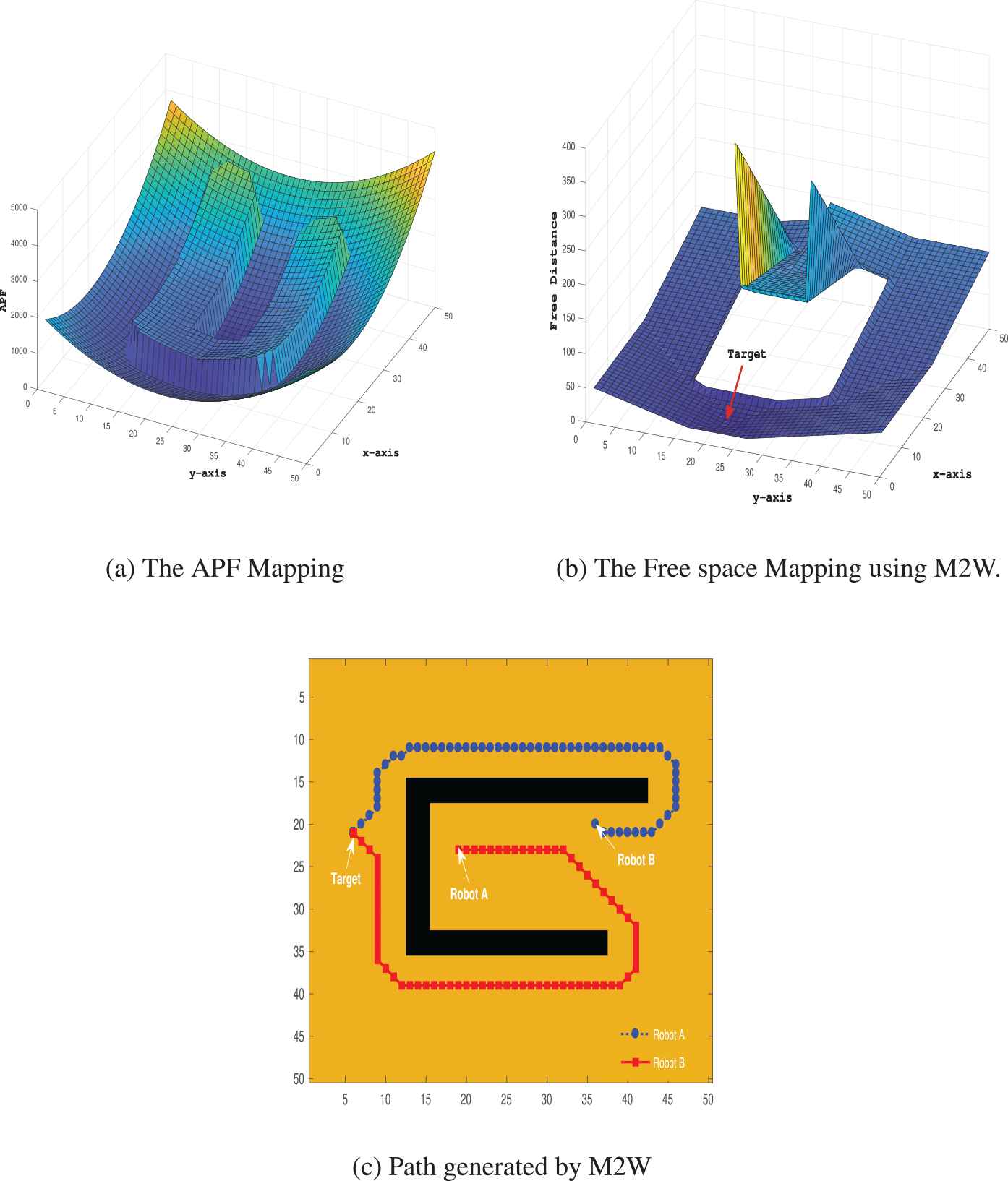
The free space mapping using Modified 2-Way Wavefront (M2W) and Artificial Potential Fields (APF). The map by M2W does not suffer from local minima where as the path generated by APF never reaches to target.
From Figure 4a, it can be seen that in the APF map, the force of attraction is stronger in the area enclosed by the obstacle than the force felt at the free path leading out from the U-shaped obstacle. This situation makes it impossible for a robot to be positioned inside the obstacle to reach the target location outside the obstacle. On the other hand, in M2W, the states are mapped as the free distance from the target location. The states enclosed by the obstacle are mapped as farther from states leading out of the obstacle. This helps M2W find a path out of the obstacle, whereas the path generated by the APF never reaches the target.
The algorithm requires one iteration, updating the workspace in both directions: firstly from target to the boundary states and then from the boundary states toward the target. Two examples are shown with different initial positions. The path generated for both robots are smooth and do not suffer from local minima. The robots reach the destination state without moving toward the obstacle, i.e., from the first step to the very last step, the path is the optimum solution under the given circumstances. Furthermore, to elaborate that the optimum paths do not pass through the states too-near the obstacles, the repulsion normalizing factor
An extreme test of the M2W is shown in Figure 4c: where the first and second optimum (shortest and safe) paths for robot A have a minimal difference in terms of distance, but very significant difference in terms of the route taken. A safe path for robot A with a starting location near to the convex region is 75 steps through the smaller arm (Figure 4c: robot A's best path) and 77 steps (Figure 4c: robot A's next best path) from the long arm. Even though it may seem that robot A has to cover longer distances, whereas, on the contrary, the robot is choosing the smaller of the two safe paths. The escape route's selection through the smaller arm instead of, the longer one is evidence of the cumulative distance-based mapping, which always results in valid optimum paths.
3.2. Spiral Maze Problem
We now demonstrate the M2W behavior on spiral maze environments (Figure 5) again with the workspace of 50
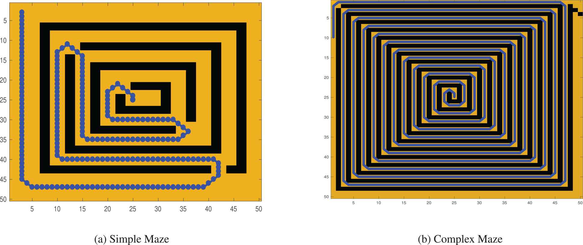
Spiral maze problem simulation.
In the second denser scenario, Figure 5b, it took 21 iterations to map the maze problem with the target location in the center of the maze. Note that out of 2500 states, 1125 states are obstacle states. Even though it took 21 iterations to generate the free space map, the maximum clearance method would have taken as many iterations as that of obstacle states.
3.3. Moving Target and Obstacles
In a situation where the target is dynamic, and the robot has the task to chase and capture the target, the sensory information in terms of the input matrix,
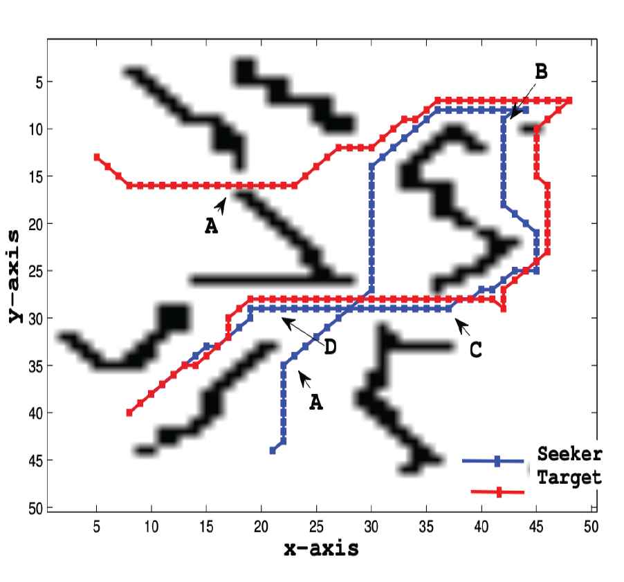
Moving Target: The path generated by using Modified 2-Way Wavefront (M2W) in pursuit of the target is stable and secure.
At point B the robot catches up to the target, but to demonstrate, the behavior of the M2W simulation does not terminate at this point. At point B, the robot's path is shorter than that of the target, thus showing that even in case of the target's zigzag movement, the seeker will have a stable straight path resulting in the seeker catching up with the target. Point C shows the seeker's path at a safe distance from the obstacle in comparison to the target that is moving very close to the obstacle. This indicates that the seeker's well-being has a priority over the capture of the target, and the seeker does not run into a potentially harmful situation while following the target.
Figure 7 shows the same workspace with a dynamic environment, having moving obstacles and moving targets. In Figure 7a, when the seeker robot approaches the point marked as A, an obstacle (shown as a black box) appears in its path, the seeker then moves toward the bottom opening near the point B. Figure 7b shows that as the seeker approaches to point B, the opening is restricted by the appearance of another obstacle. Having the path from A to B closed the seeker backtracks and moves toward the only viable opening. When it approaches point C, Figure 7c, another obstacle is introduced while the obstacle at A is removed. This dynamic behavior of the seeker shows that the proposed method is feasible for static and dynamic environments.
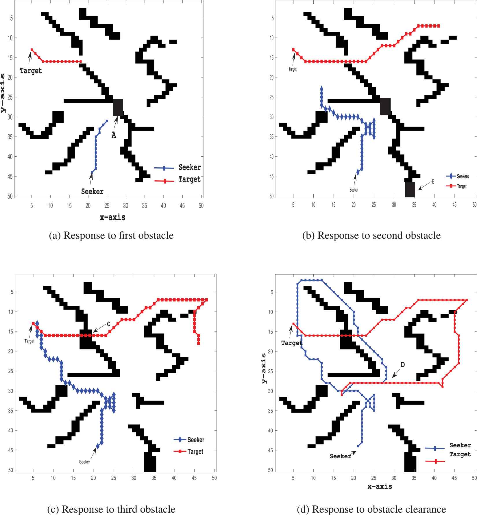
Moving target and obstacles: with obstacles appearing during the mission restricting the robots' path.
3.4. Path Planning in Three Dimensions
M2W is easily extended from two-dimensional mapping to three-dimensional mapping. The new dimension's addition may result in an increased number of neighboring states and the total number of states in the workspace. However, the algorithm performs in the same manner, even in three dimensions, and generates safe paths from source to target location. Figure 8 shows the three-dimensional workspace of size (50

Three-dimensional mapping using Modified 2-Way Wavefront (M2W) with workspace divided into four sections. The starting location's path to the target location has to go through the small windows in separating walls.
3.5. Configuration Space Planning
The path planning for a rigid body robot whose dimensions and orientation are not compatible with that of the discretized space cells is a complex problem for planner algorithms. There are many considerations to be kept in mind, such as the constraints on the motion, the selection of the orientation that best fits in a narrow path, etc. These problems are commonly known as the piano movers problem. One such problem's simulation for an L-shaped object is presented in Figure 9. Here the workspace has 400 states with 20 rows and 20 columns with the obstacles shown as solid black spaces. The
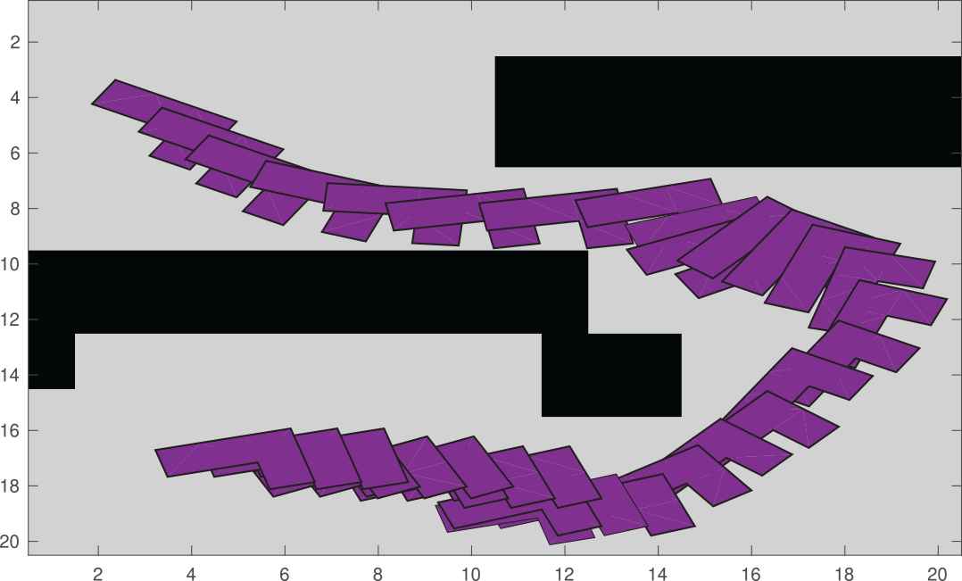
Planning for L-shaped object.
A simple modification is performed to the M2W by introducing a matrix that keeps a record of all admissible angles at a specific state. Simultaneously, while the matrix is estimated, care is taken that if all orientations of the object, i.e., all
It is evident from Figure 9 that even with these simple modifications, the M2W produces a valid smooth path for the rigid body with an initial location at the top left of the figure to the target location at the bottom.
4. CONCLUSIONS
A new and efficient method, M2W, for robotic path planning in the discretized workspace is presented. The proposed work is inspired by the navigational method, APF, and Glasius model-based path planning. It combines the salient features of all three schemes but does not suffer from any of the shortcomings.
M2W has linear complexity in terms of the number of states in the workspace. Furthermore, the linearity depends on the shape and orientation of the obstacles regarding the target location. In the case of simple obstacles, it outperforms SOM planners as it does not require any time for neurons' activity to settle. It is more efficient than crude navigational planners in the absence of the obstacles as it does not maintain any queues. M2W does not suffer from local minima. The workspace in M2W is mapped in terms of the strictly positive and increasing function of the free space metric with respect to target location acting as a stationary point/global minima.
The paths generated by M2W are safe and do not lead dangerously near to the obstacles. M2W can be used in many scenarios (2D, 3D, and configuration planning) with suitable modification. It's suitable for static as well as the dynamic environment. For future work the M2W is extended for multiple co-operative agents by incorporating collective performance indicators, e.g., communication, task decomposition, uncertainty, and multiple targets.
CONFLICTS OF INTEREST
The authors declare that they have no conflicts of interest to report regarding the present study.
AUTHORS’ CONTRIBUTIONS
All authors contributed equally.
Funding Statement
The author(s) received no specific funding for this study.
REFERENCES
Cite this article
TY  - JOUR
AU  - Ayesha Maqbool
AU  - Alina Mirza
AU  - Farkhanda Afzal
PY  - 2021
DA  - 2021/03/15
TI  - Modified 2-Way Wavefront (M2W) Algorithm for Efficient Path Planning
JO  - International Journal of Computational Intelligence Systems
SP  - 1066
EP  - 1077
VL  - 14
IS  - 1
SN  - 1875-6883
UR  - https://doi.org/10.2991/ijcis.d.210305.002
DO  - 10.2991/ijcis.d.210305.002
ID  - Maqbool2021
ER  -