
Rumor Detection by Propagation Embedding Based on Graph Convolutional Network
 , Jason J. Jung*,
 - DOI
- 10.2991/ijcis.d.210304.002How to use a DOI?
- Keywords
- Rumor detection; Propagation embedding; Graph convolutional network; Feature aggregation
- Abstract
Detecting rumors is an important task in preventing the dissemination of false knowledge within social networks. When a post is propagated in a social network, it typically contains four types of information: i) social interactions, ii) time of publishing, iii) content, and iv) propagation structure. Nonetheless, these information have not been exploited and combined efficiently to distinguish rumors in previous studies. In this research, we propose to detect a rumor post by identifying characteristics based on its propagation patterns and other kinds of information. For the propagation pattern, we suggest using a graph structure to model how a post propagates in social networks, allowing useful knowledge to be derived about a post's pattern of propagation. We then propose a propagation graph embedding method based on a graph convolutional network to learn an embedding vector, representing the propagation pattern and other features of posts in a propagation process. Finally, we classify the learned embedding vectors to different types of rumors by applying a fully connected neural network. Experimental results illustrate that our approach reduces the error of detection by approximately 10% compared with state-of-the-art models. This enhancement proves that the proposed model is efficient on extracting and integrating useful features for discriminating the propagation patterns.
- Copyright
- © 2021 The Authors. Published by Atlantis Press B.V.
- Open Access
- This is an open access article distributed under the CC BY-NC 4.0 license (http://creativecommons.org/licenses/by-nc/4.0/).
1. INTRODUCTION
Social networks (e.g., Facebook and Twitter) are currently the most common media platforms for monitoring and broadcasting news across the world. While news from other media platforms (e.g., newspapers and television channels) are published by recognized organizations and are thoroughly verified after many censor steps, most of the information in social networks is published by individuals. The individuals may publish news based on their personal perspectives. Additionally, many people intentionally publish fake information to attract attention or achieve their purpose. Besides, they do not have to take responsibility for their published information, and most social networks do not take any steps to verify information before publication. Therefore, many posts in these networks are rumors, fake stories, or misinformation. This leads to the spread of improper information, which can cause detrimental effects on individuals and organizations.
By common definition, a rumor is a statement whose truth value is unverified [1]. Rumor detection is an important task to ensure the truthfulness of the information on social media platforms. Therefore, the task of detecting rumors needs an examination of a huge amount of information for checking the credibility of the suspected statement. There are various online services (e.g., Snopes,1 and PolitiFact2) that support debunking rumors. However, these services require manual fact-checking by analyst specialists. This process is highly labor-intensive and time-consuming. Therefore, an automated and real-time rumor detector must be developed.
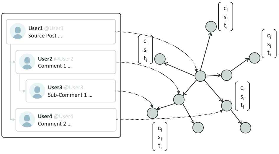
For automatically detecting rumors, most previous research have focused on extracting set of handcrafted features from the user profile, post content, and propagation patterns [2,3]. More recently, several studies have applied deep neural networks for auto-learning features [4,5]. Mostly such studies neglect or oversimplify the propagation structure, although it has been shown to be effective in identifying rumors. The propagation structure of a post is known as how a source post reaches other people in social networks. When a post is published on social networks, it is delivered to the author's subscribers, who can then respond by response posts (e.g., comments, retweets, or shares) to express their opinions about the source post. Recent studies show differences between behavior of people and semantic relationship between the posts in a propagation process. For example, Ma et al. [6] assume that if a post is a rumor, it could receive many negative responses (e.g., “disagreement” or “blame”), whereas a nonrumor post is likely to have many positive responses (e.g., “agreement” or “support”). Figure 1 gives an example of how people express their stance toward a tweet on Twitter. This tweet is a rumor because there is no official organization that confirms the truthfulness of its content at the time of publishing. Most comments on this tweet express suspicion or disagreement. Specifically, the comments of “User2” and “User4” express suspicion. The comment of “User3” expresses disagreement. This observation is a motivation for us to develop a rumor detection method by learning the difference in how different posts respond to the source post in the propagation process.

Example of a rumor tweet propagating on Twitter. Most comments on this rumor express suspicion or disagreement.
In this study, we propose a novel method to incorporate the propagation structure and other derived features into a graph [7], where each node is either the source post or responses (e.g., comments), and each edge represents a relationship between posts. Features extracted from a post are attributes of its corresponding node. The features can be extracted from the content, temporal, and social information of a post. By using a graph to represent the propagation structure and valuable features of a post, the rumor classification problem is transformed into the graph classification problem. There are many graph classification algorithms which were proposed based on graph kernels [8,9], or spectral and statistical fingerprints [10]. However, these methods are not suitable or not applicable to our constructed graph. Therefore, we propose using a graph embedding approach which embeds the constructed graph into a continuous vector space. Next, we classify these graph embedding vectors by using a supervised classification model.
For graph embedding, there exist various methods for learning node embedding (e.g., DeepWalk [11], node2vec [12], SDNE [13]), subgraph embedding (e.g., subgraph2vec [14]), and full graph embedding (e.g., graph2vec [15]). However, the weakness of these algorithms is that they only focus on embedding structural information but forget to learn the features of nodes and edges. Instead, we propose a graph embedding model based on a Graph Convolutional Network (GCN) [16] and Long Short-Term Memory (LSTM) network [17], which allows embedding full graph features without loss of information. The GCNs allow to leverage both the node features and the graph structure to generate node embeddings for previously unseen data. By using the GCNs, the learned node embedding is a combination of the structural information and the node features. The GCN that we use is GraphSAGE [18]. GraphSAGE is an inductive variant of GCNs, which uses trainable aggregator functions instead of simple convolutional function. We then apply an LSTM model for learning the graph embedding vector from the sequence of node embeddings. Next, we classify these graph embedding vectors to rumor labels by a fully connected neural network.
Finally, we evaluate the proposed model on public Twitter datasets. The experimental results indicate that our model outperforms strong baseline models. The main contributions of our study are summarized as follows:
We propose a method to model the propagation process of a post as a graph. This allows learning the structural information of the propagation process by using a GCN.
A graph embedding method is applied to integrate both the graph structure information and the node features to extract valuable signals to detect rumors. Additionally, this technique is strong in generalizing unseen data because the propagation structure varies for different posts.
A semi-supervised training method is proposed to exploit a high volume of unlabeled data in social networks and enhance the model's performance in the case of a lack of labeled training datasets.
Our model demonstrates state-of-the-art performance on real-world datasets for the rumor detection task.
The rest of the paper is organized as follows. Section 2 summarizes previous research on rumor detection and graph embedding techniques. The rumor detection problem is described in Section 3. Section 4 explains the proposed model. Section 5 presents the datasets, experiments, and results. In Section 6, the conclusions and the scope for future research are given.
2. RELATED WORK
In this section, we summarize relevant approaches to rumor detection. In addition, we discuss some studies on graph embedding and explain the reason why GraphSAGE is more suitable than other embedding methods for our approach.
2.1. Rumor Detection
The problem of rumor detection has been an important subject of research when social networks become popular. In an early study, Zhao et al. [19] defined a set of regular expressions to detect signal posts that express inquiry about the truth value of post. The drawback of this approach is that it heavily depends on predefined regular expressions, which cannot encompass the diversity of writing styles used in posts. Similarly, many early studies focused on training a supervised classifier based on manually extracting features from post's information [2,3,20–23]. The disadvantage of these approaches is their strong reliance on the method of feature engineering, which is likely to be biased and labor-intensive.
Another research approaches leverage the propagation patterns of the tracked posts. Kwon and Cha [24] proposed an approach based on monitoring the difference between the propagation patterns. Recently, by integrating the post features based on calculating the weight of each post using the PageRank method, Vu and Jung [25] embedded the propagation process and then categorized the embedding vectors according to rumor labels. Furthermore, some kernel-based approaches were proposed to differentiate the propagation structure of rumor and nonrumor posts. Wu et al. [26] introduced a graph-based kernel function to capture propagation patterns and semantic features of posts, and Ma et al. [27] proposed a tree-kernel function that learns the similarity between propagation trees by evaluating the similarity of sub-trees. However, these methods have highly computational complexity because it needs to calculate the similarity between every pair of graphs or trees.
Recently, several studies of rumor detection centered on developing a neural network model. Alkhodair et al. [4] trained a LSTM model, which only learns the source post's content to classify rumors. Ma et al. [28] introduced a recurrent neural network (RNN) to capture variations of contextual information of posts when propagating. Also, Ma et al. [6] model the propagation process as a tree and then applied a Tree-structured Recursive Neural Network to aggregate high-level information from the source and response posts. However, the tree structure only allows modeling one-to-one relationships between posts. In several social networks, a post can respond to more than one post at a time. Using the tree form therefore oversimplifies the complexity of the propagation. In addition, this tree-structured neural network enables only one path for synthesizing features: bottom-up or top-down.
Compared with previous studies, our approach is more natural and general. It relies on a graph embedding method, which allows generating representations from both neighbor structure and features by using aggregator functions in the GraphSAGE.
2.2. Graph Embedding
Graph embedding methods learn to represent a graph or its components (e.g., nodes, edges, and subgraphs) as vectors in a low-dimensional continuous space [29]. For node embedding, Perozzi et al. [11] proposed the DeepWalk model, which uses random walks to sample neighbor nodes, and trained a skip-gram model [30] to learn embeddings. Similarly, Grover and Leskovec [12] trained the node2vec model with a modification in the random walk algorithm to better preserve the network neighborhoods of nodes. Tang et al. [31] and Wang et al. [13] proposed different methods to learn node embeddings with an objective is to preserve first-order and second-order proximity, which represented local and global network structure, respectively.
For subgraph embedding, Narayanan et al. [14] proposed a model to embed subgraphs based on the maximum likelihood of co-occurrence of rooted subgraphs sharing the same context. For graph embedding, Narayanan et al. [15] introduced the graph2vec model, which samples a set of subgraphs in a graph, and then trained a skip-gram model to maximize the probability of predicting subgraphs that exist in a graph. However, these methods learn a specific vector for each node or graph; therefore, they cannot predict embeddings for a new node or graph. In contrast, the GraphSAGE learn an aggregator function that can integrate node features with the graph structure and predict embeddings for unseen nodes. This makes it perfectly suitable for the propagation graph of a post when each node has unique features, and each graph has a unique structure.
3. PROBLEM DESCRIPTION
In this section, we describe rumors and their types. We also define the propagation graph and formulate the rumor detection problem.
3.1. Definition of Rumors
A rumor is defined as a story or a statement circulating without verification or certainty of facts [1]. This means that when these stories are published, there are no reliable source confirm their trustfulness. Although the reliability of a rumor is uncertain, a rumor is not necessarily false. A post that expresses true information may still be a rumor if no trusted authority has confirmed it yet. Hence, rumors may eventually contain true or false information. Generally, rumor and nonrumor posts can be defined as follows:
Nonrumor: for a nonrumor post, the veracity of information contained in the post is verifiable at the time when it is published.
Rumor: a rumor is a post containing information that cannot be verified at the beginning of circulation.
Additionally, a rumor can be distinguished by three types: true rumor, false rumor, and unverified rumor, depending on the time this information has been confirmed after circulation [27]. These three sub-types of rumor can be defined as follows:
True rumor: a rumor that cannot verify during the first stage of spreading but was officially confirmed as true after a time period.
False rumor: information that was unverified at the beginning of circulation, then it is disproved later.
Unverified rumor: unverifiable information during the entire circulation time.
3.2. Rumor Detection Problem
In this study, we focus on classify a post into four types of rumor: nonrumor, true rumor, false rumor, or unverified rumor. This section describes a formal problem formulation. An important feature type that generalizes the whole diffusion process of a post is the propagation structure. When a post is propagated on social networks, its readers can react with response posts (e.g., comments, or shares) to express their opinions. Therefore, the propagation structure includes “response relationships” among the source post and the responses. For example, it may include the stance of a response post toward its parent post. Specifically, if a post is a false rumor, some direct response posts are likely to express the opposite stance; otherwise, if a post is nonrumor, the direct responses will likely to express a supportive opinion. Therefore, we model the propagation structure of the source post and its related responses as a propagation graph for learning the relationship between posts.
Definition 1. [Propagation Graph]
Propagation graph
For instance, Figure 2 demonstrates how we model the tweet propagation process as a propagation graph. At the beginning, “User1” posts a new tweet
Graph model of the propagation structure of a post. The posts correspond to nodes, and relations between posts are modeled as graph edges.
| Categories | Features | Descriptions |
|---|---|---|
| Content features | Embedding vector | Embedding vector of the post content |
| Capital letters ratio | Ratio of capital letters over the total number of letters in the post content | |
| Exclamation mark | Whether the post content includes an exclamation mark | |
| Question mark | Whether the post content includes a question mark | |
| Period mark | Whether the post content includes a period mark | |
| Word count | Number of words in the post content | |
| Social features | Account age | Number of years since the user account has been created |
| Post count | Number of posts published by the user account | |
| Friend count | Number of friends of the user account | |
| Follower count | Number of followers of the user account | |
| Is verified | Whether the user account is verified as an authentic account | |
| Temporal features | Time delay | Time delay between publishing time of the source post and its responses |
Examples of features that can be extracted from a post.
After embedding the propagation structure and valuable features of the posts in a graph, our rumor detection task becomes classifying the created graphs to the rumor classes.
Definition 2. [Rumor Detection]
Rumor detection is the task of learning a classifier
To classify propagation graphs, we propose a graph embedding method based on GraphSAGE and an LSTM model to learn an embedding vector for each graph. Then, these vectors are classified by using a fully connected neural network.
4. RUMOR DETECTION VIA PROPAGATION GRAPH EMBEDDING
In this section, we explain the method of rumor detection based on the classification of the propagation graphs. Figure 3 describes the overall algorithm of learning the embeddings and classifying the propagation graphs. First, we learn the node embedding vectors by aggregating the features of neighboring nodes. Then, we apply an LSTM model to learn the graph embedding vectors. Finally, we classify the graph embedding vectors by a fully connected neural network. Our model's main goal is to effectively combine the structure of propagation with the posts' internal features to output a graph embedding vector. As a result, the learned graph embedding vector is the combination of features useful for differentiating rumor posts.
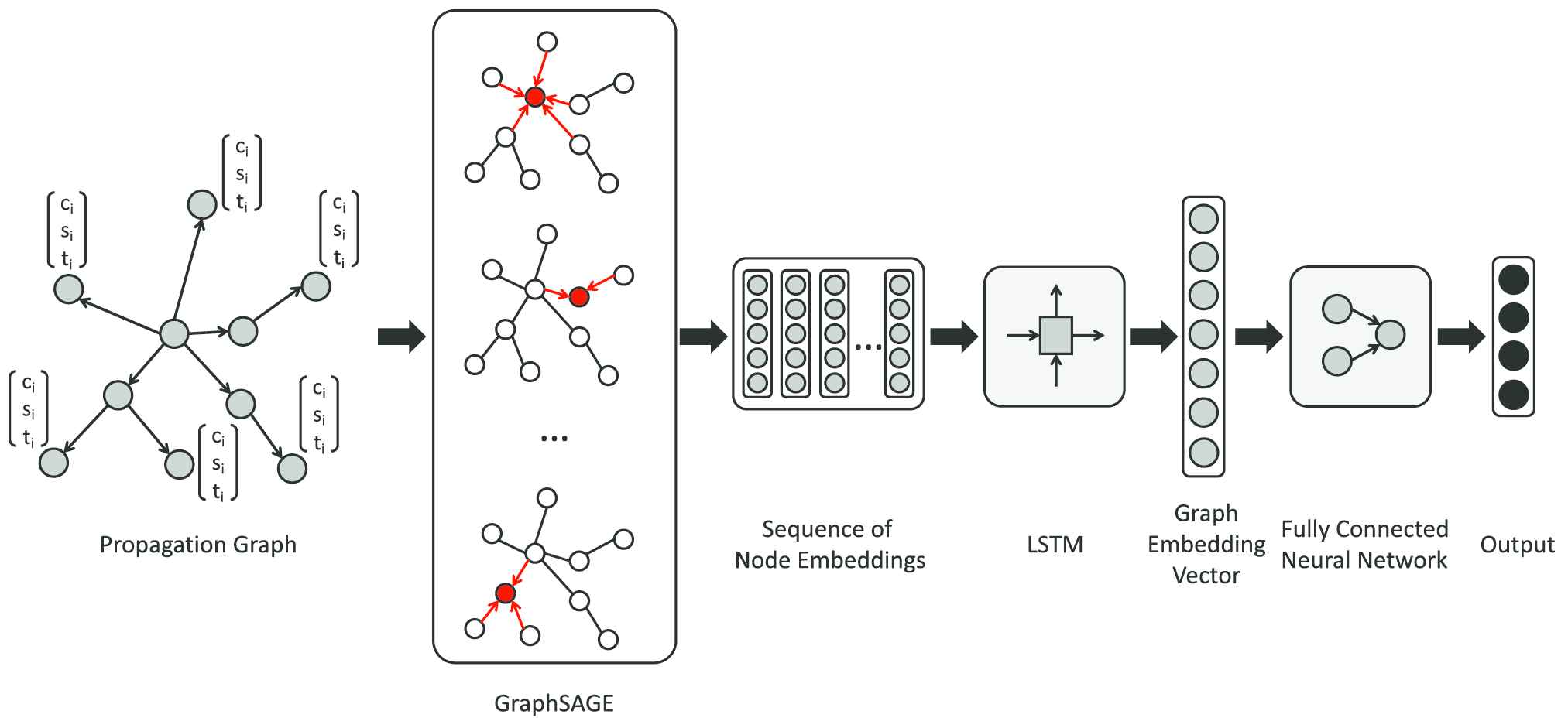
Model structure of classifying propagation graph. From the propagation graph, the node's embedding are learned by aggregating features of neighboring nodes. Then, the sequence of node embeddings is transformed by an Long Short Term Memory (LSTM) model to output graph embedding vector. Finally, this graph embedding vector is classified by a fully connected neural network.
4.1. Embedding Propagation Graph
Given a propagation graph, our task is to learn an embedding vector of this graph. The first step is to learn node embedding vectors of the propagation graph by aggregating the neighbor's features. The neighbors of a node (which represents a post) include the nodes that represent not only responses but also previous posts to which this post responds to. The purpose of this step is to learn relationships between the posts in a propagation process. For this purpose, we apply a GCN called GraphSAGE, which aggregates the internal features of nodes and the local neighbor's features into a node embedding vector. Although GraphSAGE aggregates node embeddings based on features, theoretical analysis proved that it can learn structural information regarding a node's role in a graph [18]. Next, we apply an LSTM model to learn a graph embedding vector from the sequence of node embeddings. The LSTM model includes a sequence of connected units, and each unit is responsible for processing an input vector; therefore, it can capture the whole context across the input sequence.
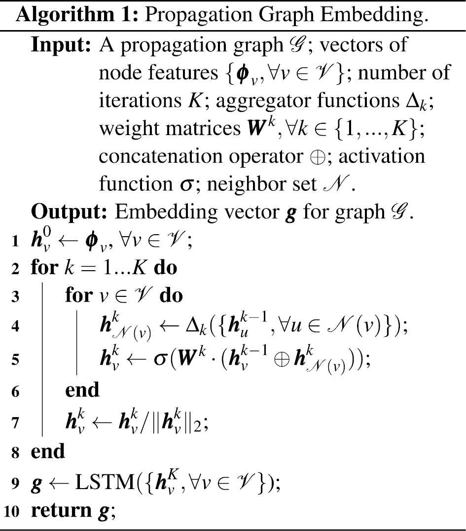
Algorithm 1 describes the procedures to generate the embeddings of propagation graphs. The input is a graph
4.2. Aggregator Functions
The aggregator functions are designed to efficiently aggregate features from a node's neighbors. In practice, the following functions are used:
Mean aggregator: Mean aggregator is the element-wise mean of the neighbors' vectors [18].
Convolutional aggregator: This aggregator takes the element-wise mean of a node's vector and its neighbors' vectors [18].
Compared with the pseudo-code of Algorithm 1, the convolutional aggregator takes both the node vector and its neighbors as inputs; further, it does not perform the concatenation step in line 5 of the algorithm.
LSTM aggregator: This aggregator applies an LSTM neural network to aggregate information across a node's neighbors [18].
Pooling aggregator: This aggregator feds each neighbor's vector through a fully connected neural network; then, an element-wise max-pooling operation is applied [18].
In the aggregator functions above, all neighbor nodes are handled equally because the features of each neighbor of a node are combined with the equal weight. However, in the propagation process, each post expresses different information; thus, its contribution to the aggregating feature process can be different. Therefore, we propose a linear aggregator function that combines neighbor feature vectors linearly based on the role of each node in the propagation graph.
Linear aggregator: The linear aggregator function is modeled as follows:
To calculate the PageRank of nodes in the propagation graph, we reverse the direction of edges from a response post to its direct target post. This edge direction follows the rule of creating a graph of webpages in the PageRank algorithm: the direction of edges in the graph is from a page to its mentioned page. Similarly, in the propagation process, the response post also mentions the target post. In such a graph, the source node is likely to have the highest Page Rank. Moreover, if a post has a high number of responses, its Page Rank is expected to be higher than for the posts with fewer responses. As a result, the source post and the response posts which are highly responded will contribute more to the aggregation process. In general, this linear aggregator with PageRank allows exploiting the nodes' importance in the graph to improve the process of feature aggregation.
4.3. Classification of the Propagation Graph
Out next task is to classify propagation graph embeddings according to the rumor labels. We classify these embedding vectors by applying a two-layer fully connected neural network. The number of neurons in the input layer is the size of the graph embedding vector. The number of neurons in the output layer equals the number of labels. The input of the network is the embedding vector, and the activation function in the output layer is the softmax function. For training model, the proposed model can be trained in a semi-supervised or supervised manner.
Semi-Supervised: In the semi-supervised setting, we learn the node embeddings in an unsupervised manner by using a set of unlabeled graph data from social networks. The loss function for unsupervised training of node embeddings is defined in GraphSAGE as follows [18]:
Supervised: In the supervised setting, the model is trained in an end-to-end manner. The parameters in the node embedding, graph embedding, and graph classification parts of the model are simultaneously updated by backpropagation algorithm in each optimization step. This model is trained to minimize the cross-entropy loss function in equation 12. This training method optimizes the embedding model and classification model specifically for the rumor detection task.
5. EXPERIMENTS AND RESULTS
In this section, we describe the training datasets, our experimental settings and results.
5.1. Datasets
In our experiments, we evaluate the proposed model on three datasets: Twitter15, Twitter16 [27], and PHEME [33]. These datasets is collected tweets, response tweets (replies and retweets), and propagation structure on Twitter. The source tweets in Twitter15 and Twitter16 datasets are annotated with one of the four class labels: nonrumor, true rumor, false rumor, and unverified rumor. Each source tweet in PHEME dataset is assigned to one of the two classes: nonrumor and rumor. Although the PHEME dataset contains only two classes, it can still be used to verify the proposed model and compare its performance with other models.
Besides, while the PHEME dataset provides JSON files with detailed information on each tweet, Twitter15 and Twitter16 only provide the tweet ID without content and other information; therefore, we use the Twitter API3 and Tweepy library4 to query content and social information from the tweet ID. Besides, Twitter15 and Twitter16 have a similar structure; therefore, we merge them into one dataset called Twitter15 + Twitter16 and train our model on this dataset. Table 2 shows statistics of the training datasets. The number of source and response tweets in Twitter15 and Twitter16 are the tweets that we could query by ID. Moreover, some tweets appear in both Twitter15 and Twitter16; hence, the number of tweets in Twitter15 + Twitter16 is smaller than the total number of tweets in Twitter15 and Twitter16. Furthermore, we removed the retweets from the propagation graph because the content in retweets is mostly empty, and they do not provide any valuable information.
| Statistic | Twitter15 | Twitter16 | Twitter15 + Twitter16 | PHEME |
|---|---|---|---|---|
| Number of source tweets | 1,490 | 818 | 2,139 | 6,425 |
| Number of response tweets | 42,500 | 19,290 | 57,649 | 98,157 |
| Number of nonrumor tweets | 374 | 205 | 579 | 4,023 |
| Number of false-rumor tweets | 370 | 205 | 575 | |
| Number of true-rumor tweets | 372 | 207 | 579 | 2,402a |
| Number of unverified-rumor tweets | 374 | 201 | 406 | |
| Average number of tweets / graph | 29.5 | 24.6 | 28.0 | 16.3 |
| Min number of tweets / graph | 1 | 1 | 1 | 1 |
| Max number of tweets / graph | 324 | 285 | 324 | 346 |
This value denotes the total number of rumors, (including true, false, and unverified rumors).
Statistics of the training datasets.
5.2. Feature Extraction and Text Preprocessing
In our experiments, we use extracted features that are described in Table 1. The extracted features are concatenated to obtain a feature vector of a node. However, values of the following features: account age, post count, follower count, friend count, and word count vary over different ranges; therefore, we apply a Min-Max transformation to normalize their values to range
To learn the embedding vector of a tweet's content, we use the Word2vec [30] model to learn the embedding vector of each word, and then calculating element-wise average of these word vectors in the content string. However, the content of a tweet is extremely noisy because it usually includes many abbreviations, typographical errors, and special characters. Furthermore, tweet content may include special components (such as hashtags, URLs, emails, emojis, dates, and time). Hence, to improve the performance of training the embedding models, the tweet need to clean beforehand.
We clean the tweet content through 6 steps: i) lower-case conversion, ii) special strings annotation (e.g., “URL,” “email,” “phone number,” “time,” “data,” and “number”), iii) spelling correction, iv) emoji mapping, v) removing stop words, and vi) stemming and lemmatization. In the special string annotation step, we attempt to map each special string to its string type (e.g., we map all URLs in a tweet to an “URL” string, and all emails to an “email” string). This helps the embedding algorithm learn a unique vector for different variations of a type of a special string. The spelling correction step is used to correct misspellings, which are very popular in social media texts. The emoji mapping step is to convert each emoji to a string with a representative emotion (e.g., “:-)” is mapped to “happy,” and “:-(” is mapped to “sad”). The stop-word removal step aims to remove stop words that do not express additional meaning in the sentence. Finally, the stemming and lemmatization step is used to convert a string from all different morphological variations to its common base form. To annotate special strings, correct misspelling errors, and convert emojis, we use Ekphrasis [34], which is a text-processing library for cleaning text from social networks (e.g., Twitter and Facebook). Additionally, we use NLTK [35], which is a popular toolkit for natural language processing tasks, to perform the stop-word removal, stemming, and lemmatization steps.
5.3. Experimental Settings
To evaluate the performance of the proposed model, we made a comparison with strong baselines and recent state-of-the-art models. The compared models are selected to have different approaches, from a simple model that extracts handcrafted features to more advanced models that apply modern deep-learning techniques.
SVMC: Castillo et al. [2] applied an SVM classifier to detect rumors based on hand-crafting features from the post content, user profile, discussion topic, and propagation patterns.
DTR: Zhao et al. [19] proposed a ranking model by searching for signal posts and then applying a Decision Tree model to rank the likelihood of being a rumor.
RFC-AVG: A baseline model we built by averaging the feature vectors of all nodes in the graph to output the propagation vector. Then, this vector is classified by using the Random Forest model.
RFC-PR: This model learns an embedding vector that represents the propagation structure based on PageRank. Subsequently, a Random Forest classifier is trained to classify these vectors [25].
RvNN: Ma et al. [6] modeled the rumor propagation as a tree and then they trained a Tree-structured Recursive Neural Network to detect them.
We train our model with five variants of aggregator functions to compare their performance in rumor detection. In addition, we train our model in both semi-supervised and supervised manner. In the semi-supervised setting, we train the node embedding model on the extracted graph data from the both training datasets: Twitter15 + Twitter16 and PHEME. We name the training variants as follows: SSGE-mean, SSGE-conv, SSGE-lstm, SSGE-pooling, and SSGE-linear for semi-supervised learning with mean, convolutional, LSTM, pooling, and linear aggregator function, respectively; and SGE-mean, SGE-conv, SGE-lstm, SGE-pooling, and SGE-linear for supervised learning with mean, convolutional, LSTM, pooling, and linear aggregator functions, respectively.
We use PyTorch [36] to implement models and the Adam with weight decay (AdamW) [37] to optimize parameters. We train our model using the batch training method with a batch size of
5.4. Results and Analysis
In this section, we describe and analyze the results of our model and other models.
5.4.1. Performance of rumor detection
Table 3 compares the performance of our model with other models on the Twitter15 + Twitter16 and PHEME datasets. In general, the proposed model performs better than other models via embedding valuable information in the propagation process.
| Model | Twitter15 + Twitter16 |
PHEME |
||||||||
|---|---|---|---|---|---|---|---|---|---|---|
| Accuracy | Macro-F1 | NR |
TR |
FR |
UR |
Accuracy | F1 | Precision | Recall | |
| F1 | F1 | F1 | F1 | |||||||
| SVMC | 0.422 | 0.374 | 0.614 | 0.390 | 0.368 | 0.123 | 0.639 | 0.243 | 0.563 | 0.155 |
| DTR | 0.412 | 0.398 | 0.588 | 0.433 | 0.367 | 0.204 | 0.553 | 0.415 | 0.407 | 0.424 |
| RFC-AVG | 0.665 | 0.639 | 0.734 | 0.726 | 0.629 | 0.465 | 0.793 | 0.698 | 0.770 | 0.637 |
| RFC-PR | 0.704 | 0.696 | 0.688 | 0.801 | 0.676 | 0.618 | 0.817 | 0.741 | 0.789 | 0.699 |
| RvNN | 0.744 | 0.734 | 0.815 | 0.791 | 0.718 | 0.612 | 0.825 | 0.765 | 0.772 | 0.760 |
| SSGE-mean | 0.752 | 0.743 | 0.800 | 0.796 | 0.730 | 0.648 | 0.838 | 0.781 | 0.792 | 0.773 |
| SSGE-conv | 0.727 | 0.721 | 0.783 | 0.774 | 0.688 | 0.638 | 0.834 | 0.779 | 0.775 | 0.784 |
| SSGE-lstm | 0.690 | 0.674 | 0.767 | 0.779 | 0.629 | 0.519 | 0.840 | 0.785 | 0.787 | 0.786 |
| SSGE-pooling | 0.738 | 0.727 | 0.803 | 0.784 | 0.702 | 0.617 | 0.826 | 0.770 | 0.763 | 0.780 |
| SSGE-linear | 0.759 | 0.751 | 0.805 | 0.805 | 0.733 | 0.662 | 0.834 | 0.776 | 0.785 | 0.770 |
| SGE-mean | 0.754 | 0.745 | 0.812 | 0.797 | 0.735 | 0.636 | 0.842 | 0.795 | 0.772 | 0.820 |
| SGE-conv | 0.751 | 0.742 | 0.791 | 0.811 | 0.704 | 0.662 | 0.840 | 0.782 | 0.796 | 0.771 |
| SGE-lstm | 0.704 | 0.696 | 0.767 | 0.756 | 0.674 | 0.588 | 0.842 | 0.794 | 0.778 | 0.811 |
| SGE-pooling | 0.729 | 0.715 | 0.813 | 0.783 | 0.704 | 0.559 | 0.824 | 0.761 | 0.772 | 0.755 |
| SGE-linear | 0.770 | 0.763 | 0.819 | 0.821 | 0.731 | 0.682 | 0.841 | 0.786 | 0.794 | 0.779 |
The bold numbers indicate the best results.
Performance comparisons between models on Twitter15 + Twitter16 and PHEME datasets.
According to the results, the performance of the two first baseline models (i.e., SVMC and DTR), which are based on handcrafted features, is significantly low in both training sets. The RFC-AVG method performs relatively well, with an accuracy of
However, the proposed model outperforms all baseline models on both datasets for most aggregator functions. For the Twitter15 + Twitter16 dataset, the proposed model, which uses the mean, convolutional, and linear aggregator, achieves a better accuracy than the best baseline model RvNN. Besides, the model using the linear aggregator, which is trained in the supervised manner, achieves the best results in terms of accuracy, macro-F1, and F1 score for three classes (nonrumor, true rumors, unverified rumors). The supervised model using the mean aggregator gives the best F1 score in predicting false rumors. For the PHEME dataset, the supervised model applying the mean and LSTM aggregators has the best accuracy of
In our model, supervised learning generally outperforms semi-supervised learning for all aggregator functions except for the pooling one. This is because the node embedding model in semi-supervised learning is optimized for a different objective function. However, the semi-supervised models can prove their advantage when the size of labeled training data is small (see Section 5.4.2). Comparing the models that apply different aggregator functions in the semi-supervised training method, the linear aggregator function outperforms other aggregator functions, whereas the LSTM aggregator function has the lowest performance in the Twitter15 + Twitter16 dataset. For the PHEME dataset, the best and the worst semi-supervised models are the models using the LSTM and pooling aggregator, respectively. In the supervised training method, the model using linear aggregator function outperforms other aggregator functions on the Twitter15 + Twitter16 dataset. Besides, the model using the LSTM aggregator performs worst in this dataset. However, the models using the mean and LSTM aggregator functions achieve the best accuracy for PHEME. In contrast, the model using pooling aggregator function has the lowest performance among aggregator functions.
5.4.2. Comparison between semi-supervised and supervised models
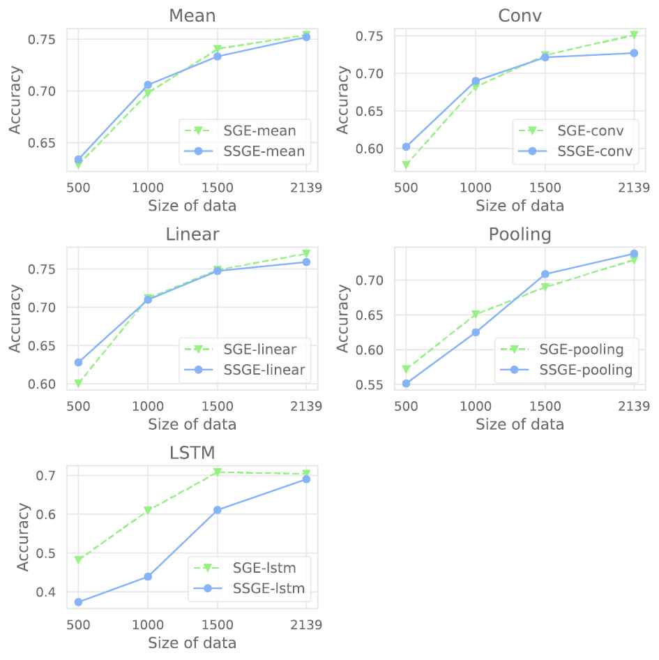
To compare semi-supervised and supervised learning methods when the size of a training dataset is small, we train the model with different sizes of training data. Figures 4 and 5 illustrate the accuracy of semi-supervised and supervised models with different sizes of data in the Twitter15 + Twitter16 and PHEME datasets. In the Twitter15 + Twitter16 dataset, we randomly pick 500, 1000, 1500, and all items for training. In the PHEME dataset, we randomly choose 1000, 3000, 5000, and all items for training.
Comparison between semi-supervised and supervised models for the Twitter15 + Twitter16 dataset.
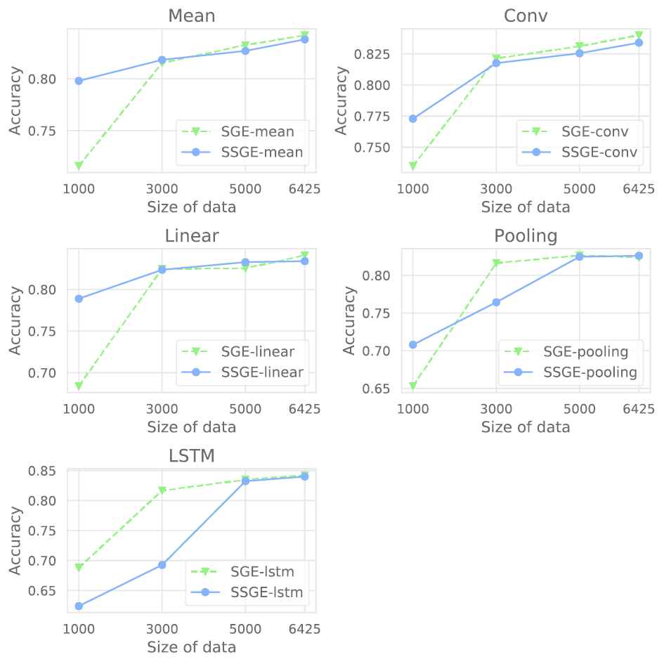
Comparison between semi-supervised and supervised models for the PHEME dataset.
For Twitter15 + Twitter16, the accuracy of semi-supervised models is better than of supervised models using the mean, convolutional, and linear aggregator functions when the size of training data is small (500 items). When the number of training samples increases, the accuracy of the supervised models increases at a faster pace. The supervised models then outperform the semi-supervised models when training on the full-size training dataset. For the PHEME dataset, when training with 1000 items, the semi-supervised models using mean, convolutional, pooling, and linear aggregator functions outperform the supervised models by a large margin. However, when training with the full-size dataset, the supervised models outperform semi-supervised ones. Hence, these experimental results prove that the semi-supervised training method can be applied when the size of the training dataset is small. Moreover, we see that the models' performance increase when the number of training items increases in all models using different aggregator functions in both datasets.
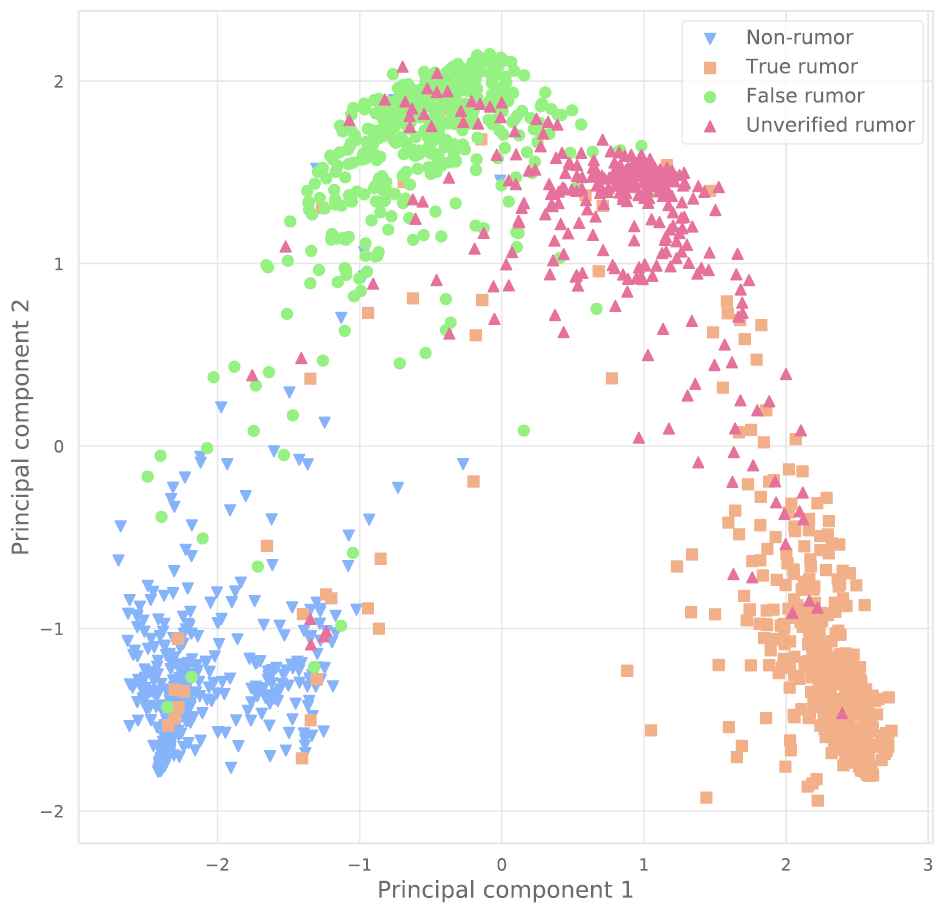
5.4.3. Visualization of graph embedding vectors
Our model learns an embedding vector for each propagation graph to combine valuable features in the propagation process of a post before classifying them. Figures 6 and 7 elucidate the distribution of the learned graph embedding vectors in a two-dimensional space in the Twitter15 + Twitter16 and PHEME, respectively. To visualize the graph vectors, we apply the Principal component analysis (PCA) [38] technique to reduce the dimensions of the graph vectors. Here, the graph embedding vectors with different labels are distributed to separate clusters in both datasets: Twitter15 + Twitter16 and PHEME. This proves that the learned graph embedding vectors include meaningful features to differentiate rumors. However, for Twitter15 + Twitter16, the cluster of graph vectors for unverified rumors slightly overlaps with the clusters of vectors for true and false rumors. This shows that the features of unverified rumors and true/false rumors are relatively similar. This also explains why the F1 score of all models when predicting unverified rumors is lower than for other types of rumors.
Visualization of distribution of graph embedding vectors for the Twitter15 + Twitter16 dataset.

Visualization of distribution of graph embedding vectors for the PHEME dataset.
5.4.4. Comparison between embedding methods
To illustrate the efficiency of the proposed propagation graph embedding method, we compare performance between our proposed method and other node embedding algorithms (i.e., DeepWalk [11], node2vec [12], LINE [31], and SDNE [13]) and graph embedding algorithms (i.e., Graph2vec [15]). Because other node embedding algorithms cannot exploit node features to learn node embeddings, we concatenate the learned node embedding vectors and node feature vectors to output the final node embedding vectors, and then we apply an LSTM model to learn the graph embedding vector.
Figure 8 compares the performance of the embedding algorithms for rumor detection for the Twitter15 + Twitter16 and PHEME datasets. The Graph2vec model shows the lowest results in both datasets because this model learns graph embedding only based on structure; therefore, it fails to combine the node features with the propagation structure. Other node embedding methods outperform the Graph2vec model but are still worse than our proposed method. This is because these node embedding methods focus on learning the node embeddings to preserve the network structure, but they forget to learn the relations between nodes. Therefore, they are not efficient at learning the node embedding, which embeds the node features and the relationships between nodes. Our proposed graph embedding method achieves the best performance in both training datasets because it is efficient at learning the node features with the propagation relationship between the nodes in the graph.
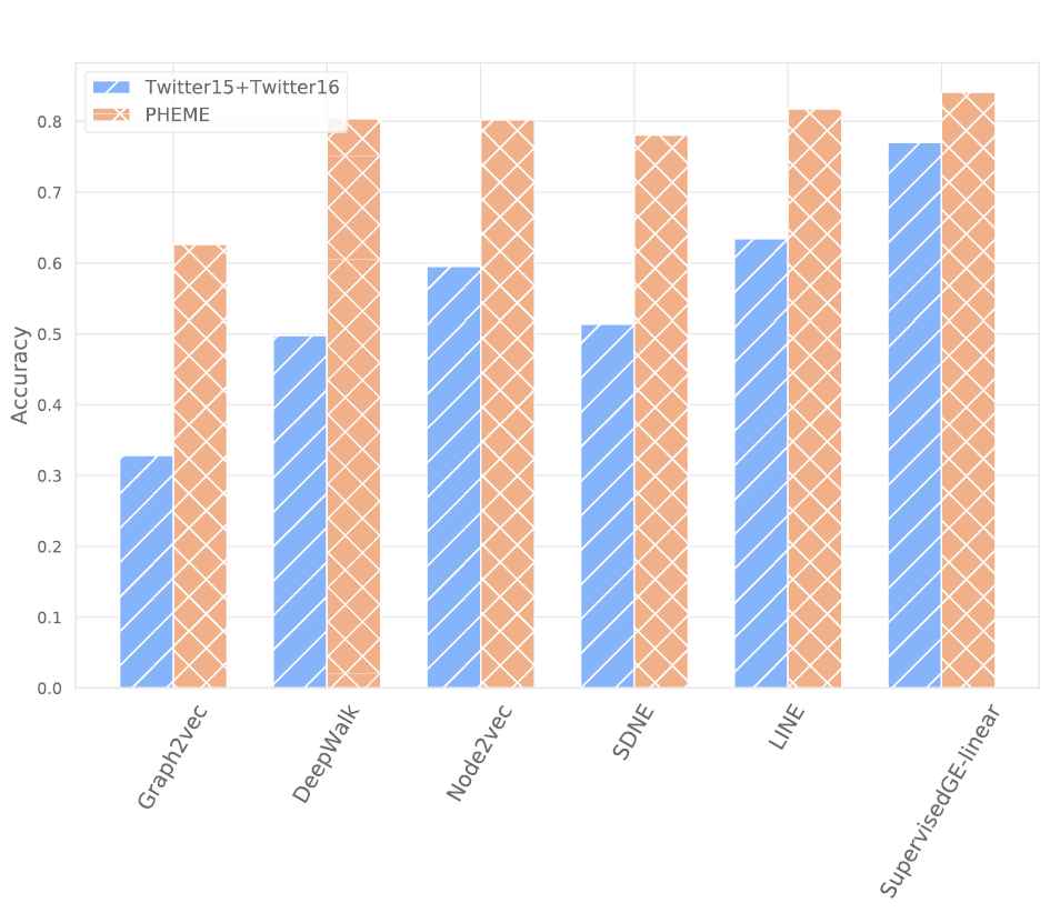
Comparison of graph embedding methods for rumor detection.
6. CONCLUSION AND FUTURE WORK
We have introduced a novel approach to embed whole propagation process of an inspecting post to resolve the rumor detection problem in social networks. Our idea is based on using a graph to model the propagation process: each post is a node, and the relationship between two posts is an edge. Next, we apply different aggregator functions to aggregate neighbor features with node features to output a node embedding vector. Then, we apply a sequence-to-sequence model to learn a representation vector from the sequence of node embeddings. Finally, we classify the representation vector by using a fully connected neural network. Our experiments on Twitter datasets demonstrate that the proposed model outperforms the baseline models as well as recent state-of-the-art models in terms of accuracy, macro-F1, and F1 score of nonrumors and all rumor types.
The advantage of the proposed method is that it efficiently integrates features of the source post and response posts in the propagation process. The combined features will provide valuable information to train a classification algorithm for classifying source posts. However, this method has a disadvantage because it requires data in the whole propagation process of a post to detect rumors. In some cases, if we cannot obtain response posts in the propagation process of a post, the proposed model's accuracy can be reduced. Generally, in this study, we found that i) the propagation structure provides useful features to distinguish between rumor types, ii) the graph embedding method based on a GCN efficiently integrates between content features, social features, temporal features, and propagation structure, iii) the proposed linear aggregator function improves the results of graph embedding by considering the importance of each post in the propagation process. Overall, by efficiently combining features of a post and its response posts, we can improve the accuracy of the rumor detection method.
In our future plan, we intend to build a completely unsupervised model to leverage a large amount of unlabeled social media data. We also plan to find a better method to incorporate the propagation structure with the post features and explore more powerful features to boost the performance of the model. In addition, the existing rumor datasets are relatively small in size, and are not general enough, considering the diversity of information in rumor posts in social networks. This can lead to the overfitting problem of many rumor detection models. Therefore, we intend to build a more diverse dataset to contribute to the development of this research field.
CONFLICTS OF INTEREST
The authors declare no conflict of interest.
AUTHORS’ CONTRIBUTION
Conceptualization, Jason J. Jung; methodology, Jason J. Jung and Dang Thinh Vu; formal analysis, Dang Thinh Vu; writing-original draft preparation, Dang Thinh Vu; writing-review and editing, Jason J. Jung and Dang Thinh Vu; supervision, Jason J. Jung; funding acquisition, Jason J. Jung. All authors have read and agreed to the published version of the manuscript.
ACKNOWLEDGMENTS
This research was supported by the Chung-Ang University Young Scientist Scholarship (CAYSS) Program 2019, and the National Research Foundation of Korea (NRF) grant funded by the Korea government (MSIP) (NRF-2018K1A3A1A09078981, NRF-2020R1A2B5B01002207).
Footnotes
REFERENCES
Cite this article
TY  - JOUR
AU  - Dang Thinh Vu
AU  - Jason J. Jung
PY  - 2021
DA  - 2021/03/16
TI  - Rumor Detection by Propagation Embedding Based on Graph Convolutional Network
JO  - International Journal of Computational Intelligence Systems
SP  - 1053
EP  - 1065
VL  - 14
IS  - 1
SN  - 1875-6883
UR  - https://doi.org/10.2991/ijcis.d.210304.002
DO  - 10.2991/ijcis.d.210304.002
ID  - Vu2021
ER  -