
Slime Mould Algorithm-Based Tuning of Cost-Effective Fuzzy Controllers for Servo Systems
 , Radu-Codrut David1, , Raul-Cristian Roman1, , Emil M. Petriu2, , Alexandra-Iulia Szedlak-Stinean1,
 - DOI
- 10.2991/ijcis.d.210309.001How to use a DOI?
- Keywords
- Low-cost fuzzy control; Optimal tuning; Position control; Servo systems; Slime Mould Algorithm
- Abstract
This paper suggests five new contributions with respect to the state-of-the-art. First, the optimal tuning of cost-effective fuzzy controllers represented by Takagi–Sugeno–Kang proportional-integral fuzzy controllers (TSK PI-FCs) is carried out using a fresh metaheuristic algorithm, namely the Slime Mould Algorithm (SMA), and a fuzzy controller tuning approach is offered. Second, a relatively easily understandable formulation of SMA is offered. Third, a real-world application of SMA is given, focusing on the optimal tuning of TSK PI-FCs for nonlinear servo systems in terms of optimization problems that target the minimization of discrete-time cost functions defined as the sum of time multiplied by squared control error. Fourth, using the concept of improving the performance of metaheuristic algorithms with information feedback models, proposed by Wang and Tan, Improving metaheuristic algorithms with information feedback models, IEEE Trans. Cybern. 49 (2019), 542–555, Gu and Wang, Improving NSGA-III algorithms with information feedback models for large-scale many-objective optimization, Fut. Gen. Comput. Syst. 107 (2020), 49–69, and Zhang et al., Enhancing MOEA/D with information feedback models for large-scale many-objective optimization, Inf. Sci. 522 (2020), 1–16, new metaheuristic algorithms are introduced in terms of inserting the model F1 in SMA and other representative algorithms, namely Gravitational Search Algorithm (GSA), Charged System Search (CSS), Grey Wolf Optimizer (GWO) and Whale Optimization Algorithm (WOA). Fifth, the real-time validation of the cost-effective fuzzy controllers and their tuning approach is performed in the framework of angular position control of laboratory servo system. The comparison with other metaheuristic algorithms that solve the same optimization problem for optimal parameter tuning of cost-effective fuzzy controllers suggestively highlights the superiority of SMA. Experimental results are included.
- Copyright
- © 2021 The Authors. Published by Atlantis Press B.V.
- Open Access
- This is an open access article distributed under the CC BY-NC 4.0 license (http://creativecommons.org/licenses/by-nc/4.0/).
1. INTRODUCTION
Nonlinear models characterize the majority of physical systems and industrial processes, inspiring others to develop suitable approaches for the analysis of nonlinear systems. The rapidly increasing research on fuzzy control that copes with nonlinear systems has taken place in recent decades. This is important because fuzzy control is a robust and inexpensive mathematical approach to control highly complex nonlinear or nonanalytical systems in many industrial applications, and can be considered as a relatively simple initial nonlinear and convenient control approach. As shown by Precup et al. [1] and Precup and David [2], respectively, the systematic design and tuning of fuzzy control systems is supported by analyses that include stability, controllability, observability, sensitivity and robustness. The optimal tuning of fuzzy controllers is combined with these analyses. These analyses are viewed in the context of one of the hot research topic in the recent years, namely the development of the improvement of fuzzy systems performance, owing to their extensively growing applications. To improve the performance of fuzzy control systems, type-1 fuzzy control systems were also extended and generalized to type-2 and type-3 ones especially focusing on interval ones in this regard.
Metaheuristic algorithms are successfully applied because they ensure higher performance and require lower computing capacity and time versus deterministic algorithms in several optimization problems. Such challenging optimization problems are those specific to the optimal (parameter) tuning of fuzzy (logic) controllers, where both the process and the controller are nonlinear and deterministic algorithms are not successful. The following metaheuristic algorithms have been applied most recently to the optimal tuning of fuzzy controllers in representative examples: adaptive weight Genetic Algorithm (GA) for gear shifting control [3], GA-based multiobjective optimization for electric vehicle powertrain control [4], GA for hybrid power systems control [5], engines control [6], energy management in hybrid vehicles [7], servo system control [2], wellhead back pressure control systems [8], micro-unmanned helicopter control [9], Particle Swarm Optimization (PSO) algorithm with compensating coefficient of inertia weight factor for filter time constant adaptation in hybrid energy storage systems control [10], set-based PSO algorithm with adaptive weights for optimal path planning of unmanned aerial vehicles [11], PSO algorithm for zinc production [12] and inverted pendulum control [13], hybrid PSO-Artificial Bee Colony algorithm for frequency regulation in microgrids [14], Imperialist Competitive Algorithm for human immunodeficiency control [15], Grey Wolf Optimizer (GWO) algorithms for sun-tracker systems [16] and servo system control [2], PSO, Cuckoo Search and Differential Evolution (DE) for gantry crane systems position control [17], Whale Optimization Algorithm (WOA) for vibration control of steel structures [18], Grasshopper Optimization Algorithm for load frequency control [19], DE for electro-hydraulic servo system control [20], Gravitational Search Algorithm (GSA) and Charged System Search (CSS) for servo system control [2].
Slime Mould Algorithm (SMA) is a fresh metaheuristic algorithm proposed in [21]. It mimics the oscillation mode of slime mould (i.e., the Physarum polycephalum) in nature when producing positive and negative propagation feedback in the path toward the food. Compared to other metaheuristic algorithms, it is proved in [21] that SMA exhibits improved exploratory and exploitation features.
Other popular metaheuristic algorithms with fresh results are hybrid PSO-GA [22] and hybrid GSA-GA [23] for constrained solutions, water cycle [24] and bat [25] algorithms for combinatorial optimization, GWO with hierarchical fuzzy operator [26], hierarchical GA multiobjective optimization of neural networks [27], Cross-Entropy algorithm for manufacturing processes [28], Water Circle algorithm for traveling salesman problem [29], Conflict Monitoring algorithm [30], Jaya optimization algorithm for biped robots [31] and load forecast [32] and Chemical Reaction algorithm for community detection [33].
Some of the most recently proposed metaheuristic algorithms concern both the improvement of other algorithms and the development of new ones. Suggestive approaches are the improvement of Nondominated Sorting Genetic Algorithm-III (NSGA-III) algorithm with adaptive mutation operator and the application of this improved NSGA-III to Big Data tuning [34], the analysis of the behavior of crossover operators in NSGA-III algorithm and the operator improvement such that to work in large-scale optimization [35], the improvement of DE algorithm by a selection mechanism and its application to fuzzy job-shop scheduling problems [36], and population extremal optimization algorithms applied to continuous optimization and nonlinear controller optimal tuning problems [37–39].
An important and general improvement of metaheuristic algorithms in terms of modifying their structure by including information feedback models is proposed and formulated generally by Wang and Tan [40]. Six types of information feedback models are defined in [40], where individuals from previous iterations are selected in either a fixed or random manner and embedded in the update process of the algorithms. A detailed exemplification on PSO is offered in [40], but experimental applications to other representative algorithms are included as well. This concept is included successfully by Gu and Wang in NSGA-III [41] and Zhang et al. in multiobjective evolutionary algorithms based on decomposition in [42], and has a big potential to be incorporated in other algorithms.
The optimal tuning of fuzzy controller can also be seen, discussed and investigated in the more general and generous context of fuzzy modeling. The estimation capability of fuzzy systems depends on their rule parameters and structure of fuzzy sets. Up to now, many learning methods have been developed for optimizing rule parameters, i.e., which belongs to topic of optimal tuning of parameters of fuzzy model structures. Moreover, evolving fuzzy systems are also a popular topic as they also learn and optimally build the structure of fuzzy systems along with their parameters. Also, research is also focused on the tuning rules, which can be extracted such that to adapt the structure of the fuzzy sets, but these approaches usually also require that the output derivative of fuzzy systems to be computed with respect to the parameters which are actually learned and specifically tuned.
This paper is built upon authors’ recent papers on the optimal tuning of Takagi–Sugeno–Kang proportional-integral fuzzy controllers (TSK PI-FCs) [1,2,43–45] applied to servo systems control such that to obtain a reduced parametric sensitivity (with respect to process gain and time constants), and suggests a novel SMA-based tuning approach. The approach is focused on the position control of nonlinear servo systems viewed as controlled processes. SMA is involved in solving a minimization-type optimization problem, which involves a cost function that is equal to the sum of time multiplied by squared control error, representing the discrete-time version of the Integral of Time Multiplied by Squared Error (ITSE) used in continuous-time control.
The paper suggests the following new contributions:
a fuzzy controller tuning approach,
a relatively easily understandable formulation of SMA,
a real-world application of SMA,
using the concept of improving the performance of metaheuristic algorithms with information feedback models [40–42], new metaheuristic algorithms are proposed by inserting the model F1 in SMA and other representative algorithms, namely GSA, CSS, GWO and WOA,
the real-time validation of cost-effective fuzzy controllers and their tuning approach.
These contributions are significant and also advantageous in the context of the state-of-the-art briefly discussed in this section as the superiority of SMA versus other optimization algorithms, namely PSO, GSA, CSS, GWO and WOA, is proved by means a comparison included in the paper. The comparison is supported by experimental results on a real-world application, namely angular position control of nonlinear servo system; real data from authors’ lab is included.
The next sections in the sequel are structured as follows: the optimization problem is defined in Section 2, and the associated models of the process and fuzzy controller are specified. SMA and, based on this algorithm, the new tuning approach that produces optimal TSK PI-FCs are presented in Section 3. Starting with the introduction of the information feedback model F1 in PSO in [40], details on the new metaheuristic algorithms obtained by inserting the information feedback model F1 in GSA, CSS, GWO and WOA are given in Section 4. The tuning approach is validated in Section 5 in terms of offering experimental results and a comparison as well. The conclusions are drawn in Section 6.
2. PROCESS MODELS, CONTROLLER MODELS AND OPTIMIZATION PROBLEM
The control system structure is illustrated in Figure 1. Figure 1 represents an extended version of the block diagram and description of sub-systems given in [46], highlighting that a continuous-time process is controlled (
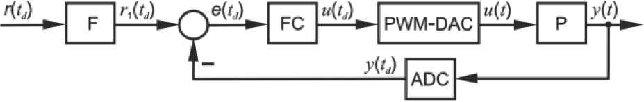
Setpoint filter type two-degree-of-freedom (2-DOF) fuzzy control system structure.
The sub-systems and variables involved in Figure 1 are [46]: F – the setpoint (or the reference input) filter, FC – the fuzzy controller, which is represented by the TSK PI-FC, PWM-DAC – the Pulse Width Modulated (PWM) Digital to Analog Converter that produces the analog voltage applied to the process P (in fact, the actuator), ADC – the Analog to Digital Converter needed for digital process control, r – the reference input, r1 – the reference input filtered through F, y – the controlled output, u – the control signal, and
The servo system that plays the role of P in Figure 1 is characterized by the continuous-time state space model
As shown in [2,44–46], the nonlinearity in (1) is neglected in order to enable the cost-effective linear and nonlinear (including fuzzy) controller design. The transfer function of this simplified model of P, which is next used in the controller design and tuning, is
The servo system process parameters are:
PI controllers are recommended in [47,48] for the process modeled in (2). The transfer function of the PI controller (to be replaced with FC in Figure 1) is
The Extended Symmetrical Optimum (ESO) method suggested in [47,48] is recommended to be applied in order to carried out the PI controller tuning as it guarantees a trade-off to a set of empirical control system quality indices: percent overshoot, settling time, rise time and phase margin. That trade-off is ensured by a single design parameter with the notation β and the recommended domain
The quality of the control system is increased by inserting the cost-effective nonlinear controller represented by TSK PI-FC in terms of the structure given in Figure 1. Incidentally, the design and tuning start with employing the knowledge and experience gained in terms of experimenting PI controllers in various applications. The structure and input membership functions of TSK PI-FC are presented in Figure 2, where [46]: q−1 – the backward shift operator, TISO-FC – the Two Inputs-Single Output Fuzzy Controller sub-system (it is actually a nonlinear sub-system without dynamics as it is introduced outside), e(td) – control error, u(td) – control signal,

Takagi-–Sugeno-–Kang proportional-integral fuzzy controllers (TSK PI-FC) configuration.
The expressions of the two increments illustrated in Figure 2 are obtained by Tustin’s discretization method that leads to the recurrent equation of the incremental discrete-time PI controller
As considered in [47], TISO-FC in Figure 2 uses for defuzzification a weighted average based approach, while the inference engine employs SUM and PROD operators. The rule base of this sub-system consists of only two rules for the sake of cost-effective fuzzy control design and implementation [2,43–46], and it is expressed in Table 1, where the parameter
| N | ZE | P | |
|---|---|---|---|
| P | |||
| ZE | |||
| N |
The parameter η makes the difference in the rule consequents, which consist of two different linear discrete-time PI controllers. This structure of the fuzzy controller makes it behave as a bumpless interpolator between the two linear PI controllers in the rule consequents.
The modal equivalence principle [49] is applied to express one tuning equation for TSK PI-FC
As specified in Section 1, the optimization problem is defined as
3. SMA AND FUZZY CONTROLLER TUNING APPROACH
The operating mechanism of SMA described in accordance with the standard formulation introduced in [21] starts with the random initialization of the population of agents, i.e., agent positions in the slime mould, such that to belong to the search domain Ds. A total number of N agents (i.e., elements of the slime mould) is used, and each agent is assigned to a position vector
The search process specific to SMA continues with approaching, wrapping and grabbling the food. This is modeled by several equations. Using the notation
The vector
The parameters involved in the position update equation are computed in terms of
Using the notation
SMA consists of steps SMA1 to SMA7. These steps are given as follows after the revision of the algorithm presented in [21]:
SMA1. The initial random population, which consists of the position vectors
SMA2. The performance of each element of the population of agents (i.e., the slime mould) is evaluated; this evaluation involves simulations and/or experiments conducted on the fuzzy control systems if the optimal tuning of fuzzy controllers is carried out. The evaluation leads to the fitness function values of all agents.
SMA3. The best fitness
SMA4. The vector
SMA5. Agents’ positions are updated using (25), which is supported by (21)–(24), (26) and (27).
SMA6. The iteration index k is incremented with one. The algorithm goes on with step 2 until
SMA7. The solution to the optimization problem is the last best agent obtained so far, i.e., the vector
SMA is used in the optimization problem defined in (11) in terms of the following relationships:
Using the aspects presented in this section and the previous one, the SMA-based tuning approach dedicated to TSK PI-FCs consists of proceeding the steps 1–4. These steps are briefly described as follows:
Step 1. As pointed out in [46], the sampling period Ts is set in accordance with the requirements of quasi-continuous digital control.
Step 2. The feasible domain Dρ is set in order to include all constraints imposed to the elements of ρ.
Step 3. SMA is integrated using steps SMA1 to SMA7 and (28) in solving the optimization problem defined in (11) leading to the optimal parameter vector ρ* in (12) and three of the optimal parameters of TSK PI-FC, namely
Step 4. The optimal parameter
4. INSERTING INFORMATION FEEDBACK MODEL F1 IN METAHEURISTIC ALGORITHMS
Using the notation in (13) for the position vector
Equations (30) and (31) are successfully integrated in PSO algorithms [40], in NSGA-III algorithms [41], and in multiobjective evolutionary algorithms based on decomposition [42]. The agent (or particle) velocity and position update equations employed in PSO algorithms are [2]
The position and velocity updates in GSA are governed by the recurrent equations [2]
The new position and velocity vectors of ith agent (or charged particle) in CSS algorithms are calculated in terms of [2]
The updated agent (i.e., grey wolf) position vector in GWO algorithms is obtained in terms of [2]
The GWO algorithm with information feedback model F1 will be referred to as GWO-F1 algorithm.
Using the notation Xbest(k) for the best agents’ position (i.e., the position of the prey tracked by the whales, which are the agents) vector in the population at iteration k, the position update equation in WOA is [45]
5. VALIDATION AND COMPARISON
SMA with information feedback model F1 (SMA-F1) and the tuning approach presented in Section 3 are validated in this section by the optimal tuning of TSK PI-FCs for the angular position control of the experimental setup described in [56], which belongs to the Intelligent Control Systems Laboratory of the Politehnica University of Timisoara, Romania. A photo of the experimental setup is given in Figure 3. The parameter values of the servo system models given in (1) and (2) are
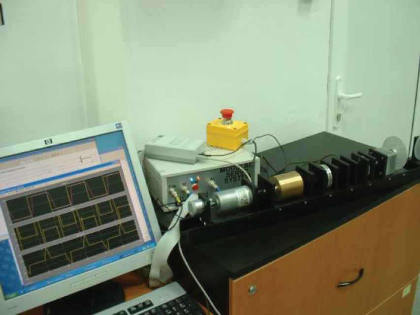
Experimental setup.
The sampling period was set to
The dynamic regimes considered in the optimization problem are characterized by the
The parameters of SMA were set in step 3 using the recommendations given in [21], namely
The simulations and experiments were run in Matlab R2007b environment on a personal computer with Windows 10 operating system and the following hardware configuration: CPU Intel Core i5-7500, 3.4 GHz quad-core, 16 GB of DDR3 RAM memory at 1600 MHz, 256 SSD. These details are convenient for other researchers to redo the experiments, thus making the work in this paper relatively easily acceptable.
The optimal controller parameters and the corresponding minimum cost function Jmin in relation with (11) are presented in Table 2. Table 2 includes suggestively the comparison with other metaheuristic algorithms, namely PSO, GSA, CSS, GWO, WOA, PSO with information feedback model F1 (PSO-F1), GSA with information feedback model F1 (GSA-F1), CSS with information feedback model F1 (CSS-F1), GWO with information feedback model F1 (GWO-F1) and WOA with information feedback model F1 (WOA-F1). The same numbers of agents
|
Algorithm |
|||||||
|---|---|---|---|---|---|---|---|
| SMA | 38 | 0.75 | 0.00857633 | 4.821519 | 0.0035384 | 4.435799 | 2797210 |
| PSO | 36.5966 | 0.5935440 | 0.0819451 | 4.913505 | 0.00352454 | 4.520424 | 3523353 |
| GSA | 33.0287 | 0.7414017 | 0.0786853 | 4.770794 | 0.00360137 | 4.398443 | 3693850 |
| CSS | 23.1039 | 0.6662344 | 0.0715622 | 3.776415 | 0.00407048 | 3.4743 | 4935620 |
| GWO | 37.9457 | 0.6994276 | 0.0857001 | 4.910214 | 0.00352702 | 4.517395 | 3315304 |
| WOA | 35.0330 | 0.6513980 | 0.0748931 | 5.09787 | 0.0034414 | 4.682604 | 3297086 |
| SMA-F1 | 38 | 0.75 | 0.0857638 | 4.821494 | 0.00353585 | 4.435774 | 2797210 |
| PSO-F1 | 27.5769 | 0.6315154 | 0.0601471 | 5.161258 | 0.00341579 | 4.748359 | 3905199 |
| GSA-F1 | 32.6942 | 0.7219313 | 0.0685116 | 5.194281 | 0.00340791 | 4.778737 | 3444169 |
| CSS-F1 | 20.8791 | 0.7095039 | 0.0464305 | 4.962937 | 0.00351122 | 4.565903 | 4213287 |
| GWO-F1 | 34.9617 | 0.7367405 | 0.0770037 | 4.030243 | 0.00350845 | 4.550747 | 3355471 |
| WOA-F1 | 34.2792 | 0.6915126 | 0.1020510 | 3.799553 | 0.00407587 | 3.495585 | 5236392 |
CSS, Charged System Search; CSS-F1, Charged System Search with information feedback model F1; GSA, Gravitational Search Algorithm; GSA-F1, Gravitational Search Algorithm with information feedback model F1; GWO, Grey Wolf Optimizer; GWO-F1, Grey Wolf Optimizer with information feedback model F1; PSO, Particle Swarm Optimization; PSO-F1, Particle Swarm Optimization with information feedback model F1; SMA, Slime Mould Algorithm; SMA-F1, Slime Mould Algorithm with information feedback model F1; WOA, Whale Optimization Algorithm; WOA-F1, Whale Optimization Algorithm with information feedback model F1.
The performance of SMA and other algorithms considered in Table 2 was assessed using two quality indices. The first index reflects the convergence speed cs by measuring the number of evaluations required for the cost function J(ρ) until obtaining the optimal solution ρ*. The second index reflects the accuracy rate ar defined as the percent value of standard deviation of J(ρ) obtained by running a certain metaheuristic algorithm divided to the average value of the solution,
The search performance of all metaheuristic algorithms analyzed in this section is synthesized in Table 3 in terms of the values of the quality indices cs and ar.
The results presented in Table 2 indicate that the best performance of the control system as far as the average value of the cost function is concerned is obtained by SMA and SMA-F1 followed by WOA, and the worse performance is obtained by CSS and WOA-F1. The comparison of accuracy and resource usage on the basis of the results given in Table 3 reveals that the best accuracy rate is obtained by SMA and SMA-F1 followed by WOA, and the worse is obtained by GSA and GWO-F1. The best convergence speed is obtained by SMA-F1 followed by SMA-F1 and GWO, and the worse by PSO-F1 and PSO. Concluding, the best overall performance is exhibited by SMA and SMA-F1, which is followed by WOA, justifying the application of SMA in this paper.
| Algorithm | cs | ar |
|---|---|---|
| SMA | 19.7 | 0 |
| PSO | 311.4 | 18.67 |
| GSA | 167.2 | 18.86 |
| CSS | 97.9 | 12.07 |
| GWO | 20 | 18.52 |
| WOA | 18.7 | 6.24 |
| SMA-F1 | 14.3 | 0 |
| PSO-F1 | 269.9 | 11.77 |
| GSA-F1 | 204.4 | 12.82 |
| CSS-F1 | 162.9 | 11.33 |
| GWO-F1 | 180.4 | 20.49 |
| WOA-F1 | 11.9 | 14.9 |
CSS, Charged System Search; CSS-F1, Charged System Search with information feedback model F1; GSA, Gravitational Search Algorithm; GSA-F1, Gravitational Search Algorithm with information feedback model F1; GWO, Grey Wolf Optimizer; GWO-F1, Grey Wolf Optimizer with information feedback model F1; PSO, Particle Swarm Optimization; PSO-F1, Particle Swarm Optimization with information feedback model F1; SMA, Slime Mould Algorithm; SMA-F1, Slime Mould Algorithm with information feedback model F1; WOA, Whale Optimization Algorithm; WOA-F1, Whale Optimization Algorithm with information feedback model F1.
The results presented in Table 2 show that adding the information feedback model F1 is beneficial for SMA, GSA and CSS as far as the reduction of cost function values is concerned. The results presented in Table 3 highlight that adding the information feedback model F1 offers the reduction of the convergence speed of SMA, PSO and WOA. But the main advantage of adding the information feedback model, as outlined in Table 3, is the reduction of the accuracy rate of all algorithms except GSO and WOA.
These conclusions are drawn for the process, fuzzy controller, optimization problem and dynamic regime considered in this paper. Other processes, controllers, optimization problems and dynamic regimes are expected to lead to different conclusions; challenging processes in this regard are those considered in [57–64].
Two typical fuzzy control system responses are presented in Figure 4 in terms of controlled output and control signal versus time considering the average controller after the first iteration of SMA (with the parameters

Real-time experimental results expressed as fuzzy control system responses y and u with Takagi–Sugeno–Kang proportional-integral fuzzy controllers (TSK PI-FC) after one iteration of Slime Mould Algorithm (SMA) (dotted line) and after 20 iterations of SMA (continuous line).
It is certainly obvious from Figure 4 that the output trajectories blend to reference input value as time approaches the end of the time horizon. As a consequence, with the suggested controller, the control system addressed can be stabilized. However, as pointed out in [44], the stability cannot be proved.
6. CONCLUSIONS
This paper proposed an approach to the SMA-based tuning of cost-effective fuzzy controllers for servo systems. This approach is advantageous because of two reasons, (1) and (2), which represent the pros of the approach proposed in this paper in the framework of metaheuristic optimization algorithms: (1) it is computational efficient as proved by the values of two quality indices related to accuracy and resource usage, (2) SMA has a small number of parameters. The validation and comparison on real-world servo system position control shows the superior performance of SMA versus other similar metaheuristic algorithms reflected by smaller value of the cost function, defined, as specified in Section 1, as the sum of time multiplied by squared control error, which is the discrete-time version of ITSE used in continuous-time control.
The limitations of SMA, which are also the cons of the approach proposed in this paper, are also twofold, (i) and (ii): its current implementation is offline, (ii) it requires a relatively large number of evaluations of the cost function (or the fitness function). But these two cons are also met at other metaheuristic algorithms.
Future research will be focused on the mitigation of these limitations by modifying SMA in order to work online in adaptive fuzzy control system structure, and solving other optimization problems including those specific to optimal tuning of controller parameters in optimization problems expressed as reference tracking control problems.
Moreover, except the algorithms used in this paper, some of the most representative computational intelligence algorithms can be used to solve the problems, like Monarch Butterfly Optimization (MBO) [65], Earthworm Optimization Algorithm (EWA) [66], Elephant Herding Optimization (EHO) [67] and Moth Search (MS) algorithm [68]. Another group of representative algorithms is discussed in [69].
Nevertheless, a viable way to apply the results given in this paper is represented by networked control systems. With the increasing progress in advanced data communication technology, sampled-based event-triggered control protocols have been introduced in such systems and especially in complex networked control systems to effectively alleviate the communication burden by reducing computation loads and data transmission rates. Therefore this motivates the attempt to further enhance the performance of such control systems in terms of using fuzzy control, and the optimal tuning of tuning parameters is a convenient way to cope with such systems.
CONFLICT OF INTEREST
The authors declare that they do not have any conflict of interest.
AUTHOR’S CONTRIBUTION
The contribution of the authors to this paper is equal.
ACKNOWLEDGMENTS
This work was supported by grants of the Romanian Ministry of Education and Research, CNCS - UEFISCDI, project numbers PN-III-P4-ID-PCE-2020-0269, PN-III-P1-1.1-PD-2019-0637, PNIII-P1-1.1-PD-2016-0331, PN-III-P1-1.1-TE-2019-1117, PN-III-P2-2.1-PTE-2019-0694, within PNCDI III, and by the NSERC of Canada.
REFERENCES
Cite this article
TY  - JOUR
AU  - Radu-Emil Precup
AU  - Radu-Codrut David
AU  - Raul-Cristian Roman
AU  - Emil M. Petriu
AU  - Alexandra-Iulia Szedlak-Stinean
PY  - 2021
DA  - 2021/03/16
TI  - Slime Mould Algorithm-Based Tuning of Cost-Effective Fuzzy Controllers for Servo Systems
JO  - International Journal of Computational Intelligence Systems
SP  - 1042
EP  - 1052
VL  - 14
IS  - 1
SN  - 1875-6883
UR  - https://doi.org/10.2991/ijcis.d.210309.001
DO  - 10.2991/ijcis.d.210309.001
ID  - Precup2021
ER  -