
Optimal FOC-PID Parameters of BLDC Motor System Control Using Parallel PM-PSO Optimization Technique

- DOI
- 10.2991/ijcis.d.210319.001How to use a DOI?
- Keywords
- Particle swarm optimization (PSO); Parallel PSO technique; Parallel multi-population technique; Brushless DC electric motor; BLDC motor system; Field-oriented control (FOC-PID); Nonlinear Benchmark tests; Parallel multi-population particle swarm optimization (PM-PSO)
- Abstract
This paper proposes a parallelization method for meta-heuristic particle swarm optimization algorithm to obtain a convincingly fast execution and stable global solution result. Applied the proposed method, the searching region is efficiently separated into sub-regions which are simultaneously searched using optimization algorithm. The structure of meta-heuristic algorithm is rebuilt as to execute in parallel multi-population mode. The closed loop system of brushless DC electric motor position control is used to verify the proposed method. The simulation and experiment results show that the proposed parallel multi-population technique obtains a competitive performance compared to the standard ones in both of precision and stability criteria. Especially, meta-heuristic algorithms running in parallel multi-population mode execute quite faster than standard ones. In particular, it shows an efficient improvement of the proposed method applied to identify of nonlinear Benchmark tests and to optimize proportional integral derivative parameters for field-oriented control scheme of the brushless DC electric motor system.
- Copyright
- © 2021 The Authors. Published by Atlantis Press B.V.
- Open Access
- This is an open access article distributed under the CC BY-NC 4.0 license (http://creativecommons.org/licenses/by-nc/4.0/).
ACRONYMS
| BLDC | Brushless DC Electric Motor |
| FOC | Field-Oriented Control |
| PID | Proportional Integral Derivative |
| PSO | Particle Swarm Optimization |
| SPSO | Standard Particle Swarm Optimization |
| PM-PSO | Parallel Multi-Population Particle Swarm Optimization |
1. INTRODUCTION
Particle swarm optimization (PSO) algorithm introduced by Eberhart and Kennedy [1,2] is a powerful basic algorithm for resolving different types of optimization applications. Its principle relies on the social-sharing information among particles aim to reach an evolutionary benefit. Thus those algorithms have been widely used in searching for the best optimum solution within a specified range in which random population is created.
Recently, many research related to PSO algorithms have been applied in various areas such as optimal problem [3], modification of landslide susceptibility mapping [4], estimating α ratio in driven piles [5], path planning [6], color image segmentation [7]. Regarding to brushless DC electric motor (BLDC) motor control there have been several advanced control techniques, such as optimal control, nonlinear control, and adaptive control, being applied for velocity and position control of BLDC [8,9]. Three elements of proportional integral derivative (PID) block can efficiently handle both of transient and steady control stages and then shows a simple but effective solution to numerous control tasks. Nevertheless, optimal updated PID parameters seem really hard. Recently evolutionary optimization algorithms, such as PSO, have been improved it in many ways to solve optimal problem [10–13]. Moreover, it is interested in applying PSO in tuning, optimizatio,n and identification BLDC motor. Those researches show that the PSO can solve lots of optimized problems, but it takes a lot of time to find out the best solution [14–19].
Development of big data technologies have also initiated the generation of complex optimization problems with large size. The high calculation cost of these problems has accounted for the development of optimization algorithms with parallelization. PSO algorithm is one of the most popular swarm intelligence-based algorithms, which shows its robustness, simplicity, and global search proficiency. However, one of the major PSO obstacles is frequency of getting entrapped in local optima and being deteriorated as soon as the dimension of the problem increases. Hence, numerous efforts are made to reinforce its performance that includes the parallelization of PSO. The basic architecture of PSO inherits a natural parallelism, and receptiveness of fast processing machines has made this task pretty convenient. Therefore, parallelized PSO (PPSO) has emerged as a well-accepted algorithm by the research community. Several studies have been performed on parallelizing PSO algorithm so far [20–26]. To investigate and model the batch culture of glycerol to 1,3-propanediol, Yuan et al. [21] presented nonlinear switched system which is enzyme-catalytic, time-delayed and contains switching times, unknown state delays, and system parameters. The process contains state inequality constraints and parameter constraints accompanied by calibrated biological robustness as a cost function. To extract and estimate the parameters of the PV cell model, Ting et al. [22] proposed parallel swarm algorithm (PSA) that minimizes root-mean-square error that seeks the difference between determined and computed current value. They coded the fitness functions in OpenCL kernel and executed it on multi-core CPU and GPUs. Further, Liao et al. [23] proposed multi-core PPSO (MPPSO) for improving the computational efficiency of system operations of long-term optimal hydropower for solving the issue of speedily growing size and complexity of hydropower systems. The algorithm claims to achieve high-quality schedules for pertinent operations of the hydropower system. Li et al. [24] used parallel multi-population PSO with a constriction factor (PPSO) algorithm to optimize the design for the excavator working device. They authenticated kinetic and dynamic analysis models for the hydraulic excavator. Luu et al. [25] proposed a competitive PSO (CPSO) to improve algorithm performance with respect to stagnation problem and diversity. Arqub et al. [27,28] introduced the continuous genetic algorithm (GA) as a solver for boundary value problem of second-order systems and also proposed a new approach of fuzzy fractional derivative which is efficient and conformable to solve numerical solution.
Improved from above referred applications of PSO, this paper proposed the method splitting searching region into pieces of sub-region, in which the independent sub-population is created, aimed to greatly reduce computing time. This result is ameliorated in utilizing the power of multi-core processor through which all sub-regions of PSO structure are simultaneously searching by sub-population. Consequently, a best vector that contains global best stage of each sub-population is returned and the global best solution of main-population is successfully selected. Recently, new types of hardware that deliver massive numbers of parallel processing power so running parallel multi-population is possible. Moreover, recent CPU architectures have significant modifications leading to high-performance computing capabilities. One of those high-performance computing capabilities is Parallel Computing Toolbox that can solve intensive computing and data problems using multi-core processors. High-level constructions, such as parallel for loops, special types of arrays and parallelized digital algorithms, are supported. The toolbox allows programmer to use the functions supporting parallel calculation with MATLAB and other toolboxes. It is possible to use the toolbox with Simulink® to run several simulations of a model in parallel. The toolbox allows you to use all the processing power of multi-core computers by running applications on workers (MATLAB computing engines) that run locally so each sub-population can be setting up independently on each available worker. So, parallel multi-population PM-PSO algorithm is innovatively proposed for optimizing the PID parameters of BLDC controller. It shows the competitive performance compared to the standard ones.
The rest of this paper is structured as follows. Section 2 introduced the implementation of FOC algorithm to control BLDC motor system using MATLAB/Simulink platform. Section 3 presents the standard SPSO algorithm used to optimize PID parameters of BLDC FOC control. Section 4 presents the newly proposed parallel multi-population PM-PSO technique. Simulation and experiment results of proposed algorithm applied in four Benchmark tests and used to optimize PID parameters of BLDC FOC position control are fully presented in Section 5. Eventually Section 6 includes the conclusions.
2. BLDC FOC CONTROL ALGORITHM
The advantage of BLDC motors is not use mechanical components and brushes to commutate, in which the stator represents the coil and rotor includes permanent magnets. In this research, a 2-pole BLDC will be investigated, through which not only gathers the benefits of DC machine for example better speed ability with not mechanical commutator but includes the superiority of AC motor related to simple, high reliable, and no-maintenance. Furthermore, BLDC also possesses followed benefits: compact volume and powerful torque. Then it is often used in applications required highly driving quality. The FOC algorithm is applied to control a 3-phase synchronous motor in the dq0 domain. The advantage of this method is that it can simultaneously control the angle-speed and torque of the BLDC. The main structure of the FOC control algorithm can be divided into two main control layers. The first control layer is used to control two values d and q in order to generate the vector of Stator magnetic as desired. Meanwhile, the 2nd control layer is used to control the angular depend on controlling q value as presented in Figure 1.
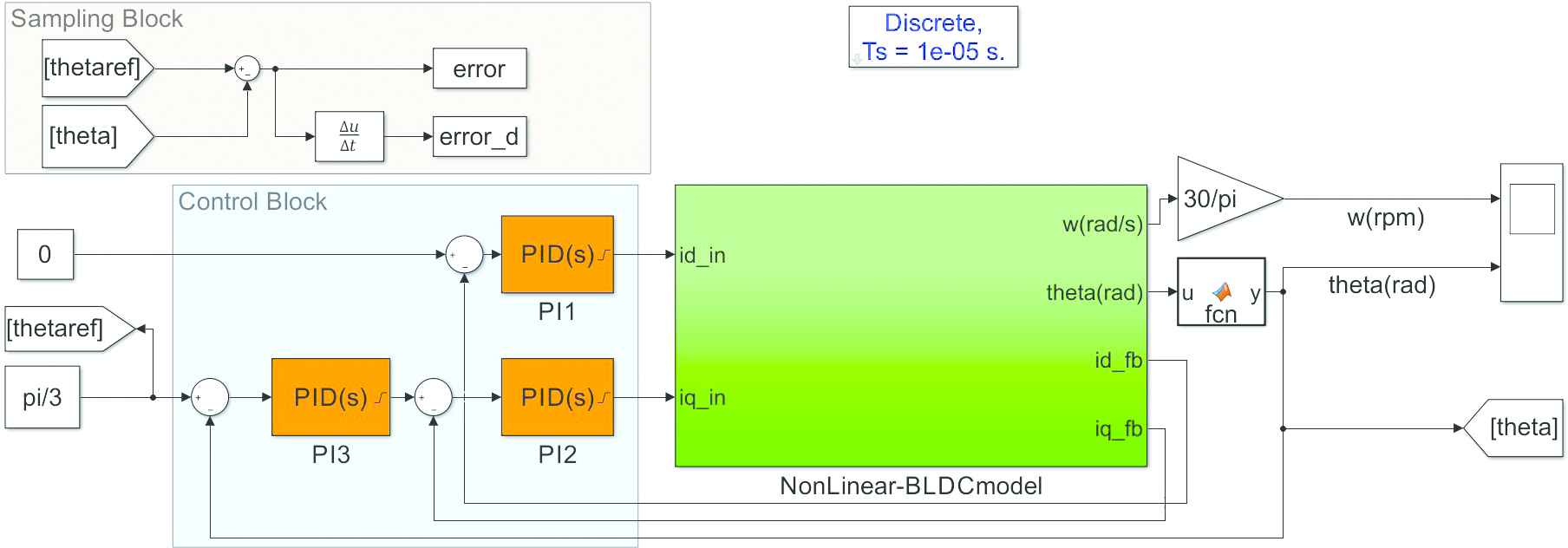
The standard field-oriented control (FOC) scheme.
Figure 2 shows that the BLDC rotor angle value is determined by using location sensor. The values
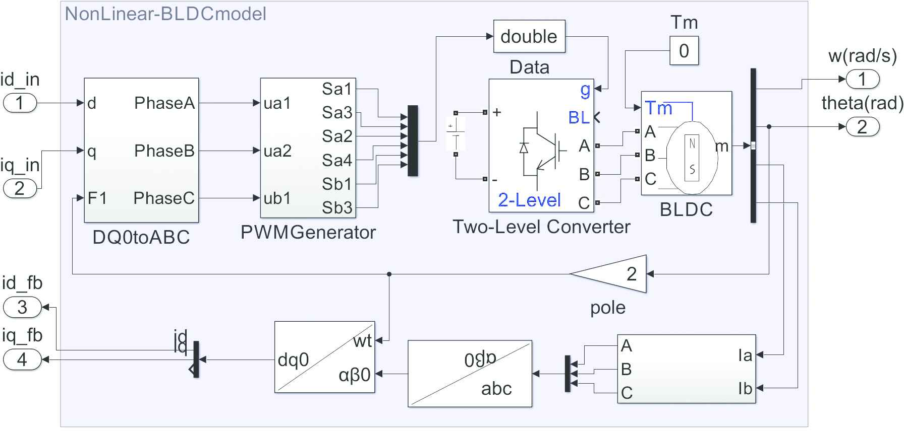
The 3-phase full-bridge scheme for brushless DC electric motor (BLDC) position control.
The important parameters of BLDC control system are chosen as follows:
| LqLd | H | 8.5e-3 | J | kg.m2 | 0.0008 | |
| R | Ohm | 2.87 | F | N | 1.349e-05 | |
| V.s | 0.175 | Tf | N.m | 0 | ||
| P | 2 |
To simulate this control model, we need to perform the following below steps. In Simulink blocks of MATLAB, select the block “Permanent Magnet Synchronous Motor” with Trapezoidal Back-EMF waveform presented in Figure 3.
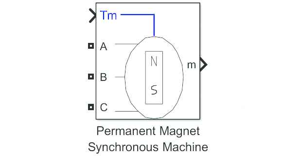
Brushless DC electric motor (BLDC) Simulink block.
The mathematical model formulas (1–5) are presented for the nonlinear BLDC simulation model shown in Figure 2:
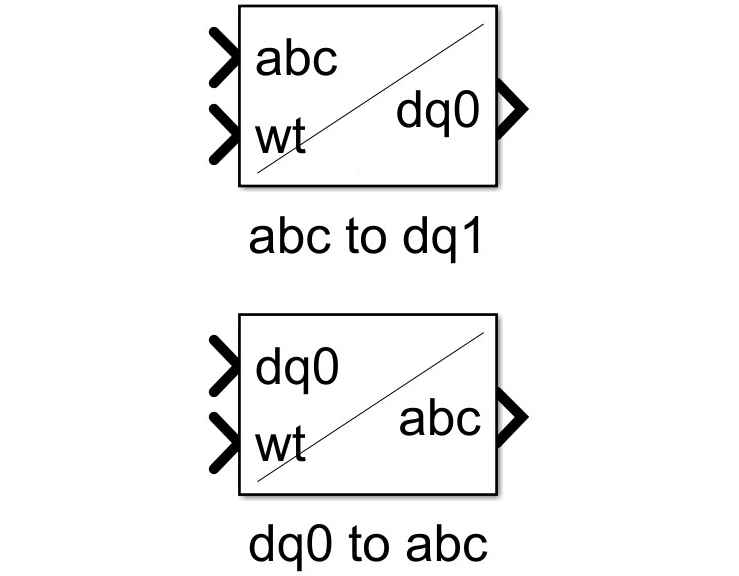
The main control blocks are shown in Figure 1. The BLDC control system consist of transforming dq to abc block, SPWM block, Encoder signal transforming block and PI block used to control BLDC system.
“
“
The transformations of “
PID control schemes are now widely applied in numerous industrial control processes. It is important to note that the PID scheme is easy to be performed badly and even becoming unstable in case inappropriate values of PID controller which were chosen. Thus the fact is that it is crucially necessary to tune the PID coefficients to obtain the best performance within the bounded range.
The three coefficients of PID block must be carefully selected as to satisfy preset quality requirements, with respect to rising and steady time, overshoot percentage, etc. In this study parallel multi-population PM-PSO algorithm is innovatively applied to optimally identify the optimum coefficients of three PI control block for BLDC FOC-PID position control scheme.
3. OPTIMIZING FOC-PID PARAMETER BASED ON STANDARD PSO ALGORITHM
The standard PSO algorithm initializes a random population of solutions. At each generation, all of fitness function values are calculated to determine best value of those members in this population. In standard PSO, the member of population, called particle, move within a n-dimension of searching region with a velocity that is automatically adjusted base on its own experience and sharing information of its neighbors.
In standard PSO algorithm, a population included NP member are created for searching best stage within main searching range called
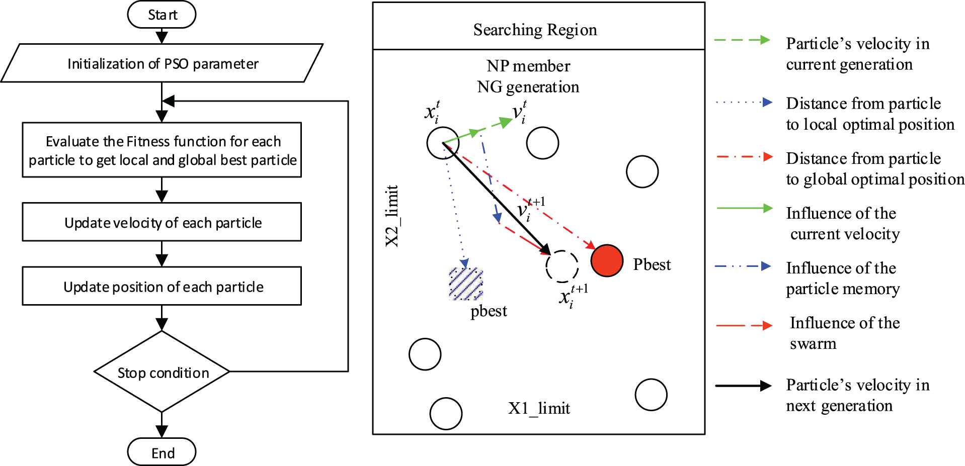
Flow-chart of standard particle swarm optimization (PSO).
In which
The PSO approach is used to optimally identify the parameters for PID block. This procedure can guide the swarm's particles shift to space with fitness value more available and eventually reach the global optimum solution. In Standard PSO method, each particle contains six members as
Using (8) and (9), particle's speed eventually moves to pbest and Pbest, will be updated each step in processing iteration with its current location is updated using (9) as figured in Figure 5.
In this case, fitness function is determined as
Fitness function J with
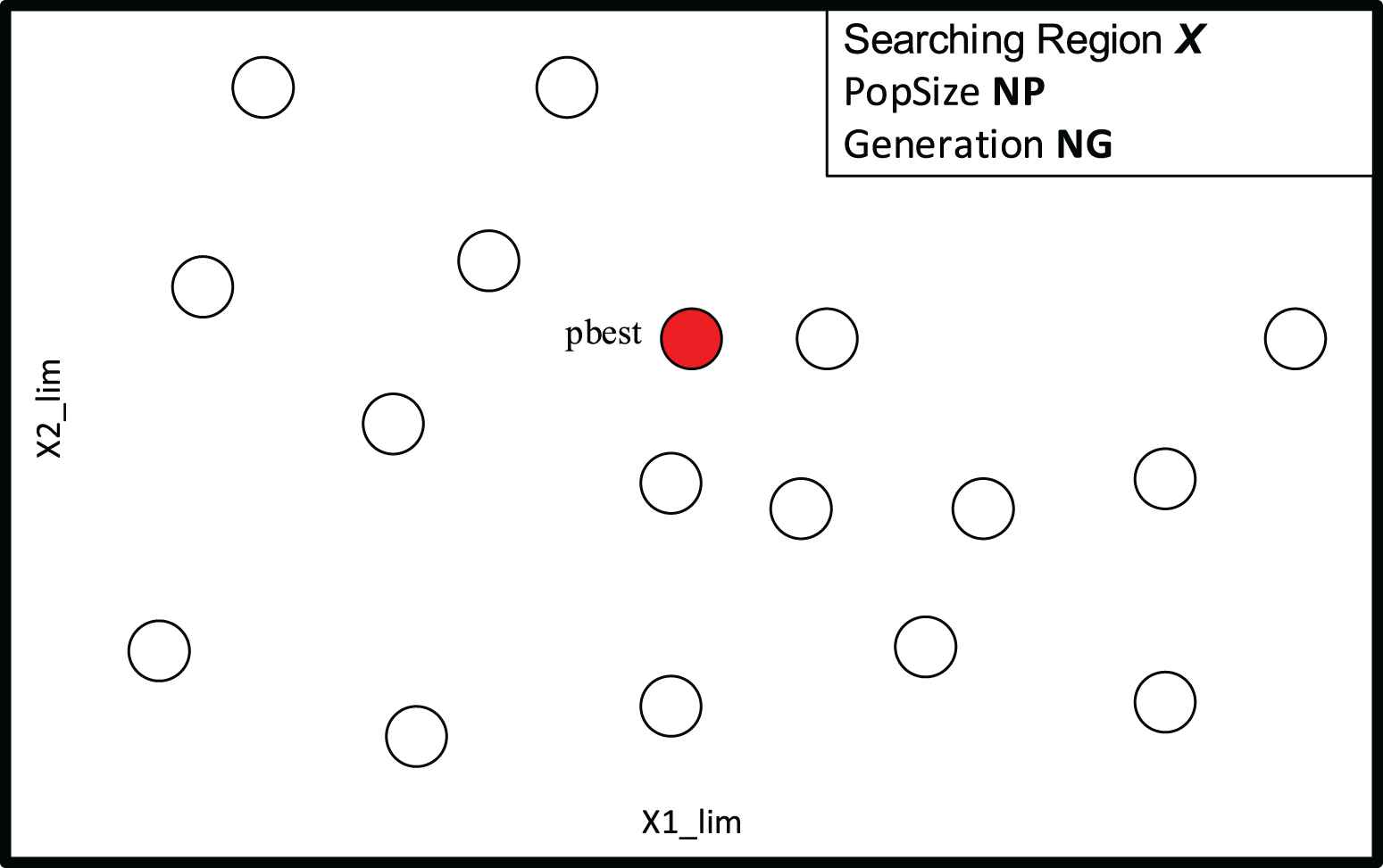
Principle of standard particle swarm optimization (SPSO) executed on single core.
4. PROPOSED PARALLEL MULTI-POPULATION TECHNIQUE APPLIED ON PM-PSO ALGORITHM
This paper proposes the parallel multi population technique called PM technique, the searching region is split into many sub-searching region according to classified parameter such as
Firstly, the searching region is separated into
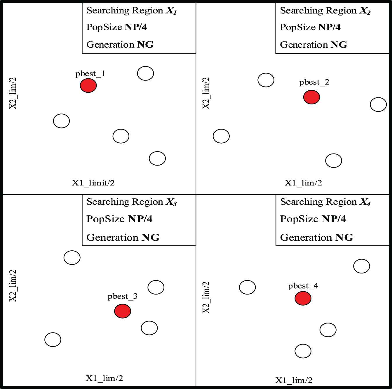
Principle of parallel multi-population technique executed on multi cores.
The parallel multi-population technique expected to perform for fast execution and stable results of PMPSO optimization algorithms. Firstly, splitting up searching region decreased local extremes rate of the results because there is
The performance and effectiveness of parallel multi-population are tested on four benchmark-test functions detailed below in Subsection 5.1. Then, it is compared to the standard SPSO algorithm. All experiments are run with Matlab 2016b on the Intel Core i5 8th Gen 1.6 Mhz and 8Gb RAM.
The control parameter of all algorithms used to optimize are listed. It is included inertia weight (
| Case | PSO (Serial Implementation) | PM-PSO (Parallel Implementation) | |||
|---|---|---|---|---|---|
| Case1010 | NG | 10 | 10 | ||
| NP | 24 | 6 × 4 | |||
| No. core | 1 | 4 | |||
| Case1048 | NG | 10 | 10 | ||
| NP | 48 | 12 × 4 | |||
| No. core | 1 | 4 | |||
| Case1060 | NG | 10 | 10 | ||
| NP | 60 | 15 × 4 | |||
| No. core | 1 | 4 | |||
| Case1072 | NG | 10 | 10 | ||
| NP | 72 | 18 × 4 | |||
| No. core | 1 | 4 | |||
| Details of multi-core processor | |||||
| Specification | Intel Core i5 8250U CPU @ 1.60 MHz | ||||
| Cores | 4 | ||||
| Threads | 8 | ||||
PSO, particle swarm optimization.
PSO parameter of each case and parameter of Intel Core i5 computers.
5. RESULTS AND DISSCUSSION
5.1. Four Benchmark Test Functions
The performance and effectiveness of parallel multi-population PMPSO are tested on four benchmark functions detailed below. Then, it is compared to the standard algorithm SPSO. All experiments are simulated by Matlab 2016b on Intel Core i5 8th Gen 1.6 Mhz and 8Gb RAM.
The principal parameters of two optimization algorithms used are listed in Table 2. It is included inertia weight (w), particle's best weight (
| SPSO | PM-PSO | |||
|---|---|---|---|---|
| NP | 50 | 50 | ||
| NG | 2000 | 500 | ||
| 1 | 4 | |||
SPSO, standard particle swarm optimization; PSO, particle swarm optimization
The parameters of SPSO, PM-PSO.
The four benchmark functions used to test the performance and effectiveness of proposed parallel multi-population PM-PSO are described as follows:
Rosen Brock: Valley-Shaped
Global minimum:
Dimension: 10, whereas
Searching region:
Griewank: Many Local Minima
Global minimum:
Dimension: 20, where as
Searching region:
Ackley: Many Local Minima
Global minimum:
Dimension: 20, whereas
Searching region:
Michalewicz: Steep Ridges/Drops
Global minimum:
Dimension: 10, where as
Searching region:
For each Benchmark Test, 50 independent runs are carried out and the statistical results of the best, worst, mean, and standard deviation for four optimization algorithms are shown in Table 3. The bold values show the best value of each case test, which is compared results between classical SPSO and parallel multi-technique PM-PSO, fully presented in the table.
| Function | SPSO | PM-PSO | |
|---|---|---|---|
| Rosenbrock | Best | 4.0068 | 0.0017 |
| Worst | 3.3315e+4 | 78.9591 | |
| Mean | 215.1817 | 7.2705 | |
| StdDev | 556.9688 | 12.0427 | |
| Time (s/run) | 0.2148 | 0.1697 | |
| Griewank | Best | 0.0951 | 0.2916 |
| Worst | 1.2870 | 3.5631 | |
| Mean | 0.7840 | 1.7050 | |
| StdDev | 0.3560 | 0.7924 | |
| Time (s/run) | 0.4165 | 0.1905 | |
| Ackley | Best | 2.7652 | 3.0496 |
| Worst | 10.2113 | 8.8752 | |
| Mean | 5.7396 | 6.3287 | |
| StdDev | 1.5309 | 1.3282 | |
| Time (s/run) | 0.6841 | 0.3033 | |
| Michalewicz | Best | −8.7674 | −9.1561 |
| Worst | −4.2685 | −5.7805 | |
| Mean | −6.3755 | −7.3387 | |
| StdDev | 1.0549 | 0.7246 | |
| Time (s/run) | 0.4733 | 0.1767 |
SPSO, standard particle swarm optimization; PSO, particle swarm optimization
The experiment results of testing benchmark functions.
As can be seen from the results shown in Table 3 and Figure 8, the parallel multi-technique applied on PM-PSO yields superior results compared to the classical ones in running time criteria. It is clear that the running time of the heuristic algorithms applied PM Technique is significantly faster than the classical ones. In detail, Rosenbrock function optimized by PSO take 0.21s per run meanwhile it take 0.17s in PM-PSO technique. Same results as Rosenbrock function, Griewank, Ackley, and Michalewicz tested by classical PSO take 0.42s, 0.68s, and 0.47s worse than approximately three times when running by PM-PSO that is 0.19s, 0.30s, and 0.18s, respectively. Abovementioned principle of both algorithms, PSO have to use two “for loop,” one for calculating all member value and one for moving member after that. As indicated in Figure 8, The parallel multi-technique is strongly improved processing time of classical PSO algorithm and the returned results are completely finer which shown in Table 3.
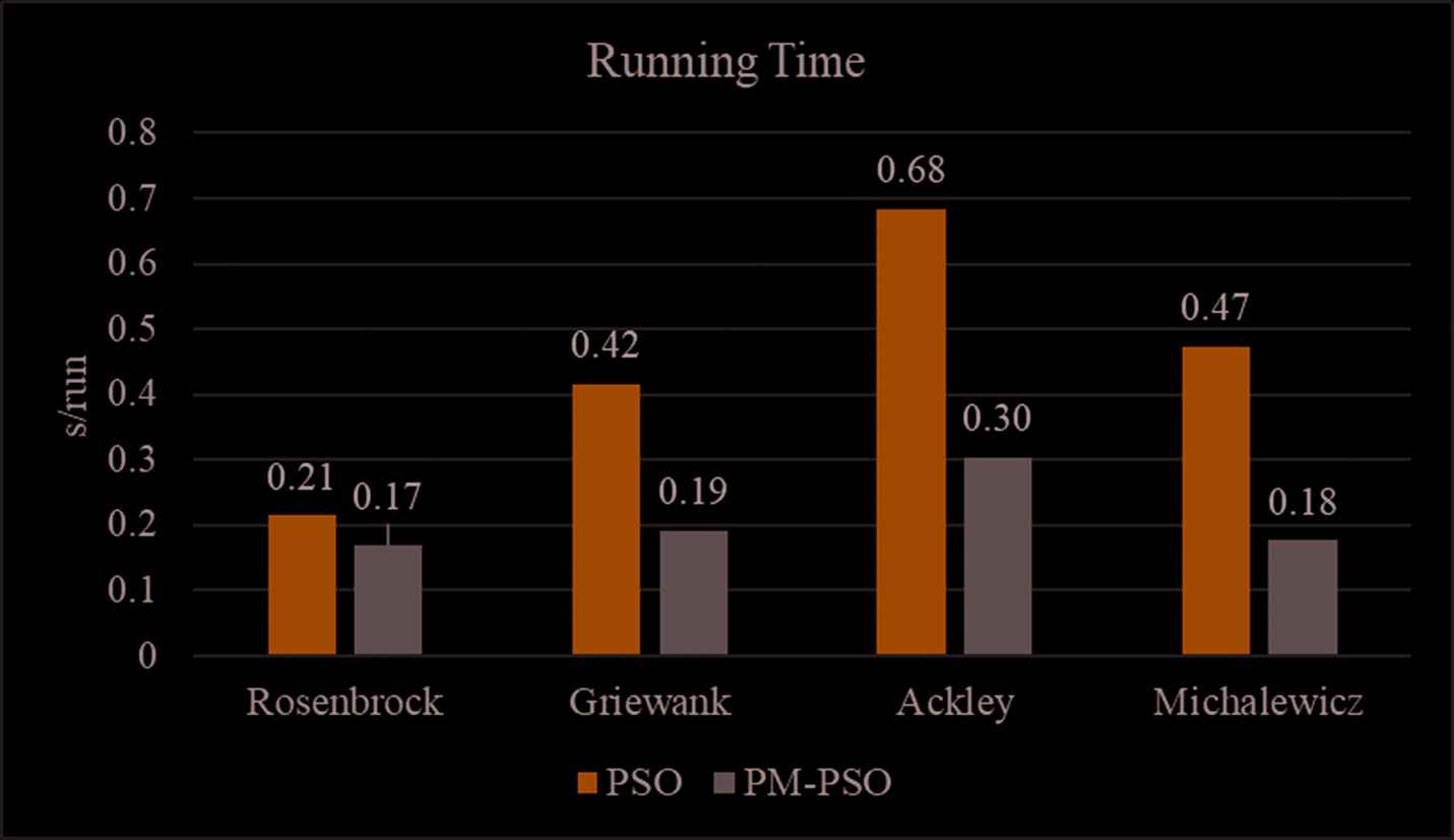
Running time of standard particle swarm optimization (PSO) compared to proposed PM-PSO.
In the case of the optimization of the Griewank using PM-PSO, the searching region [−600; 600] is divided into four sub-regions [[−600; −300]; [−300; 0]; [0; 300]; [300; 600]] according to
5.2. Proposed PM-PSO Method Applied in Optimization of FOC-PID Parameters
For each case, 10 independent classical PSO training tests are investigated and the statistical results related to the J value, training time are completely shown in Tables 4–7.
| Number of Calculation Loop | SPSO | Proposed PM-PSO | ||
|---|---|---|---|---|
| Total Generation | PopSize | Total Generation | PopSize | |
| 200 | 10 | 24 | 10 | 6 × 4 |
| Runtime | J value | Training time (sec) | J value | Training time (sec) |
| 1 | 6.2170e+03 | 982.6 | 5.7058e+03 | 349.5 |
| 2 | 6.3356e+03 | 988.6 | 4.9523e+03(*) | 313.2 |
| 3 | 5.7399e+03 | 995.3 | 6.4139e+03 | 303.5 |
| 4 | 5.2306e+03 | 986.3 | 5.1691e+03 | 300.9 |
| 5 | 5.3676e+03 | 970.5 | 6.5410e+03 | 299.9 |
| 6 | 6.0665e+03 | 967.5(*) | 5.7916e+03 | 298.7(*) |
| 7 | 5.2380e+03 | 984.4 | 7.1795e+03 | 304.3 |
| 8 | 4.7115e+03 | 972.0 | 5.3953e+03 | 303.1 |
| 9 | 4.4546e+03(*) | 981.8 | 5.0330e+03 | 304.6 |
| 10 | 5.0771e+03 | 970.3 | 5.7747e+03 | 309.1 |
| Mean | 5.4400e+03 | 979.9 | 5.8000e+03 | 308.7 |
SPSO, standard particle swarm optimization; PSO, particle swarm optimization
Case 1 – 10gen24particle.
| Number of Calculation Loop | SPSO | Proposed PM-PSO | ||
|---|---|---|---|---|
| Total Generation | PopSize | Total Generation | PopSize | |
| 300 | 10 | 48 | 10 | 12 × 4 |
| Runtime | J value | Training time (sec) | J value | Training time (sec) |
| 1 | 5.1414e+03 | 1969.6 | 4.9245e+03 | 604.3 |
| 2 | 5.3568e+03 | 2051.3 | 4.6878e+03 | 600.2 |
| 3 | 4.7614e+03 | 2081.1 | 5.1898e+03 | 601.0 |
| 4 | 5.1346e+03 | 1974.0 | 4.5614e+03 | 604.4 |
| 5 | 4.6158e+03 | 1966.9 | 4.4830e+03 | 603.8 |
| 6 | 5.8932e+03 | 1965.5 | 4.4384e+03(*) | 597.7(*) |
| 7 | 4.4208e+03(*) | 1966.5 | 6.5609e+03 | 603.2 |
| 8 | 4.4246e+03 | 1999.8 | 5.6027e+03 | 601.2 |
| 9 | 6.6357e+03 | 1971.0 | 5.2908e+03 | 601.1 |
| 10 | 4.6925e+03 | 1962.4(*) | 5.1543e+03 | 599.8 |
| Mean | 5.1100e+03 | 1990.8 | 5.0900e+03 | 601.7 |
SPSO, standard particle swarm optimization; PSO, particle swarm optimization
Case 2 – 10gen48particle.
| Number of Calculation Loop | SPSO | Proposed PM-PSO | ||
|---|---|---|---|---|
| Total Generation | PopSize | Total Generation | PopSize | |
| 400 | 10 | 60 | 10 | 15 × 4 |
| Runtime | J value | Training time (sec) | J value | Training time (sec) |
| 1 | 5.4947e+03 | 2440.3 | 4.4346e+03 | 752.3 |
| 2 | 4.4797e+03 | 2455.1 | 4.4370e+03(*) | 750.9 |
| 3 | 4.4787e+03 | 2820.5 | 5.3184e+03 | 743.7(*) |
| 4 | 4.4246e+03(*) | 2496.6 | 4.5327e+03 | 748.1 |
| 5 | 6.2065e+03 | 2435.6 | 5.1911e+03 | 753.1 |
| 6 | 6.0658e+03 | 2435.6 | 5.6657e+03 | 770.5 |
| 7 | 5.8426e+03 | 2321.4 | 4.8502e+03 | 779.0 |
| 8 | 4.4703e+03 | 2302.9 | 4.4719e+03 | 778.0 |
| 9 | 4.4347e+03 | 2291.5(*) | 5.3862e+03 | 764.5 |
| 10 | 4.4544e+03 | 2297.4 | 4.5680e+03 | 756.0 |
| Mean | 5.0400e+03 | 2429.8 | 4.8900e+03 | 759.6 |
SPSO, standard particle swarm optimization; PSO, particle swarm optimization
Case 3 – 10gen60particle.
| Number of Calculation Loop | SPSO | Proposed PM-PSO | ||
|---|---|---|---|---|
| Total Generation | PopSize | Total Generation | PopSize | |
| 400 | 10 | 72 | 10 | 18 × 4 |
| Runtime | J value | Training time (sec) | J value | Training time (sec) |
| 1 | 4.8721e+03 | 2767.6 | 4.9562e+03 | 898.3 |
| 2 | 4.5403e+03 | 2751.7 | 4.6085e+03 | 893.9 |
| 3 | 5.1795e+03 | 2774.0 | 5.5953e+03 | 890.1 |
| 4 | 6.0641e+03 | 2775.9 | 4.7629e+03 | 887.6 |
| 5 | 4.5016e+03 | 2765.3 | 5.1834e+03 | 888.0 |
| 6 | 4.4239e+03 | 2765.8 | 4.7745e+03 | 889.7 |
| 7 | 4.9346e+03 | 2765.6 | 5.0763e+03 | 889.2 |
| 8 | 4.4156e+03(*) | 2751.2(*) | 4.6017e+03(*) | 884.6(*) |
| 9 | 4.4768e+03 | 2756.5 | 5.0967e+03 | 888.7 |
| 10 | 4.4788e+03 | 2764.3 | 5.0502e+03 | 892.1 |
| Mean | 4.7900e+03 | 2763.79 | 4.9700e+03 | 890.2 |
Bold(*) is the best result of each case in SPSO and PM-PSO experiment.
Bold(**) is the best result of J value and training-time in each method.
SPSO, standard particle swarm optimization; PSO, particle swarm optimization
Case 4 – 10gen72particle.
The best results of four testing cases shown in Tables 4–7 are concisely tabulated in Table 8 as follows,
| SPSO | PM-PSO | Ratio |
|||
|---|---|---|---|---|---|
| Case | J | Training Time (sec) | J | Training Time (sec) | |
| 1 | 5.4400e+03 | 979.9 | 5.8000e+03 | 308.7 | 3.174 |
| 2 | 5.1100e+03 | 1990.8 | 5.0900e+03 | 601.7 | 3.309 |
| 3 | 5.0400e+03 | 2429.8 | 4.8900e+03 | 759.6 | 3.199 |
| 4 | 4.7900e+03 | 2763.8 | 4.9700e+03 | 890.2 | 3.105 |
SPSO, standard particle swarm optimization; PSO, particle swarm optimization
Best results of four testing cases.
Table 8 shows that the training time of SPSO implemented on single core takes 979.9s in total by 10 generations and 24 particles meanwhile it takes 1990.8s by 10 generations and 48 particles. It also takes 2429.8s in total by 10 generations and 60 particles. Eventually in the last case it takes 2763.79s by 10 generations and 72 particles. We see that the fitness value decrease significantly when the experiment carried out more number of generations and particles. As presented in Table 8, the proposed PM-PSO method not only generate outperforming results compared to SPSO but also found more fitting solution for optimizing PID parameter due to J value quickly converging to minimum. The experiment results show that PM-PSO providing more precise and stable outcome than SPSO.
In Table 8, the training time of PM-PSO, implemented on 4 cores, is excellently ameliorated and reduced to only 308.7s in case of 10 generations and 6 particles meanwhile it takes 601.7s in case of 10 generations and 12 particles, 759.6s in total in case of 10 generations and 15 particles and eventually the case of 10 generations and 18 particles it takes 890.2s. Using the last “ratio” column of Table 8, which is clear to note that the training time of the optimized PID parameters using SPSO technique on single core are quite worse than the training time of proposed PM-PSO executing on multi-core over 310%.
The results are shown in Tables 4–7. Those experiments show that the mean value of J value reduces gradually when the number of particle increased from 24 to 72 particles. It means the proposed algorithm returned the stable results from independence cases when the number of particles is increasing.
In detail, the resulted optimized PID parameters of three PI blocks, implemented in BLDC FOC-PID controller, using PM-PSO and SPSO are adequately shown in Tables 9 and 10, respectively.
| Case | Generation | PopSize | P1 | P2 | P3 | I1 | I2 | I3 |
|---|---|---|---|---|---|---|---|---|
| 1 | 10 | 24 | 20 | 1.2460 | 1 | 0.9283 | 0 | 0 |
| 2 | 10 | 48 | 0.4108 | 0.6623 | 1 | 10 | 0 | 0 |
| 3 | 10 | 60 | 0 | 1.2771 | 1 | 10 | 0 | 0 |
| 4 | 10 | 72 | 0.5117 | 0.6619 | 1 | 0.4515 | 0 | 0 |
PID, proportional integral derivative; SPSO, standard particle swarm optimization.
Resulted optimized PID parameters of SPSO.
| Case | Generation | PopSize (×4) | P1 | P2 | P3 | I1 | I2 | I3 |
|---|---|---|---|---|---|---|---|---|
| 1 | 10 | 6 | 0.1362 | 1.4686 | 0.4238 | 8.3042 | 4.5211 | 0 |
| 2 | 10 | 12 | 0 | 1.2857 | 1 | 0 | 0 | 0 |
| 3 | 10 | 15 | 0 | 1.2801 | 1 | 0 | 0 | 0 |
| 4 | 10 | 18 | 0 | 1.2824 | 1 | 0.6217 | 0 | 0.6816 |
PID, proportional integral derivative; SPSO, standard particle swarm optimization.
Resulted optimized PID parameter of PM-PSO
Figure 9 shows the step response of the proposed PMPSO-PID and standard PSO-PID FOC BLDC controller for all cases in which the eventual resulted optimized PID parameter using proposed PMPSO and standard PSO shown in Table 11. The best response for each test-case is shown in Figure 9 where the recovery time reaches the reference mechanical angle of BLDC motor around 0.09s. The overshoot of step response is decreased significantly when the number of both generation and particle is increased. Figure 9 shows the step response of the closed loop BLDC system by using proposed parallel PMPSO algorithm that the recovery time reaches the reference mechanical angle of BLDC motor around 0.2s as same rate as one using SPSO algorithm.

Comparative step responses of proposed parallel multi-population particle swarm optimization (PMPSO)-proportional integral derivative (PID) and standard particle swarm optimization (SPSO)-PID field-oriented control (FOC) brushless DC electric motor (BLDC) controller.
| PM-PSO PID | Standard SPSO PID | ||
|---|---|---|---|
| PI angular velocity | P3 | 1 | 1 |
| I3 | 0 | 0 | |
| PI iq | P2 | 1.2801 | 1.2771 |
| I2 | 0 | 0 | |
| PI id | P1 | 0 | 0 |
| I1 | 0 | 10 | |
| Max overshoot | % | 23.74 | 23.85 |
| Steady state theta value | theta | 1.049 | 1.053 |
| Steady state error | e (%) | 0.19 | 0.57 |
PID, proportional integral derivative; SPSO, standard particle swarm optimization.
Eventual resulted optimized PID parameters.
Figure 9 and Table 11 comparatively show the best case of performance responses of closed loop BLDC system between proposed Parallel multi PM-PSO and standard SPSO algorithm. Those results confirm that the proposed parallel multi PM-PSO proves better than standard SPSO algorithm not only in steady-state error but also in transient-time response.
Eventually the comparative convergence curve of proposed parallel multi PM-PSO and standard SPSO algorithm are shown in Figure 10. Those results demonstrate that the proposed parallel multi PM-PSO obtains better fitness value than standard PSO algorithm not only in optimally minimum fitness value but also in number of converging iterations.
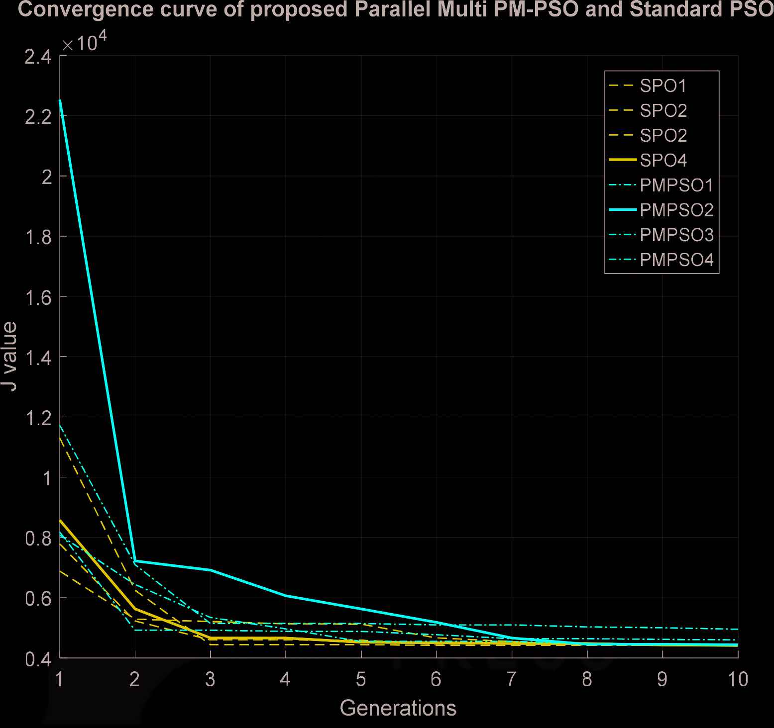
Convergence curve of proposed parallel multi PM-particle swarm optimization (PSO) and standard PSO.
6. CONCLUSIONS
In this work, a comparison of using proposed PMPSO-PID and standard SPSO-PID for optimally identifying PID parameters of BLDC FOC-PID controller is satisfactorily shown. Moreover, the well-known benchmark functions such as Rosenbrock, Griewank, Ackley, and Michalewicz are used to test proposed technique. The results show that multi-population technique applied on PM-PSO algorithm achieves competitive performance compared to the standard SPSO one. The results show that the proposed PMPSO-PID controller performs an efficient tuning method for PID parameters. By comparing between proposed PMPSO-PID and standard SPSO-PID, it shows that both of PM-PSO and SPSO algorithm enhance the dynamic performance of the closed loop BLDC system. As a consequent the parallel multi-population (PM) technique applied on PM-PSO optimization algorithm which yields superior results compared to the classical ones in running-time requirement.
CONFLICTS OF INTEREST
The authors have declared that there is no conflicts of interest.
AUTHORS' CONTRIBUTIONS
Nguyen T.D.: original idea, edit the draft, prepare software and source code. Cao V.K.: improve idea, complete source code. Ho P.H.A.: complete the content and edit the final paper.
ACKNOWLEDGMENTS
We acknowledge the support of time and facilities from Ho Chi Minh City University of Technology (HCMUT), VNU-HCM for this study.
REFERENCES
Cite this article
TY  - JOUR
AU  - Nguyen Tien Dat
AU  - Cao Van Kien
AU  - Ho Pham Huy Anh
PY  - 2021
DA  - 2021/03/25
TI  - Optimal FOC-PID Parameters of BLDC Motor System Control Using Parallel PM-PSO Optimization Technique
JO  - International Journal of Computational Intelligence Systems
SP  - 1142
EP  - 1154
VL  - 14
IS  - 1
SN  - 1875-6883
UR  - https://doi.org/10.2991/ijcis.d.210319.001
DO  - 10.2991/ijcis.d.210319.001
ID  - Dat2021
ER  -