
Dynamic Relationship Network Analysis Based on Louvain Algorithm for Large-Scale Group Decision Making
 , Tao Jiang1, Witold Pedrycz2, 3
- DOI
- 10.2991/ijcis.d.210329.001How to use a DOI?
- Keywords
- large-scale group decision making; consensus reaching process; dynamic relationship network; Louvain algorithm; node centrality; subgroup cohesion
- Abstract
In most existing large-scale group decision making (LSGDM) problems, the relationships between decision makers (DMs) are usually ignored or regarded as static. However, in many cases, the results of LSGDM are dynamically influenced by the relationship between group members. To address this issue, a dynamic relationship network analysis method based on Louvain algorithm is proposed in this paper. First, each DM could be considered as a node to construct a relationship network, which dynamically change the individual opinion by the definition of correction index to eliminate subjective factors. Second, the node centrality and subgroup cohesion are defined and the Louvain algorithm is used to divide DMs into several subgroups to measure the importance of each node and subgroup. Then, the termination conditions of the discussion are determined by measuring the consensus and stability of the group decision information. Moreover, stage weight function is defined to assign weights to discussions at different stages and obtain the final results. An illustrative example is provided to prove the feasibility of the proposed model. Sensitivity analysis is given to show the stability of correction index and stage weight function. Finally, the comparative analysis is performed to illustrate its feasibility and effectiveness of the method.
- Copyright
- © 2021 The Authors. Published by Atlantis Press B.V.
- Open Access
- This is an open access article distributed under the CC BY-NC 4.0 license (http://creativecommons.org/licenses/by-nc/4.0/).
1. INTRODUCTION
Nowadays, due to the rapid development of social network analysis (SNA), large-scale group decision making (LSGDM) problems with social relationship has become a hot topic in decision analysis area [1]. Definitely, LSGDM can be regarded as a process where a large group of decision makers (DMs) try to reach consensus to a problem consisting of multiple possible solutions [2]. However, the rapid information dissemination speed and many factors in consensus reaching process (CRP) have made a successful group decision making (GDM) more and more difficult [3]. In addition, with the increasing public awareness of democratic participation, the timeliness of news and the rapid access to information, more and more people are willing to participate in the LSGDM activities. These phenomena have led to the traditional LSGDM model urgently needs to consider the real life situation and practical significance [4].
LSGDM based on SNA has been a quite popular research topic during the last decade [5–13]. Recently, Wu et al. [14] proposed a two-stage solution based on trust networks information modeling, which not only reduce the complexity for LSGDM problems, but also improve the reliability of the decision results as well. Moreover, Gai et al. [15] proposed a joint feedback strategy based on harmony degree to help the multiple non-consensus decision makers modify their preferences to improve the efficiency of consensus achievement. To deal with the vague and uncertain features in complex micro-grid planning problems, Ren et al. [16] used hesitant fuzzy linguistic term sets (HFLTSs) to express experts’ opinions, and introduced a novel SNA-based clustering method to classify them. Besides, this model also considered the minority opinions in a micro-grid planning problem and provided an approach to manage these opinions. In order to explore the evolution of consensus, Wu et al. [17] proposed a new CRP tool based on consensus evolution networks (CENs). With the help of the CENs, the consensus measure and feedback adjustment in CRP are processed with an important advantage, managing the consensus thresholds and its evolution process.
Because of the number of DMs in LSGDM problems is often more than 20, usually, it is necessary to divide them into several groups according to certain relationships, and thus, the clustering algorithm is one of the most key factors in the development of CRP. However, there are two different ways to improve clustering algorithms in LSGDM problems. On the one hand, some studies mainly focus on the optimization technique of traditional clustering algorithms for dealing with LSGDM problem [18,19]. For example, Waltman and Eck [20] developed a new algorithm for community detection based on modularization in large network. This algorithm used a local mobile heuristic in a more complex way, and its computational efficiency can perform community detection in a network with tens of millions of nodes and hundreds of millions of edges in a short calculation time. Furthermore, Ding et al. [21] proposed a sparse representation-based intuitionistic fuzzy clustering (SRIFC) algorithm to solve LSGDM problems. According to the demonstrative experimental results, the proposed algorithm is adaptive and unsupervised to detect the communities. Meanwhile, Chu et al. [22] proposed a social network community detection method based on the fuzzy clustering and a repairing incomplete fuzzy preference relations method based on the divided communities. Based on this, they proposed a two-stage CRP method to balance the number of discussions and modification range of original decision information.
In summary, despite the extensive prior research proposed SNA models and optimization clustering algorithms in LSGDM problems. They still suffer from some limitations. For example, the existing studies seldom consider the dynamic network relationship, they often only use the static network to solve LSGDM problems. Considering the dynamic relationship network between DMs will affect the CRP and meet the needs of modern society, it will inevitably become one of the key research directions in LSGDM [23]. The challenges in LSGDM research mainly focus on the following three aspects [24,25]:
Only a small number of studies consider how to identify the status of each DM and modify the GDM information to achieve more objective and reasonable results because of the large differences among DMs.
Traditional clustering algorithms which only focus on the opinion or preference matrix of DMs are not realistically applicable for the LSGDM problems where there are strong social relationships between DMs.
In the existing SNA-based models, the relationship propagation operators do not consider how to effectively coordinate different preferences of DMs in a short period of time when individual opinions are scattered.
In order to overcome the research gaps of the current studies, this paper will propose a novel dynamic relationship network based on Louvain algorithm [26] for solving LSGDM problems. And since the CRP is used to simulate the actual situation, it is necessary to consider the impact of real situation. In this paper, we assume that the opinion of DM will be affected by the order of alternatives through the evaluation process, which is a common behavior in reality. For example, in a talent show, if the performance level of the actors is roughly the same, the scores of the first few actors are often higher. On the contrary, the scores of the last few actors will be lower, while the scores of the middle actors will be more objective. Based on this social phenomenon, we define the correction index and simulate it, then a sensitivity analysis is given to show its stability. And regarding to evolution of LSGDM consensus network, we introduce the Louvain algorithm instead of fuzzy c-means (FCM), and the comparative analysis is provided to prove its dynamicity and feasibility. Finally, an illustrative example is provided to verify the scientific nature of consensus process and the practicality of optimization model.
The motivation of this study is to reach consensus with dynamic SNA method and simulate real social phenomenon with the mathematical model. In that case, we develop this model not only scientific in mathematical sense, but also in practical problems.
The main contributions of this study are summarized as follows:
Define a new correction index. Correction index is defined to reasonably simulate the social phenomenon that the order of alternatives will affect the opinion of DM. In other words, it is used to make reasonable corrections in order to reduce or eliminate the subjective influence of DMs.
Provide a dynamic relationship network in CRP. A new dynamic relationship network is used to reflect the relationship between DMs in the LSGDM problems. According to the definition of GDM model and node importance evaluation, the DM’s opinion on the alternatives will be adaptively adjusted as the social network changes, while the social network will also be adaptively adjusted with the DM’s opinion, which eventually obtains a dynamic CRP network.
Community detection driven by using Louvain algorithm. The Louvain algorithm [26] is used to solve the network clustering problems in this study. Compared with FCM algorithm, Louvain algorithm is simple, fast, accurate and efficient. According to the definition and properties of modularity, it has more advantages than other clustering algorithms in dealing with dynamic social network problems.
The rest of this paper is organized as follows: Section 2 introduces the preliminaries about LSGDM problems. Section 3 constructs the dynamic relationship network to offset personal subjective impact with a certain correction index. Section 4 proposes the LSGDM model based on dynamic relationship network analysis. Section 5 provides an illustrative example to illustrate the feasibility of proposed model. The conclusions are given in Section 6.
2. PRELIMINARIES
2.1. Score Matrix in GDM
Suppose that there are
2.2. Large-scale Group Decision Making
The concept of LSGDM has been studied more widely than GDM because of the social demand for group participation in important decision process [27]. Although the basic concepts of them are quite similar, there is a big difference is that the number of DMs. The number of DMs in LSGDM is much greater than that in GDM. In general, a LSGDM problem consists of an alternative set
2.3. Consensus Reaching Process
To eliminate the conflict among DMs by reducing it under an acceptable degree for GDM, a comprehensive used approach consists in undertaking a CRP, aimed at obtaining a collective solution as close as possible to unanimous agreement [11]. It involves the following steps [29,30].
Step 1. Initial decision. The DM
Step 2. Interactive decision. The DM
Step 3. Termination of discussion. When the termination condition of the discussion is reached, the discussion stops. Then the stage weight
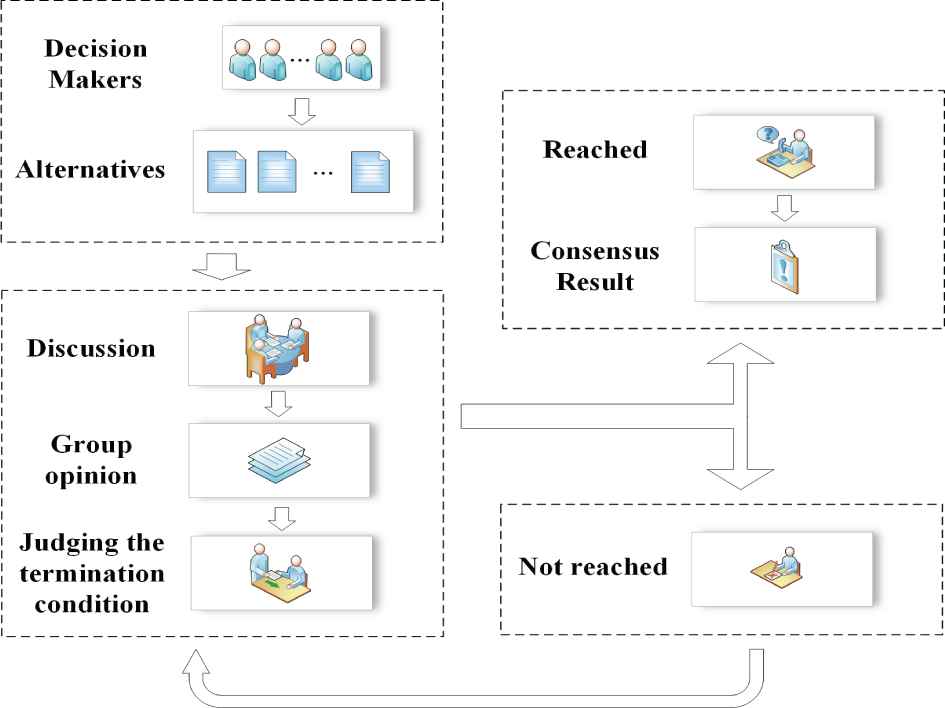
The framework of CRP.
3. CONSTRUCTION OF DYNAMIC RELATIONSHIP NETWORK
3.1. Definition of Correction Index
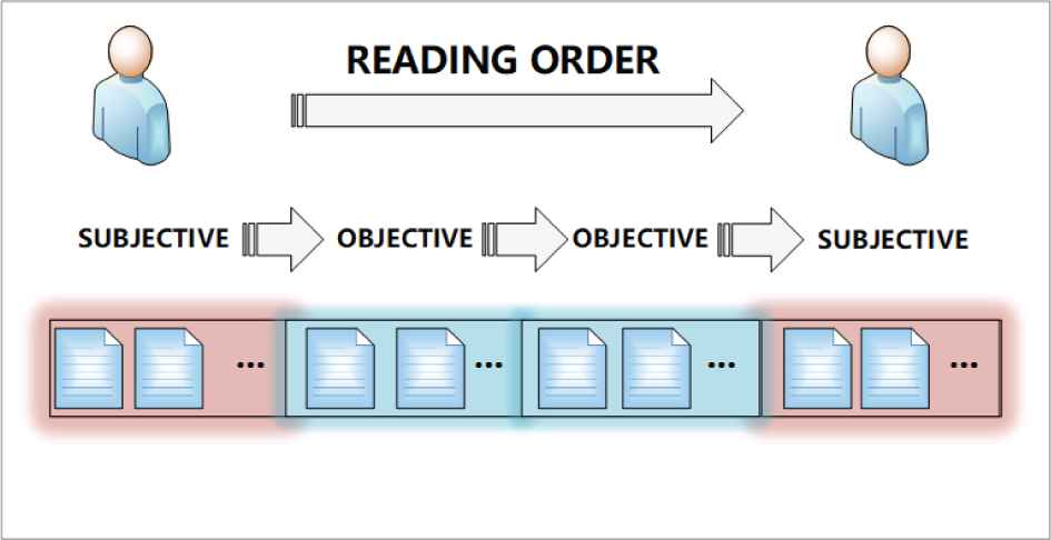
Due to the subjective factors on DMs in the process of scoring, and the order of alternatives will cause the decision-making score to deviate from objective facts, so it is necessary to offset personal subjective impact with a certain correction index when the DM scores. The DM’s emotional change process is shown in Figure 2.
Scoring process.
Firstly, we set three parameters
The definition of correction index
Definition 1.
In the
In Eq. (4),
The score after correction is defined as:
In Eq. (5),
Then the correction vector and matrix are defined as:
Definition 2.
The correction vector corresponding to the score vector
And the correction matrix of the
3.2. Dynamic Relationship Network
The relationship network includes the following key concepts: nodes, relationship connections, subgroups, and relationship network analysis. Nodes represent DMs, which are connected through some types of relationship to form a network structure. Subgroups represent any subset of nodes in the network and all connections between them.
Definition 3.
[31] In the
For such a complex LSGDM problems, decision-making information enables DMs to be related to each other instead of isolated individuals, which is the key issue to establishing a relationship network structure. Regarding to the score of each stage
Based on the above analysis, the correlation coefficient value is now converted into binary data of
Construct a relationship network graph and a symmetric relation matrix of
4. DECISION-MAKING METHOD BASED ON DYNAMIC RELATIONSHIP NETWORK ANALYSIS
4.1. Node Importance Evaluation
In relationship networks, the importance of each node is not exactly the same. Based on the establishment of the relationship network structure, this study uses the measurement of node centrality to determine the weight, and then normalizes the node centrality to obtain the node importance. Node centrality reflects the connection relationship between each node and other nodes in the relationship network. A node with a high degree of value has a direct or adjacent relationship with other nodes, which also indicates that the node occupies the center position of the network, and the nodes with low degrees of value are obviously in the periphery of the network. If a node is completely isolated, removing it will have no effect on the whole network.
In other words, the node centrality is a measure of the consensus between the individual opinion and the group opinion in LSGDM. And the evaluation of node importance is based on the DM’s scoring information, so it will make the decision-making results more reasonable and objective.
Definition 4.
[20] In the
And the weight of node
Definition 5.
The weight of node
4.2. Group Decision Making Model
In the
The normalized weight corresponding to node
Definition 6.
Let
And
Combining all of the above parameters, the standardized decision-making results for each stage is obtained.
Definition 7.
The single-stage decision-making results
In this equation,
Then the total decision results
The essence of the model is the horizontal aggregation of the decision-making information of the single-stage solution, and the results of the single-stage solution are assembled vertically by the stage weights to obtain the final ranking.
4.3. Louvain Algorithm and Subgroup Weight Analysis
4.3.1. Louvain algorithm
The Louvain algorithm is a new community detection algorithm based on modularity [32]. This algorithm performs well in efficiency and effectiveness, and can discover hierarchical community structures. Its optimization goal is to maximize the modularity of the entire community network.
Modularity is an important measure to evaluate the quality of a community network. Its physical meaning is the difference between the number of node’s sides in the community and the number of edges in a random case, and its value range is [−0.5, 1], and the equation is shown as [33]:
In this equation,
Definition 8.
[33] Suppose that there is
The Louvain algorithm involves the following steps.
Step 1. Let each node in the graph as an independent community with the same number of communities as the number of nodes.
Step 2. For each node
Step 3. Repeat Step 2 until the community of all nodes no longer change.
Step 4. Compress all nodes in the same community into a new node. The weight of edges between nodes in the community is transformed into the weight of the new node, and the edge weights between communities are transformed into edge weights between new nodes.
Step 5. Repeat Step 1 until the modularity of the entire graph no longer change.
According to the above steps, the Louvain algorithm is summarized in Algorithm 1 as follows.
Algorithm 1 Louvain algorithm
1: Let each node
2: while all nodes no longer change
3: Assign node
4: Calculate the change of modularity
5: if
6: Assign node
7: else
8: Continue;
9: end if
10: Compress all nodes in the same community;
11: Calculate new weight of edges;
This change of scales, that is, from around 5 million nodes for other clustering algorithms to more than 100 million nodes in this algorithm, opens exciting perspectives as the modular structure of complex systems such as whole countries or huge parts of the Internet can now be unraveled. The accuracy of this algorithm has also been tested on ad hoc modular networks and is shown to be excellent in comparison with other (much slower) community detection algorithms [26].
4.3.2. Subgroup weight analysis
Subgroup is a subset of nodes that have stable and frequent connections with each other. It is a simplification of the complex and huge overall network structure. Since the accuracy of the aggregated decision information of the entire group is required, not only the internal members of the subgroup are closely connected, but also the subgroup and the external members must have close communication. The degree of cohesion of a subgroup is derived from the relative strength or density of the internal connections of the subgroup, and the relative strength, sparseness, or density of the connections between members of the subgroup and non-members.
In other words, the degree of subgroup cohesion is not only reflected in the sum of the strength of the internal and external connections of the subgroup, but also intuitively shows the internal relationship between the subgroup and the overall network structure. Therefore, the degree of subgroup cohesion is the most direct way to determine the weight of the subgroup.
The definition of agglomeration degree and weight of subgroup
Definition 9.
In the
In virtue of Eq. (18),
And the subgroup weight
4.3.3. Termination condition
In LSGDM problems, the purpose of discussion is to allow members to continuously modify their evaluation information through information discussion and eventually the GDM information reaches a relatively stable and consistent state. Therefore, the consensus and stability of GDM information need to be objectively measured in the entire process to determine the termination conditions of the discussion.
Network graph density is a measure of the connections between nodes in the entire relationship network. The higher the network graph density is, the more connections between nodes. Because of the relationship network which is developed based on the consensus of information among groups, the greater the density of the network graph, the larger amount of relatively consistent information among DMs, and the more consistent the group’s opinions within the stage. It means that the density of network graphs can be used as a measure for the consensus of GDM information in the stage.
The definition of group consensus index in the
Definition 10.
In the
Where
The stability index of the
Definition 11.
Let
In this equation,
During the
4.3.4. Determination of discussion weights
The discussion weight function mainly describes the importance of the evaluation data information at the
Based on the above analysis of stage weights and their requirements, we find
Stage weight function.
The definition of stage weight
Definition 12.
Let
In this equation,
In summary, according to the above principles and methods to obtain the DM’s weight
4.4. The Proposed CRP Framework Based on Dynamic Relationship Network
In this section, we combine all of the previous approaches together and propose a completely new CRP framework based on dynamic relationship network [35,36]. A new set of rules has been developed for the entire CRP, as shown in Figure 4.
Consensus improvement process.
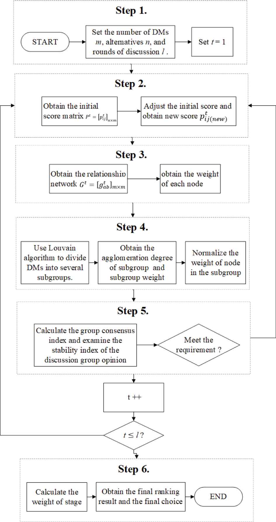
Step 1. Collect the score information of all
Step 2. The correction index
Step 3. Collect the relationship network
Step 4. The Louvain algorithm is used to divide DMs into several subgroups to measure the importance of each node and subgroup. And the agglomeration degree of subgroup
Step 5. Using Eq. (20) to calculate the group consensus index and Eq. (21) to examine the stability index of the discussion group opinion. If both of them are meet the requirement, then we obtain the single-stage ranking result by Eq. (14), otherwise we have the next round of discussion.
Step 6. When all rounds of discussion finish, we use Eq. (22) to calculate the weight of stage which meet the requirement. Then we obtain the final ranking result and the optimal choice.
5. ILLUSTRATIVE EXAMPLE
5.1. Problem Description
Suppose that there is a decision-making group with 20 DMs
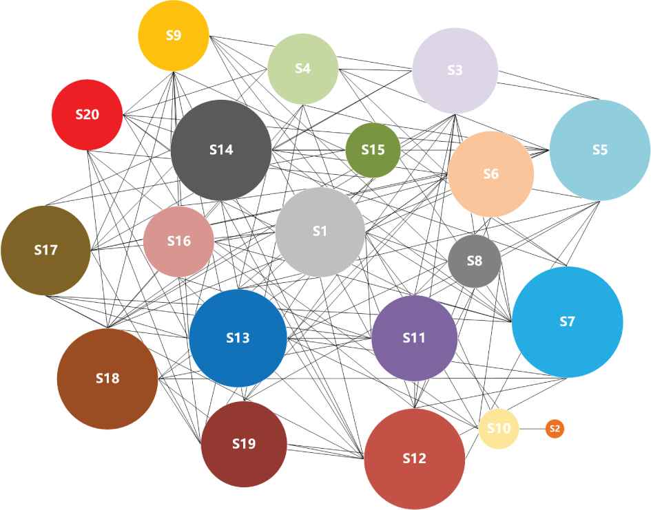
Relationship network topology diagram.
Taking the first round of discussion as an example. We obtain the score matrix
In Eq. (3), we set the correction threshold
According to Eq. (5), the new score matrix
In virtue of Eq. (9), the relationship matrix and its topology diagram are obtained as follows:
Finally, the new score matrix
Similarly, we can obtain the new score matrix
| Stage | ||||||||||
|---|---|---|---|---|---|---|---|---|---|---|
| 0.056 | 0.004 | 0.052 | 0.049 | 0.065 | 0.052 | 0.068 | 0.032 | 0.049 | 0.024 | |
| 0.044 | 0.052 | 0.048 | 0.056 | 0.068 | 0.039 | 0.044 | 0.016 | 0.056 | 0.044 | |
| 0.054 | 0.054 | 0.050 | 0.050 | 0.064 | 0.046 | 0.043 | 0.028 | 0.064 | 0.039 | |
| 0.046 | 0.059 | 0.053 | 0.049 | 0.063 | 0.049 | 0.046 | 0.033 | 0.059 | 0.036 | |
| Stage | ||||||||||
| 0.052 | 0.035 | 0.060 | 0.065 | 0.036 | 0.049 | 0.056 | 0.065 | 0.052 | 0.049 | |
| 0.059 | 0.056 | 0.044 | 0.068 | 0.035 | 0.044 | 0.056 | 0.064 | 0.059 | 0.048 | |
| 0.068 | 0.050 | 0.043 | 0.046 | 0.050 | 0.043 | 0.054 | 0.061 | 0.057 | 0.036 | |
| 0.063 | 0.053 | 0.039 | 0.053 | 0.059 | 0.043 | 0.046 | 0.059 | 0.053 | 0.039 |
Weights of DMs.
Based on Louvain algorithm, the DMs set
| Stage | ||||
|---|---|---|---|---|
| Stage | ||||
| – | ||||
| – | – | – |
Subgroup clustering results.
| Stage | |||||||
|---|---|---|---|---|---|---|---|
| t = 1 | 0.109 | 0.105 | 0.246 | 0.165 | 0.105 | 0.056 | 0.214 |
| t = 2 | 0.230 | 0.238 | 0.250 | 0.056 | 0.101 | 0.125 | 0 |
| t = 3 | 0.214 | 0.221 | 0.113 | 0.073 | 0.052 | 0.117 | 0.210 |
| t = 4 | 0.383 | 0.169 | 0.206 | 0.242 | 0 | 0 | 0 |
Subgroup weight.
Using Eqs. (14) and (15), the evaluation information
Similarly, based on Eqs. (20) and (21), the consensus and stability indicators of group opinions are calculated as follows:
According to Eq. (22), the stage weight is determined
Linearly weight alternative by stage weights, the results are:
The ranking results of alternatives
5.2. Sensitivity Analysis
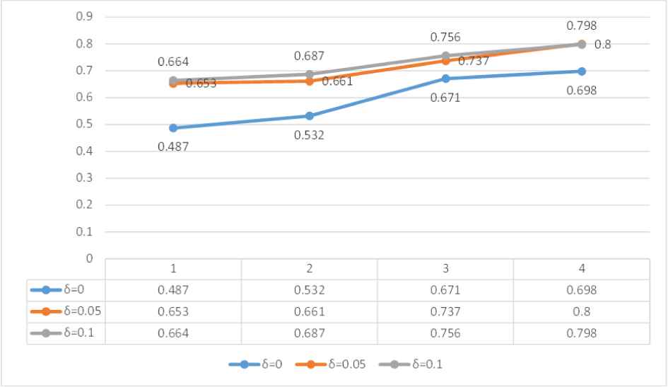
5.2.1. Impact of δ
In order to test the stability of the proposed model, we carry out sensitivity analysis of the subgroup by changing the correction rate
| Weight Vector | Ranking Results | |
|---|---|---|
| 0.05 | ||
| 0.10 | ||
| 0.15 | ||
| 0.20 | ||
| 0.25 | ||
| 0.30 |
Ranking results.
As the value of
It is worth mentioning that when
In Figure 6, we can see that the group consensus of our proposed model is greater than that of the general model in each round of stage. Moreover, the consensus in some stages in the general model is even lower than the lower limit set in this study. We can assume that it is due to the correction of the initial score matrix by our CRP model, which makes it easier for them to achieve a high degree of consensus without affecting the score matrix.
Group consensus result.
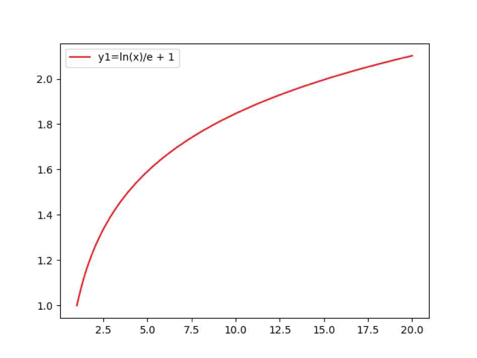
5.2.2. Impact of stage weight function f ( x )
If there is only one round of discussion, then the weight of this round of discussion is 1, so there is
In general,
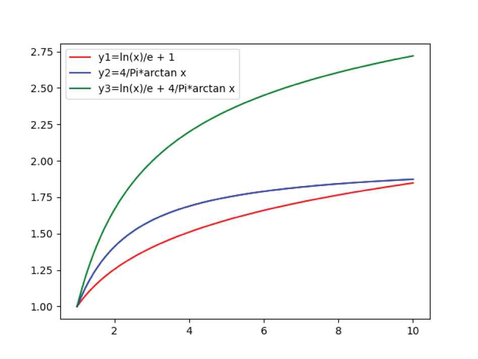
In addition to the functions used in this study, we have defined three functions for further analysis, which are shown as follows:
The images of the three functions are shown in Figure 7, the x-axis indicates the number of discussions, and the y-axis indicates the function value.
Three optional stage weight function.
When the number of discussions is small, the previous discussions have reference value, so its weight will not be much smaller than that of the later discussions. While the number of discussions is too large, the reference value of the first few times can be almost ignored. At this time, the weight of the next few times is much more important than the previous few times. In Figure 7, we can see that
Moreover, although both
5.2.3. Comparative analysis
To illustrate the validity of the proposed model, we compare the proposed model with consensus model for LSGDM considering non-cooperative behaviors and minority opinions in [23]. The model in [23] is applied to the case in this study and the results are shown in Table 5. Among them,
| Ranking Results | |||||
|---|---|---|---|---|---|
| 0.319 | 0.804 | ||||
| 0.237 | 0.761 | 0.776 | |||
| 0.262 | 0.770 | ||||
| 0.182 | 0.755 |
Obtained results in [23].
It is apparent that from Table 5, the optimal alternative of both models is
| Evaluation Measures | The Proposed Model in this Study | The Model in [23] |
|---|---|---|
| Clustering results | The Louvain algorithm is used to adaptively adjust subgroups from the initial 7 to 4 after 4 rounds of clustering. | Specify the number of clusters and obtain 4 subgroups. |
| Consensus indicator | Consensus indicator was raised from 0.653 to 0.800 after 4 rounds of discussion. | The consensus level and subgroup weight of each subgroup obtained a consensus indicator of 0.776. |
| Correction index | The DM’s preference information won’t be modified until Eq. (4) holds. | Subjectively determine and modify the preferences of all DMs. |
Comparative analysis results.
In summary, the proposed model has several advantages over the model in [23], which are listed as follows:
This paper proposes a novel model can reduce the complexity of decision-making through Louvain algorithm, which considers the inherent connection between DMs compared to the traditional method of preference clustering and is more relevant in today’s environment of widespread social networking and even public participation in decision-making.
By establishing a dynamic consensus model, this study presents the process of consensus change from the model, exhibits the dynamics of the consensus process more vividly, and in the process of dynamic evolution, the overall consensus indicator will show an increasing trend, compared with the model in [23], the decision-making process is more intuitive and the results are better.
Although both models have correction index that regulate the preferences of DMs, the correction index in this paper are not simply applicable to the decision-making information of all DMs, but certain requirements are met. Compared with the correction index in [23], our model can reduce the subjective influence without changing the overall preference of the DM, which makes the result more objective.
5.3. Further Discussion
We divide the DMs’ alternative evaluation process into four parts, two of them are objective areas and the other two are subjective areas in Figure 2. However, there is no guarantee that all DMs are applicable to this model. Some of them may evaluate alternatives with subjectivity. For example, some DMs may show greater preference for the alternatives of certain DM, no matter what the order of alternatives is. Therefore, these models are feasible when DMs can score other DMs and their alternatives objectively. In order to achieve this condition, we often need to organize a specific decision-making group to evaluate these alternatives, which can also use the network of relations to deal with it.
We extend the traditional LSGDM problems by considering the dynamic relationship network between DMs. And also consider the subjective factors of DMs themselves so that the decision-making method can better solve more complex problems. For such problems, it often involves the optimization of clustering algorithms. Compared with FCM algorithm, the Louvain algorithm used in this study based on multi-level optimization modularity. It is considered to be one of the best performing community detection algorithms at present. The modularity function was originally used to measure the quality of the community detection algorithm results, which can describe the closeness of the discovered communities.
We provide score matrix with score value from 0 to 10 instead of the consensus preference matrix in model (2). Although it increases the complexity of the CRP, the main advantage is that it is easy to obtain, which makes public decision-making possible. For LSGDM problems, especially in such an information era, it is an inevitable trend to involve the publish opinion in the real life decision-making situation. For most of participants, it is easier to score solutions from 0 to 10 than to provide a preference matrix, and it is more convenient to collect information. To some extent, it will be more objective.
6. CONCLUSIONS
This paper focuses on how to eliminate the subjective factors of DMs by constructing a dynamic relationship network based on Louvain algorithm. Starting from the score value given by the DMs, the centrality and the subgroup agglomeration were used to determine the node weight and the subgroup weight after clustering. The main contributions of this study can be highlighted as follows:
The Louvain algorithm was used to solve the dynamic network clustering problem in this study. The modularity function was originally used to measure the quality of the community detection algorithm results, which can describe the closeness of the discovered communities.
Based on the use of objective evaluation values to construct a relationship network, this study fully considered the connection relationship between the groups, and converts the multi-value data of the relationship information into relationship matrix with 0 and 1, making the processing of large-scale data relatively simple and accurate.
Starting from the evaluation value given by the evaluator, the centrality and subgroup cohesion were used to determine the node weight and the subgroup weight after clustering. It not only ensured the consensus of group opinions, but also avoided the bias of evaluation results due to subjective intention.
The single-stage evaluation results were obtained by solving the relationship network group evaluation model, and then results were linearly weighted by stage weights, making the group preference aggregation process easier and results more reasonable.
However, it still has some limitations and needs further improvement in some aspects:
In this study, we divided the DM’s opinion of alternatives into four parts. Even if it is accepted by most people’s behavioral habits, there is no strong scientific proof to simulate this behavior. It can be analyzed and simulated from the perspective of behavior in future research.
Although the Louvain algorithm used in this study performs well in terms of computational efficiency, but the algorithm still has some shortcomings. For example, since the algorithm is an unsupervised algorithm, it is difficult to evaluate the clustering effect. Moreover, when a community has more nodes, its in-degree and out-degree will increase relatively, which includes the community is much larger than others and the clustering results may not meet the requirement.
In the future, we will continue this study to optimize the model from the perspective of cooperative game theory. And we will try to apply this dynamic relationship network not only on score matrix, but also on preference matrix to solve LSGDM problems in real situation.
CONFLICTS OF INTEREST
The authors declare no conflicts of interest.
AUTHORS' CONTRIBUTION
Minxuan Li and Jindong Qin proposed the methodology, Minxuan Li and Tao Jiang conducted the validation and formal analysis, Minxuan Li wrote the original draft preparation, Witold Pedrycz reviewed the writing, Jindong Qin edited the writing. All authors read and approved the final manuscript.
Funding Statement
The work was supported by NSFC (the National Natural Science Foundation of China) under Project 72071151 and 71701158, MOE (Ministry of Education in China) Project of Humanities, Social Sciences (17YJC630114), Natural Science Foundation of Hubei Province (2020CFB773), and CSC (China Scholarship Council) Project (201906955026).
ACKNOWLEDGMENTS
The authors would like to thank to the anonymous reviewers and editor for their insightful comments.
REFERENCES
Cite this article
TY  - JOUR
AU  - Minxuan Li
AU  - Jindong Qin
AU  - Tao Jiang
AU  - Witold Pedrycz
PY  - 2021
DA  - 2021/04/06
TI  - Dynamic Relationship Network Analysis Based on Louvain Algorithm for Large-Scale Group Decision Making
JO  - International Journal of Computational Intelligence Systems
SP  - 1242
EP  - 1255
VL  - 14
IS  - 1
SN  - 1875-6883
UR  - https://doi.org/10.2991/ijcis.d.210329.001
DO  - 10.2991/ijcis.d.210329.001
ID  - Li2021
ER  -