
Performance of a New Time-Truncated Control Chart for Weibull Distribution Under Uncertainty
 , Abdullah Alharbey1
- DOI
- 10.2991/ijcis.d.210331.001How to use a DOI?
- Keywords
- Weibull distribution; Neutrosophic Weibull distribution; Attribute chart; Time truncated; Shift
- Abstract
To detect indeterminacy effect in the manufacturing process, attribute control chart using neutrosophic Weibull distribution is proposed in this paper. To make the attribute control chart more efficient for persistent shifts in the industrial process, an attribute control chart using Weibull distribution has been proposed recently. In this study, a neutrosophic Weibull distribution-based attribute control chart develop for efficient monitoring of the process. The indeterminacy effect was studied with the control chart's performance using characteristics of run length. In addition, the proposed chart effectively detected shifts in uncertainty. The relative efficiency of the proposed structure is compared with the existing attribute control chart under the Weibull time-truncated life test. The relative analysis reveals that the proposed time-truncated control chart for Weibull distribution under uncertainty design performance more efficiently than the existing counterparts. From the comparison, the proposed chart provides smaller values for the out-of-control average run length as compared to the existing attribute control chart. An illustrative application related to automobile manufacturing is also incorporated to demonstrate the proposal.
- Copyright
- © 2021 The Authors. Published by Atlantis Press B.V.
- Open Access
- This is an open access article distributed under the CC BY-NC 4.0 license (http://creativecommons.org/licenses/by-nc/4.0/).
1. INTRODUCTION
A leading tool in the manufacturing process is the control chart that is applied to watch manufacturing shifts. A slight change in the quality target may cause big losses for a company. The variable control charts are designed to monitor the process using measurement data. Nonconforming items can be monitored using an attribute control chart. According to [1], “the traditional Shewhart np control charts are the statistical control scheme most commonly used for monitoring the number of non-conforming items.” For more details, the reader may refer to [1–4].
Usually, control charts work when data is derived from a normal process. When data moves away from normality, the chart designed with normal distribution cannot monitor the process. Control charts designed with non-normal distributions present a good alternative. According to [5], “In most life testing, to reduce the test time of the experiment, a failure-censored (type-II) scheme, or time-censored (type-I) scheme is usually adopted.” Therefore, the control chart designed with a time-truncated control can be used to save monitoring time. In the operational procedure of time-truncated charts, the experiment and watching times are fixed in advance, where an item is labeled as defective if its failure/service time is less than the specified time. The noted numbers of defects are plotted on the control chart to decide the state of the process. Previous studies [6] have proposed an attribute chart for Weibull distribution. Specifically, some studies [7] designed control charts using censored data. Others [8] have studied time-truncated charts for exponentiated half logistic distribution and Dagum distribution, respectively. Further, [9–12] show further control chart applications for various statistical distributions.
The Shewhart control charts given in the literature are unable to apply if some observations in the production data are uncertain or fuzzy. Fuzzy-based control charts are applied when uncertainty is presented in observations and parameters. According to [13], “fuzzy control charts are more sensitive than traditional ones; hence, they provide better quality products.” Furthermore, Darestani et al. [14] proposed a u-chart using a fuzzy approach, whereas [15] proposed a chart using fuzzy logic and [16] proposed a c-chart using fuzzy logic [17]. More work can be seen in [17–21].
The major drawback of a fuzzy-based control chart is that it is less informative than other charts. As such, Smarandache [22] mentioned that the generalized form of fuzzy logic is known as neutrosophic logic. Moreover, Smarandache and Khalid [23] stated that neutrosophic logic is more efficient than fuzzy logic and interval-based analysis. Other researchers [24] have discussed neutrosophic logic applications. Neutrosophic statistics is a branch of statistics that analyzes neutrosophic data, and many studies [25] have presented methods to analyze the indeterminacy data. Other works [26] have introduced indeterminacy in an attribute chart and proposed attribute charts for neutrosophic statistics [27]. Moreover, Khan et al. [28] proposed an S-chart using neutrosophic statistics. Lastly, Aslam et al. [29] proposed an efficient attribute chart. More information in neutrosophic statistics can be seen in [30,31].
The attribute control charts under neutrosophic statistics are presented in the literature. No previous work has designed a time-truncated attribute control chart for neutrosophic Weibull distribution using neutrosophic statistics. In this paper, we designed a time-truncated attribute control chart using neutrosophic statistics. The effect of the indeterminacy parameter was studied on the average run length (ARL). The advantages of the proposed chart are also discussed. In next section, we describe the design of the proposed chart. In Section 3, the comparison of the proposed chart with the counterpart chart and simulation study is described. The Illustrative example is described in Section 4. In the final section, the conclusion and future recommendations are displayed.
2. DESIGN OF THE PROPOSED CHART
First, we introduce the neutrosophic Weibull distribution. Then, we present the design of the current chart.
Suppose that
Let
When
The
Step 1. Count defective items of the products (D) from the selected sample.
Step 2. If
Note that
The probability for the in-control process (i.e.,
If
If the shifted mean is
The in-process probability for the shifted mean can be written as
The in-control ARL can be calculated as
The ARL for the shifted process can be calculated as
ARL values for various values (e.g.,
When the indeterminacy parameter
For the same values, the values of
| f | β = 1, n = 30 |
|||
|---|---|---|---|---|
| k = 3.26994, IN = 0.1, a = 0.1545 |
k = 3.12394, IN = 0.2, a = 0.1289 |
k = 3.23313, IN = 0.4, a = 0.1082 |
k = 3.22172, IN = 0.5, a = 0.09385 |
|
| ARL | ||||
| 1.0 | 374.93 | 373.97 | 373.41 | 370.43 |
| 0.9 | 165.38 | 163.88 | 154.50 | 152.48 |
| 0.8 | 70.06 | 68.93 | 61.44 | 60.33 |
| 0.7 | 28.65 | 27.97 | 23.68 | 23.13 |
| 0.6 | 11.47 | 11.11 | 9.03 | 8.79 |
| 0.5 | 4.65 | 4.48 | 3.59 | 3.48 |
| 0.4 | 2.07 | 1.99 | 1.65 | 1.61 |
| 0.3 | 1.18 | 1.15 | 1.06 | 1.05 |
| 0.2 | 1.00 | 1.00 | 1.00 | 1.00 |
| 0.1 | 1.00 | 1.00 | 1.00 | 1.00 |
ARLs of the proposed chart when
| f | β = 1.1, n = 30 |
|||
|---|---|---|---|---|
| k = 3.13684, IN = 0.1, a = 0.1883 |
k = 3.19848, IN = 0.2, a = 0.1584 |
k = 3.1863, IN = 0.4, a = 0.1332 |
k = 3.21308, IN = 0.5, a = 0.1310 |
|
| ARL | ||||
| 1.0 | 371.62 | 371.68 | 371.37 | 374.92 |
| 0.9 | 151.50 | 150.41 | 141.13 | 131.00 |
| 0.8 | 59.51 | 58.61 | 51.77 | 46.61 |
| 0.7 | 22.75 | 22.22 | 18.61 | 16.04 |
| 0.6 | 8.67 | 8.40 | 6.78 | 5.68 |
| 0.5 | 3.47 | 3.35 | 2.69 | 2.27 |
| 0.4 | 1.64 | 1.50 | 1.34 | 1.21 |
| 0.3 | 1.07 | 1.00 | 1.01 | 1.00 |
| 0.2 | 1.00 | 1.00 | 1.00 | 1.00 |
| 0.1 | 1.00 | 1.00 | 1.00 | 1.00 |
ARLs of the proposed chart when
| f | β = 2, n = 30 |
|||
|---|---|---|---|---|
| k = 3.58595, IN = 0.1, a = 0.2167 |
k = 3.58132 IN = 0.2, a = 0.2224 |
k = 2.89913, IN = 0.4, a = 0.2472 |
k = 3.3222, IN = 0.5, a = 0.2428 |
|
| ARL | ||||
| 1.0 | 372.83 | 370.03 | 371.83 | 370.58 |
| 0.9 | 136.70 | 120.64 | 88.27 | 79.58 |
| 0.8 | 47.76 | 37.90 | 21.24 | 17.70 |
| 0.7 | 16.20 | 11.85 | 5.64 | 4.53 |
| 0.6 | 5.58 | 3.96 | 1.94 | 1.62 |
| 0.5 | 2.17 | 1.64 | 1.09 | 1.03 |
| 0.4 | 1.17 | 1.05 | 1.00 | 1.00 |
| 0.3 | 1.00 | 1.00 | 1.00 | 1.001 |
| 0.2 | 1.00 | 1.00 | 1.00 | 1.00 |
| 0.1 | 1.00 | 1.00 | 1.00 | 1.00 |
ARLs of the proposed chart when
The values of
Step 1: Fix the values of
Step 2: Several values of
Step 3: Choose the
Step 4: Determine
3. COMPARATIVE STUDIES
Our proposed control chart becomes the same chart proposed in [6] when
| f | [6] chart (IN = 0) |
The proposed chart |
||||
|---|---|---|---|---|---|---|
| β = 1 |
β = 1.1 |
IN = 0.1 |
IN = 0.5 |
|||
| k = 3.40009, a = 0.1344 |
k = 3.33227, a = 0.1394 |
k = 3.26994, IN = 0.1, a = 0.1545 |
k = 3.13684, β = 1.1, a = 0.1883 |
k = 3.22172, β = 1, a = 0.09385 |
k = 3.21308, β = 1.1, a = 0.1310 |
|
| ARL | ||||||
| 1.0 | 370.32 | 370.80 | 374.93 | 371.62 | 370.43 | 374.92 |
| 0.9 | 180.12 | 177.71 | 165.38 | 151.50 | 152.48 | 131.00 |
| 0.8 | 83.88 | 81.21 | 70.06 | 59.51 | 60.33 | 46.61 |
| 0.7 | 37.40 | 35.50 | 28.65 | 22.75 | 23.13 | 16.04 |
| 0.6 | 16.05 | 14.94 | 11.47 | 8.67 | 8.79 | 5.68 |
| 0.5 | 6.74 | 6.18 | 4.65 | 3.47 | 3.48 | 2.27 |
| 0.4 | 2.91 | 2.66 | 2.07 | 1.64 | 1.61 | 1.21 |
| 0.3 | 1.45 | 1.35 | 1.18 | 1.07 | 1.05 | 1.00 |
| 0.2 | 1.03 | 1.01 | 1.00 | 1.00 | 1.00 | 1.00 |
| 0.1 | 1.00 | 1.00 | 1.00 | 1.00 | 1.00 | 1.00 |
Comparison of the proposed chart with the existing chart in ARLs.
3.1. Simulation Study
The performance of the proposed control chart was compared with the existing chart proposed by [6] using simulated data. The data was generated when
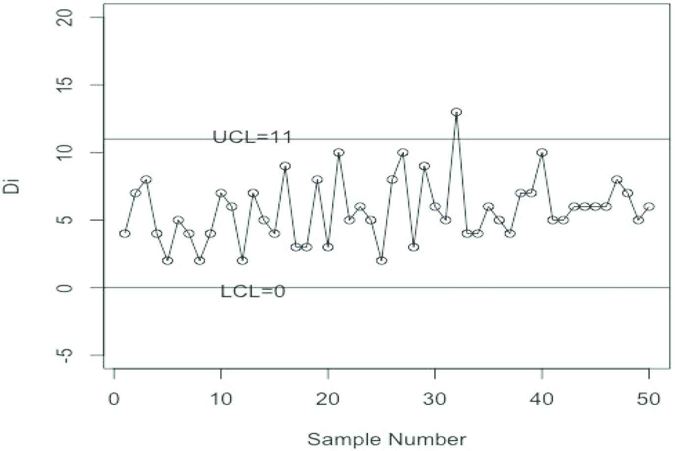
The proposed chart for simulation data.
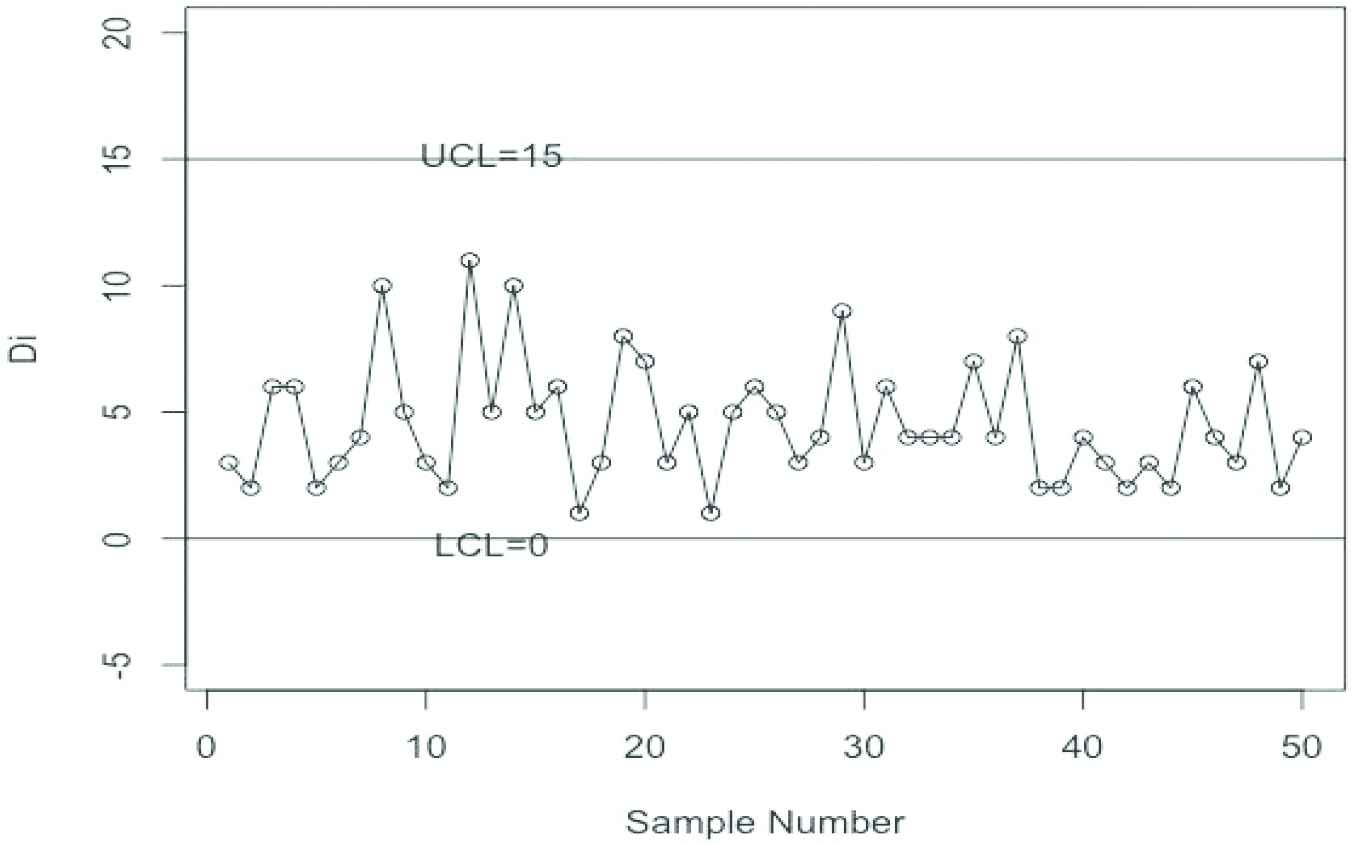
The [6] chart for simulation data.
4. ILLUSTRATIVE EXAMPLE
The proposed control chart was applied in an automobile manufacturing company located in South Korea. The company was interested in monitoring the service time in months for specific subsystems [6]. The same service data was applied by [6], who showed that the data followed the Weibull distribution with
3, 1, 4, 4, 3, 3, 3, 6, 4, 3, 5, 2, 3, 3, 4, 4, 4, 4, 6, 1, 4, 5, 5, 6, 7, 7, 2, 1, 7, 8, 3, 3, 3, 9, 4, 5, 10, 5, 5, 7.
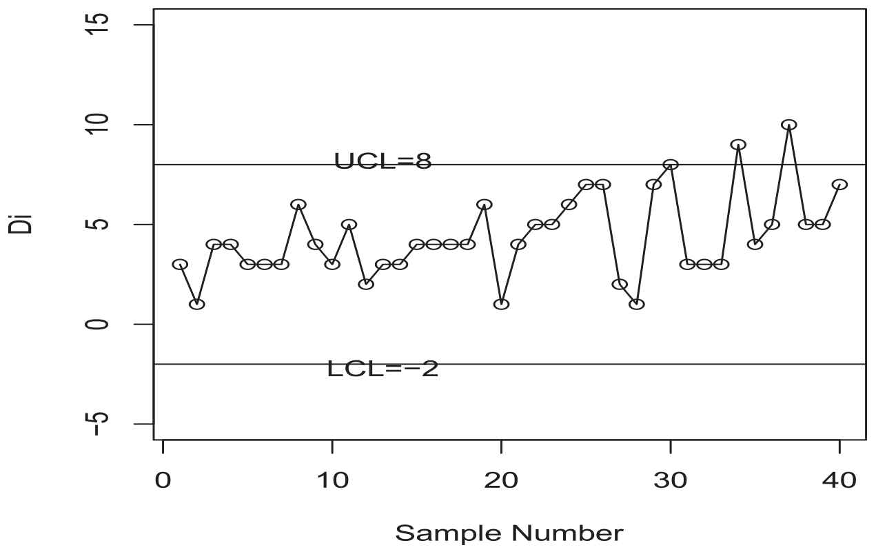
The proposed chart for real data.
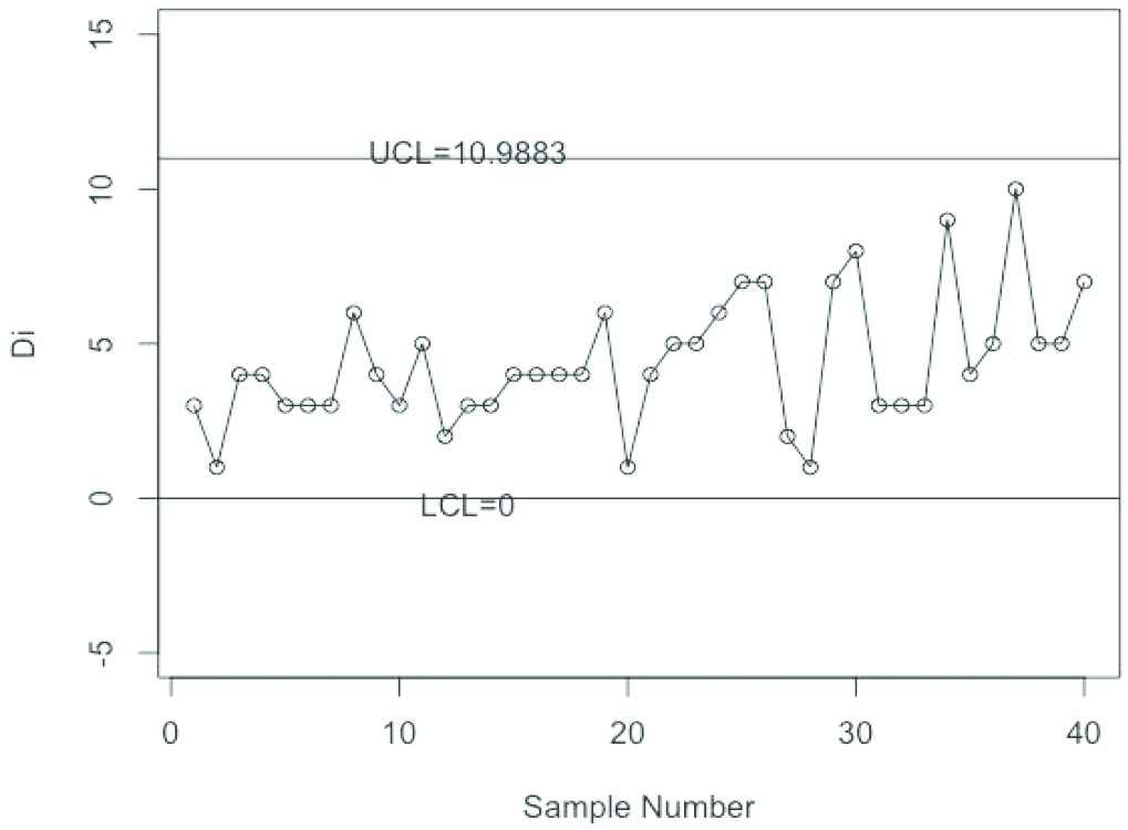
The existing chart for real data.
The control limits for the proposed chart are
5. CONCLUSIONS
The time-truncated attribute control chart was herein presented using the neutrosophic Weibull distribution. The measurement's indeterminacy effect was studied on the performance of the proposed control chart with the counterpart control chart. The proposed chart was the generalized version of the attribute control chart under a neutrosophic environment. From the results presented in Tables 1–4, we observed that the indeterminacy parameter significantly affected ARL values. The out-of-control ARL values reduced when indeterminacy increased. The comparative study proved the current chart's efficiency. The proposed control chart was proven to monitor service time in the automobile industry. The proposed control chart has limitations, i.e., it can only be applied when the life/service time follows the neutrosophic Weibull distribution. Secondly, the proposed control chart cannot be applied for variable data. The proposed control chart can be applied in the automobile industry, aircraft industry, and mobile industry for monitoring the defective items. In the future, the proposed control chart should be used for other neutrosophic statistical distributions. Following [7], the proposed control chart used an exponentially weighted moving average (EWMA) statistic and cumulative sum (CUSUM) statistic, both of which should be considered in future research.
CONFLICTS OF INTEREST
The authors declare no conflict of interest.
AUTHORS' CONTRIBUTIONS
A.H.A.M, A.S, M.A and A.A wrote the paper.
ACKNOWLEDGMENTS
The authors are deeply thankful to the editors and reviewers who offered invaluable suggestions for improving this manuscript. This article was supported by the Deanship of Scientific Research (DSR), King Abdulaziz University, Jeddah under project No. (G-22-130-1441). The authors, therefore, gratefully acknowledge the DSR technical and financial support.
REFERENCES
Cite this article
TY  - JOUR
AU  - Ali Hussein AL-Marshadi
AU  - Ambreen Shafqat
AU  - Muhammad Aslam
AU  - Abdullah Alharbey
PY  - 2021
DA  - 2021/04/06
TI  - Performance of a New Time-Truncated Control Chart for Weibull Distribution Under Uncertainty
JO  - International Journal of Computational Intelligence Systems
SP  - 1256
EP  - 1262
VL  - 14
IS  - 1
SN  - 1875-6883
UR  - https://doi.org/10.2991/ijcis.d.210331.001
DO  - 10.2991/ijcis.d.210331.001
ID  - AL-Marshadi2021
ER  -