A Hybrid Decision-Making Approach Under Complex Pythagorean Fuzzy N-Soft Sets

Muhammad Akram; Faiza Wasim; Ahmad N. Al-Kenani

doi:10.2991/ijcis.d.210331.002

<Previous Article In Issue

Download article (PDF)

Next Article In Issue>

Volume 14, Issue 1, 2021, Pages 1263 - 1291

A Hybrid Decision-Making Approach Under Complex Pythagorean Fuzzy N-Soft Sets

Authors

Muhammad Akram¹^{, *}^,, Faiza Wasim¹, Ahmad N. Al-Kenani²^,

¹Department of Mathematics, University of the Punjab, New Campus, Lahore, Pakistan

²Department of Mathematics, Faculty of Science, King Abdulaziz University, Jeddah, Saudi Arabia

^*Corresponding author. Email: m.akram@pucit.edu.pk

Corresponding Author

Muhammad Akram

Received 17 January 2021, Accepted 19 March 2021, Available Online 12 April 2021.

DOI: 10.2991/ijcis.d.210331.002 How to use a DOI?
Keywords: Complex Pythagorean fuzzy N-soft set; Einstein operations; MCDM; D-choice values of Pythagorean fuzzy N-soft set
Abstract: The main objectives of this article include the formal statement of a new mathematical model of uncertain knowledge and the presentation of its potential applications. The novel hybrid model is called complex Pythagorean fuzzy N-soft set (CPFNSS) because it enjoys both the parametric structure of N-soft sets and the most prominent features of complex Pythagorean fuzzy sets in order to capture the nuances of two-dimensional inexact information. We demonstrate that this model serves as a competent tool for ranking-based modeling of parameterized fuzzy data. We propose some basic set-theoretical operations on CPFNSSs and explore some of their practical properties. Furthermore, we elaborate the Einstein and algebraic operations on complex Pythagorean fuzzy N-soft values (CPFNSVs). We interpret its relationships with contemporary theories to vindicate the versatility of the proposed model. Moreover, we develop three algorithms to unfold the application of proposed theory in multi-criteria decision-making (MCDM). Some illustrative applications give a practical justification for these strategies. Finally, we conduct a comparative analysis of the performance of these algorithms with existing MCDM techniques, namely, choice values and D-choice values of Pythagorean fuzzy N-soft set (PFNSS), which validates the effectiveness of the proposed techniques.
Copyright: © 2021 The Authors. Published by Atlantis Press B.V.
Open Access: This is an open access article distributed under the CC BY-NC 4.0 license (http://creativecommons.org/licenses/by-nc/4.0/).

1. INTRODUCTION

Decision-making (DM) can be interpreted as a systematic process of solving real-world problems which provides an optimal solution after examining the feasible set of alternatives. DM approaches have gained popularity as they are widely used in various disciplines, including medical sciences, engineering, economics and many other areas of science and technology. Recently, the DM process has become more complex due to the presence of uncertainty and ambiguity in collected information which can bother the decision-makers to decide smoothly. The traditional DM strategies were powerless to deal with such uncertain and vague data. The pioneering solution to such problems was provided by Zadeh [53] by setting the foundations of fuzzy set (FS) theory in which each element is assigned by a membership degree lying between 0 and 1. Atanassov [11] generalized the idea of FS into intuitionistic fuzzy set (IFS) by adding nonmembership degree (λ) to the membership degree (μ) of FS, with the condition μ + λ ≤ 1. Yager [49,50] established the Pythagorean fuzzy set (PFS) theory, which relaxes the aforementioned condition of IFS to μ² + λ² ≤ 1. No doubt Pythagorean fuzzy expressions are raising the interest of many scholars, also in terms of their applications to DM. For example, Huang et al. [23] introduced a Pythagorean fuzzy MULTIMOORA method that uses a novel distance measure and a score function. They implemented this method for the evaluation of disk productions and energy projects. Akram et al. [6] have investigated risk evaluation in failure modes and effects analysis (FMEA) with the help of hybrid TOPSIS and ELECTRE I approaches under Pythagorean fuzzy information. Zhang and Xu [55] developed the TOPSIS method under Pythagorean fuzzy environment and implemented this method to evaluate the quality of private airline services. Zhou and Chen [56] presented the PF-TOPSIS method by utilizing a novel distance measure and illustrated its application for the commercialization of technology enterprises. Wang and Li [46] proposed a multi attribute DM method and power Bonferroni mean (PBM) operator for PF-information and applied this method to select the best online payment service providers. Wang and Chen [44] introduced the Pythagorean fuzzy LINMAP-based compromising method and elaborated the MCGDM problem for the selection of railway projects. Lin et al. [27] extended the TOPSIS method under the linguistic Pythagorean fuzzy environment by using a novel correlation coefficient and an entropy measure. They also highlighted some potential applications. Lin et al. [25] extended the TOPSIS and VIKOR methods for the probabilistic linguistic term information by using score function based on concentration degree. Lin et al. [26] put forward the directional correlation coefficient measures for Pythagorean fuzzy information and illustrated their potential applications in medical diagnosis and cluster analysis.

The theory of FSs and its generalizations were applied and explored by many researchers as they overcame the limitations of crisp set theory and served as precise tools to deal with specific types of imprecise data. However, these theories were not able to handle the inconsistent data of periodic nature until Ramot et al. [37] generalized the notion of FS by establishing a new theory of complex fuzzy sets (CFSs). In this theory the range of the membership function was extended from the unit interval to the unit disc of the complex plane. To overcome some deficiencies of CFS, Alkouri and Salleh [10] proposed the notion of complex intuitionistic fuzzy set (CIFS) by introducing complex-valued membership (μe^iα) and nonmembership (λe^iβ) degrees, in which the amplitude and phase terms are restricted by the conditions 0 ≤ μ + λ ≤ 1 and 0≤α2π+β2π≤1, respectively. Ullah et al. [43] broadened the space of CIFS by presenting the idea of complex Pythagorean fuzzy set (CPFS) and introduced new constraint conditions 0≤μ2+λ2≤1 and 0≤(α2π)2+(β2π)2≤1. The CPFS is an effective tool to capture the inconsistent data of periodic nature and it excels due to its relaxed conditions, excellent features and advantageous properties. This remarkable concept is extensively used in various territories including DM problems, networking, image processing, clustering, pattern recognition, engineering and many other fields of computer science. Lin et al. [29] introduced the linguistic q-rung orthopair FSs and their interactional partitioned Heronian mean aggregation operators. Wang and Garg [45] presented the multiple attribute DM approach by utilizing the interactive Archimedean norm operations and elaborated this method with the help of practical application.

The existing models such as FS [53], rough sets [34], CFS [37], CIFS [10] and CPFS [43] and many others, have been developed to capture various types of uncertainties and vagueness embedded in a system in an efficient way. However, all these theories have their own structure, impact, properties and inherent limitations. One major limitation of these models is the neglection of parametrization associated with these theories. To fix this problem, Molodtsov [33] established an entirely new theory of soft set (SS) which provides a parameterized mathematical framework relaxed from the above-stated limitations. The literature on soft set theory was further extended after observing its rich potential for practical applications in various directions. This theory soon attracted the attention of many researchers because it has been implemented in many areas of uncertainty such as mathematical analysis, forecasting, optimization theory, algebraic structures, information systems, data analysis and in DM applications. Yang et al. [52] introduced new fusion techniques under continuous interval-valued q-rung orthopair fuzzy environment and demonstrated its application for the selection of suitable SmartWatch design. Lin et al. [28] proposed integrated probabilistic linguistic multi-criteria decision-making (MCDM) method for the assessment of internet-of-things (IoT) programs. Rodríguez et al. [40] presented a novel consensus reaching process (CRP) model to capture the large-scale DM problems and applied it for intelligent CRP support system.

The development of soft set theory fascinated the researchers to amalgamate the soft set with other mathematical models. Peng et al. [35] proposed a generalization of soft set, namely, Pythagorean fuzzy soft set (PFSS) by fusing the soft set (SS) with PFS and interpreted this concept by some potential applications. Thirunavukarasu et al. [42] contributed to the literature by presenting the notion of complex fuzzy soft set (CFSS) and highlighting its applications. Kumar and Bajaj [24] put forward the complex intuitionistic fuzzy soft set (CIFSS) and discussed some entropies and distance measures. Lin et al. [30] proposed a new probability density based ordered weighted averaging (PDOWA) operator and demonstrated its application for the assessment of smart phones. Liu et al. [31,32] introduced hybrid models of long-term intertemporal hesitant fuzzy soft sets (LIT-HFSS) and hesitant linguistic expression soft sets (HLESS) along with significant group DM algorithms. Rodríguez et al. [39] proposed the comprehensive minimum cost models based on both distance measure and consensus degree to address the consistent fuzzy preference relations. Chen et al. [12] identified and prioritized the factors affecting the comfort of in-cabin passenger on fast-moving rail in China by using fuzzy linguistic group DM method.

In view of the theories stated above, it is clear that maximum research focus on the advanced models stimulated by soft sets was put on either its original binary interpretation (only 0 or 1 are allowed) or else real numbers within the unit interval [0, 1]. Despite of this, several daily life DM problems contain multinary but discrete type structured data. These multinary evaluations are frequently used in rating or ranking-based systems. In such systems, it is observed that ranking of alternatives such as hotels, websites, dramas, movies, music, games, magazines and books can be represented by a number of stars, dots, check marks, hearts, natural numbers and even by icons [9,16].

Obviously, this multinary parameterized data cannot be tackled by the above-mentioned soft set inspired models. Therefore, a different model was required in order to deal with such type of data. Motivated by all these facts, Fatimah et al. [16] developed the N-soft set (NSS) theory along with DM algorithms that emphasize the importance of ordered grades in practical examples. Later, Akram et al. [1,2] launched the advanced hybrid theories of hesitant N-soft set (HNSS) and fuzzy N-soft set (FNSS) by merging the concept of N-soft set with additional mathematical traits such as hesitancy and fuzziness of set, respectively. Akram et al. [3] combines all these features into hesitant fuzzy N-soft sets, and Akram et al. [4] introduced another hybrid model, namely, intuitionistic fuzzy N-soft set (IFNSS) by the suitable combination of N-soft sets with intuitionistic fuzzy expressions. Akram et al. [7] presented hesitant fuzzy N-soft ELECTRE-II model. Zhang et al. [54] developed the hybrid theory of Pythagorean fuzzy N-soft sets (PFNSSs) that merges the concepts of N-soft set and PFS. And Fatimah and Alcantud [15] have just presented the multi-fuzzy N-soft set model with applications to DM.

To summarize, the motivation of this article boils down to the following elements:

The idea of NSS captures the characterization of the universe of objects in a multinary parametric manner. Although this concept improves upon soft set theory, still it has no potential to handle the fuzziness of parameterized characterizations.
The CPFS theory tackles the uncertainty and periodicity of data at the same time, but it also has some deficiencies due to the inadequacy of parametrization.
Although the PFNSS model deals with imprecision in terms of multinary parameterized descriptions of the universe of objects, this tool is limited to model the fuzziness in just one dimension because of the lack of a phase term.
The concept of complex intuitionistic fuzzy N-soft set (CIFNSS) provides an effective model with a large ability to capture the vagueness of parameterized data. However it is restricted by the conditions 0≤μ+λ≤1 and 0≤α2π+β2π≤1.
The complex Pythagorean fuzzy soft set (CPFSS) theory presents a binary parameterized tool that copes with uncertainty and ambiguity of data with great generality. But this theory is unable to model the multinary framework of evaluations.

Motivated by all these concerns, this article introduces a novel mathematical hybrid model, namely, complex PFNSS. It merges the remarkable features of both CPFS and NSS theories. The proposed model is especially designed for ranking-based evaluations of two-dimensional parameterized DM problems. Moreover, the fundamental set-theoretic operations and significant properties of the proposed model are discussed. The relationships between the introduced model and existing models are brought to light. Then, Einstein operators and some other operations for complex Pythagorean fuzzy N-soft values (CPFNSVs) are designed and properly interpreted. With these techniques, three advanced DM algorithms are developed. Then, we illustrate their suitability with the help of some potential applications. Finally, a comparative analysis with existing methodologies is conducted in order to justify the reliability of the proposed strategies of solution.

In a nutshell, the main contributions of this article are:

This research article introduces a modern, productive and most general model abbreviated as complex Pythagorean fuzzy N-soft set (CPFNSS). It enables us to tackle the imprecision and periodicity of parameterized data having multinary but discrete structure.
The rationality and feasibility of the appropriate DM algorithms that benefit from this new framework is demonstrated with the help of some potential applications.
A comparative study with existing MCDM techniques, namely, choice values of PFNSS and D-choice values of PFNSS, validates the authenticity of the proposed techniques and justifies the consistency of the results.

This research article is structured as follows: Section 2 presents the preliminaries which include the fundamental definitions related to the CPFS, SS, NSS and PFNSS set. Section 3 introduces our new competent model and its basic set-theoretic operations. Further, it explores the relationships of proposed model with existing models. Section 4 investigates the Einstein and algebraic operations on CPFNSVs. Section 5 establishes three DMalgorithms and throws light on their application by the means of explanatory numerical examples for the selection of best laptop and plant location, respectively. Furthermore, Section 6 presents a comparison of our proposed techniques with existing MCDM techniques, namely, choice values of PFNSS and D-choice values of PFNSS. Finally, the purpose of Section 7 is to conclude this research article.

2. PRELIMINARIES

In this section, we present some elementary definitions required for the advanced developments.

Definition 2.1.

[43] Let Z be a universe of discourse. A CPFS Q on Z can be characterized as

Q={(z,μQ(z)eiαQ(z),λQ(z)eiβQ(z))z∈Z},

where i=−1, the amplitude terms μQ(z),λQ(z)∈[0,1] and phase terms αQ(z),βQ(z)∈[0,2π] satisfy the conditions 0≤μQ2(z)+λQ2(z)≤1 and 0≤(αΩ(z)2π)2+(βQ(z)2π)2≤1. For all z∈Z,χQ(z)=1−μQ2(z)−λQ2(z) ei2π1−(αO(z)2π)2−(βQ(z)2π)2 represents the degree of indeterminacy. The pair of membership and nonmembership degree (μQ(z)eiαQ(z),λQ(z)eiβQ(z)) is called a complex Pythagorean fuzzy number (CPFN).

Definition 2.2.

[33] Let Z be a universe of discourse and K be a set of parameters, S⊆K. A pair S=(F,S) is said to be a soft set over Z if F:S→P(Z), where P (Z) is the family of all subsets of Z. A soft set S over the universe Z can be represented as follows:

S={(sq,F(sq))sq∈S,F(sq)∈P(Z)}.

Definition 2.3.

[16] Let Z be a universe of discourse and K be a set of parameters. Let S⊆K and D={0,1,…,N−1} be a set of ordered grades with N∈{2,3,…}. A triplet L=(F,S,N) is called set on N-soft set on Z if F:S→2Z×D with the property that for each s∈S and z∈Z there exist a unique (z,ds)∈Z×D such that (z,ds)∈F(s),z∈Z,ds∈D. The N-soft set L over the universe Z can be represented as follows:

L={(sq,F(sq))sq∈S,F(sq)∈2Z×D}.

Definition 2.4.

[54] Let Z be a universe of discourse and K be a set of parameters. Let S⊆K and D={0,1,…,N−1} be a set of ordered grades with N∈{2,3,…}. A triple (f, L,N) is called a PFNSS on Z if L=(F,S,N) is NSS on Z and f:S→PFZ×D, where PFZ×D is the collection of all PFSs over Z × D. In other words, PFNSS (f,L,N) is defined as follows:

(f,L,N)={(sq,f(sq))sq∈S,f(sq)∈PFZ×D},

where f(sq)=((zp,dpq),μpq(zp,dpq),λpq(zp,dpq))(zp,dpq)∈Z×D represents the PFS over Z × D. The membership and nonmembership degrees μpqzp,dpq,λpqzp,dpq∈[0,1] satisfy the condition 0≤μpq2(zp,dpq)+ λpq2(zp,dpq)≤1. For all (zp,dpq)∈Z×D,χpq(zp,dpq)=1−μpq2(zp,dpq)−λpq2(zp,dpq) represents the degree of indeterminacy.

Definition 2.5.

[55] Let Y=(μY,λY) be a Pythagorean fuzzy number (PFN) over the universe of discourse Z. The score function and accuracy function of Y are defined as follows:

S(Y)=μY2−λY2 and A(Y)=μY2+λY2,(1)

where S(Y) belongs to the closed interval [−1, 1] and A(Y) belongs to the closed interval [0, 1].

For other terminologies and applications, the readers are referred to [5, 8, 13, 14, 17, 18, 19, 20, 21, 22, 36, 38, 41, 47, 48, 51].

3. COMPLEX PYTHAGOREAN FUZZY N-SOFT SET

Definition 3.1.

Let Z be a universe of discourse and K be a set of parameters. Let S ⊆ K and D = {0, 1, …, N − 1} be a set of ordered grades with N ∈ {2, 3, … }. A triplet Y = (h, L, N) is called a complex PFNSS on Z if L = (H, S, N) is NSS on Z and h: S → CPFZ×D, where CPFZ×D is the collection of all CPFSs over Z × D. The CPFNSS(h, L, N) can be defined as follows:

Y={⟨ sq,h(sq)⟩ sq∈S,h(sq)∈CPFZ×D},

where h(sq)=((zp,dpq),μpq(zp,dpq)eiαpq(zp,dpq),λpq(zp,dpq)eiβpq(zp,dpq))(zp,dpq)∈Z×D represents the CPFS over Z × D. The amplitude terms μ_pq(z_p, d_pq), λ_pq(z_p, d_pq) ∈ [0, 1] and phase returns α_pq(z_p, d_pq), β_pq(z_p,d_pq) ∈ [0, 2π] satisfy the conditions

0≤μpq2(zp,dpq)+λpq2(zp,dpq)≤1,0≤(αpq(zp,dpq)2π)2+(βpq(zp,dpq)2π)2≤1,

where i=−1. For all (z_p, d_pq) ∈ Z × D, the degree of indeterminacy is represented by χpq(zp,dpq)= 1−μpq2(zp,dpq)−λpq2(zp,dpq)ei2π1−(αpq(zp,dpq)2π)2−(βpq(zp,dpq)2π)2.

In other words, CPFNSS is a parameterized family of CPFSs of Z × D, that is, for each parameter s_q ∈ S, we can interpret that h(s_q) is the CPFS of Z × D.

Now, we give tabular representation of complex PFNSS:

Let Z be a set of r objects and S be a set of w attributes, then tabular representation of CPFNSS is given in Table 1.

(h, L, N)	s₁	s₂	…	s^ω
z₁	〈d₁₁,(μ₁₁e^{iα 11}, λ₁₁e^{iβ 11})〉	〈d₁₂,(μ₁₂e^{iα 12}, λ₁₂e^{iβ 12})〉	…	〈d_1ω,(μ_1ωe^{iα 1ω}, λ_1ωe^{iβ 1ω})〉
z₂	〈d₂₁,(μ₂₁e^{iα 21}, λ₂₁e^{iβ 21})〉	〈d₂₂,(μ₂₂e^{iα 22}, λ₂₂e^{iβ 22})〉	…	〈d_2ω,(μ_2ωe^{iα 2ω}, λ_2ωe^{iβ 2ω})〉
.	.	.	.	.
.	.	.	.	.
.	.	.	.	.
z_r	〈d_r1,(μ_r1e^{iα r1}, λ_r1e^{iβ r1})〉	〈d_r2,(μ_r2e^{iα r2}, λ_r2e^{iβ r2})〉	…	〈d_{r ω},(μ_{r ω}e^{iα r ω}, λ_{r ω}e^{iβ r ω})〉

Table 1

Tabular representation of CPFNSS.

Definition 3.2.

CPFNSS can be regarded as r × w table, where r = |Z|, w = |S| whose pqth element is called a complex Pythagorean fuzzy N-soft value (CPFNSV) and it has the form, τ_pq = 〈d_pq, (μ_pqe^iαpq, λ_pq^iβpq)〉, where p = 1, 2, …, r; q = 1, 2, …, w.

Definition 3.3.

The score function for CPFNSV, τ_pq = 〈d_pq, (μ_pqe^iαpq, λe^iβpq)〉 is represented by S and defined as follows:

S(τpq)=(dpqN−1)2+(μpq2−λpq2)+14π2(αpq2−βpq2),(2)

where S(τpq)∈[−2,3].

Definition 3.4.

The accuracy function for CPFNSV, τ_pq = 〈d_pq, (μ_pqe^iαpq, λ_pq^iβpq)〉 is represented by A and defined as follows:

A(τpq)=(dpqN−1)2+(μpq2+λpq2)+14π2(αpq2+βpq2),(3)

where A(τ_pq) ∈ [0, 3].

Definition 3.5.

Let τ₁₁ = 〈d₁₁, (μ₁₁e^iα11, λ₁₁^iβ11)〉 and τ₁₂ = 〈d₁₂, (μ₁₂e^iα12, λ₁₂^iβ12)〉 be any two CPFNSVs, then the comparison between τ₁₁ and τ₁₂ is defined as follows:

If S(τ11)<S(τ12), then τ11≺τ12 (τ₁₁ is inferior to τ₁₂);
If S(τ11)>S(τ12), then τ11≻τ12 (τ₁₁ is superior to τ₁₂);
If S(τ11)=S(τ12), then
- If A(τ11)<A(τ12), then τ11≺τ12 (τ₁₁ is inferior to τ₁₂);
- If A(τ11)>A(τ12), then τ11≻τ12 (τ₁₁ is superior to τ₁₂);
- If A(τ11)=A(τ12), then τ11~τ12 (τ₁₁ is equivalent to τ₁₂).

The significance and motivation of this proposed model is illustrated by the following numerical example. In order to develop intuition for this new concept, this example has been kept relatively simple. This simple example elaborates the difficulties of the existing Pythagorean fuzzy N-soft model, proposed by Zhang et al. [54] and demonstrates the competency of the proposed model in real-world DM problems.

Example 3.6.

A company wants to invest with another company to increase income. The selection of that company is determined by star rankings and ratings awarded by the experts of the selection panel. These ratings are based on the performance of companies in the last 12 months. Let Z = {z₁, z₂, z₃, z₄} be a collection of four companies and S = {s₁ = growth rate, s₂ = export, s₃ = interest rates} be a set of attributes which are used to assign ratings to companies.

A 5-soft set can be identified from Table 2, where

Four stars represent “Excellent,”
Three stars represent “Very Good,”
Two stars represent “Good,”
One star represents “Normal,”
Big dot represents “Poor.”

Z/S	s₁	s₂	s₃
z₁	⋆ ⋆ ⋆	⋆ ⋆ ⋆⋆	•
z₂	•	⋆ ⋆ ⋆	⋆
z₃	⋆	•	⋆ ⋆ ⋆⋆
z₄	⋆ ⋆ ⋆⋆	⋆⋆	⋆ ⋆ ⋆

Table 2

Rating of companies.

The numbers D = {0, 1, 2, 3, 4} can easily be associated with the graded evaluation carried out by stars as follows:

0 stands for “•,”
1 stands for “⋆,”
2 stands for “⋆ ⋆,”
3 stands for “⋆ ⋆ ⋆,”
4 stands for “⋆ ⋆ ⋆ ⋆.”

The rating of companies provided by the selection panel is given in Table 2.

Now, the tabular form of its corresponding 5-soft set is presented in Table 3.

(H, S, 5)	s₁	s₂	s₃
z₁	3	4	0
z₂	0	3	1
z₃	1	0	4
z₄	4	2	3

Table 3

5-soft set.

The selection panel thoroughly analyzes the companies to determine their rankings based on membership (μ) and nonmembership degrees (λ). So, we obtain Pythagorean fuzzy 5-soft set PF5SS, with the grading criteria followed by score degree of Pythagorean fuzzy number S(Ypq), where Ypq=(μpq,λpq), p = 1, 2, 3, 4, q = 1, 2, 3. This grading criteria is defined as follows:

−1.0≤S(Ypq)<−0.6when dpq=0,−0.6≤S(Ypq)<−0.2when dpq=1,−0.2≤S(Ypq)<0.2when dpq=2,0.2≤S(Ypq)<0.6when dpq=3,0.6≤S(Ypq)≤1.0when dpq=4.

According to above criteria, we can obtain Table 4 of grading criteria.

D	μ_pq	λ_pq
0	[0, 0.2)	(0.8, 1]
1	[0.2, 0.4)	(0.6, 0.8]
2	[0.4, 0.6)	(0.4, 0.6]
3	[0.6, 0.8)	(0.2, 0.4]
4	[0.8, 1]	[0, 0.2]

Table 4

Grading criteria.

Then, PF5SS is given as follows:

(hP,L,5)={(s1,h(s1)),(s2,h(s2)),(s3,h(s3))}, where

h(s1)={〈(z1,3),0.7,0.3〉,〈(z2,0),0.1,0.9〉,〈(z3,1),0.3,0.7〉,〈(z4,4),0.9,0.1〉},h(s2)={〈(z1,4),0.9,0.1〉,〈(z2,3),0.6,0.4〉,〈(z3,0),0.1,0.9〉,〈(z4,2),0.4,0.6〉},h(s3)={〈(z1,0),0.1,0.9〉,〈(z2,1),0.3,0.7〉,〈(z3,4),0.8,0.2〉,〈(z4,3),0.7,0.3〉}.

The tabular form of PF5SS is presented in Table 5.

(hP, L, 5)	s₁	s₂	o₃
z₁	〈3, (0.7, 0.3)〉	〈4, (0.9, 0.1)〉	〈0, (0.1, 0.9)〉
z₂	〈0, (0.1, 0.9)〉	〈3, (0.6, 0.4)〉	〈1, (0.3, 0.7)〉
z₃	〈1, (0.3, 0.7)〉	〈0, (0.1, 0.9)〉	〈4, (0.8, 0.2)〉
z₄	〈4, (0.9, 0.1)〉	〈2, (0.4, 0.6)〉	〈3, (0.7, 0.3)〉

Table 5

Pythagorean fuzzy 5-soft set.

The experts of the selection panel evaluate all the companies and assign membership and non-membership degrees μ(z, d), λ(z, d), respectively, to each company. Now, suppose an expert observes that “The growth rate of a company z₁ is high in the first 8 months but slightly declines in the last 4 months.” Then, the values of μ(z₁, 3) = 0.7, and λ(z₁, 3) = 0.3 are ambiguous and all the information regarding the time frame of reference would be lost. Thus μ(z₁, 3), λ(z₁, 3) can be assigned by complex values which incorporate all of the information provided by the expert. Hence, we establish complex Pythagorean fuzzy 5-soft set (CPF5SS) instead of Pythagorean fuzzy 5-soft set for the evaluation of such diﬃculty.

Now, the following value may, attributed to μ(z₁, 3) and λ(z₁, 3):

μ(z1,3)=0.7ei812⋅2π=0.7ei1.3π,λ(z1,3)=0.3ei412⋅2π=0.3ei0.6π.

Here, phase term represents the information regarding the time frame of reference under consideration. Therefore, CPF5SS (h, L, 5) is introduced by integrating CPFS with the 5-soft set for the two-dimensional graded evaluation of companies. Now, we redefine the grading criteria followed by score degree of CPF5SVs S(τpq), where τ_pq = 〈d_pq, (μ_pqe^iαpq, λ_pqe^iβpq)〉, p = 1, 2, 3, 4, q = 1, 2, 3 as follows:

−2.0≤S(τpq)<−1.0when dpq=0,−1.0≤S(τpq)<0.0when dpq=1, 0.0≤S(τpq)<1.0when dpq=2, 1.0≤S(τpq)<2.0when dpq=3, 2.0≤S(τpq)≤3.0when dpq=4.

According to above criteria, we can obtain Table 6 of corresponding redefined grading criteria.

Grades	Amplitude Terms		Phase Terms
D	μ_pq	λ_pq	α_pq	β_pq
0	[0, 0.2)	(0.8, 1]	[0π, 0.4π)	(1.6π, 2π]
1	[0.2, 0.4)	(0.6, 0.8]	[0.4π, 0.8π)	(1.2π, 1.6π]
2	[0.4, 0.6)	(0.4, 0.6]	[0.8π, 1.2π)	(0.8π, 1.2π]
3	[0.6, 0.8)	(0.2, 0.4]	[1.2π, 1.6π)	(0.4π, 0.8π]
4	[0.8, 1]	[0, 0.2]	[1.6π, 2π]	[0π, 0.4π]

Table 6

Redefined grading criteria.

Finally, CPF5SS is defined as follows:

(h,L,5)={(s1,h(s1)),(s2,h(s2)),(s3,h(s3))}, where

h(s1)=〈(z1,3),0.7ei1.3π,0.3ei0.6π〉,〈(z2,0),0.1ei0.1π,0.9ei1.9π〉,〈(z3,1),0.3ei0.7π,0.7ei1.4π〉,〈(z4,4),0.9ei1.7π,0.1ei0.3π〉,h(s2)=〈(z1,4),0.9ei1.7π,0.1ei0.3π〉,〈(z2,3),0.6ei1.2π,0.4ei0.8π〉,〈(z3,0),0.1ei0.3π,0.9ei1.8π〉,〈(z4,2),0.4ei0.8π,0.6ei1.2π〉,h(s3)=〈(z1,0),0.1ei0.2π,0.9ei1.9π〉,〈(z2,1),0.3ei0.5π,0.7ei1.3π〉,〈(z3,4),0.8ei1.6π,0.2ei0.4π〉,〈(z4,3),0.7ei1.3π,0.3ei0.7π〉.

Clearly, CPF5SS can be represented in tabular form by Table 7.

(h, L, 5)	s₁	s₂	s₃
z₁	〈3, (0.7e^i1.3π, 0.3e^i0.6π)〉	〈4, (0.9e^i1.7π, 0.1e^i0.3π)〉	〈0, (0.1e^i0.2π, 0.9e^i1.9π)〉
z₂	〈0, (0.1e^i0.1π, 0.9e^i1.9π)〉	〈3, (0.6e^i1.2π, 0.4e^i0.8π)〉	〈1, (0.3e^i0.5π, 0.7e^i1.3π)〉
z₃	〈1, (0.3e^i0.7π, 0.7e^i1.4π)〉	〈0, (0.1e^i0.3π, 0.9e^i1.8π)〉	〈4, (0.8e^i1.6π, 0.2e^i0.4π)〉
z₄	〈4, (0.9e^i1.7π, 0.1e^i0.3π)〉	〈2, (0.4e^i0.8π, 0.6e^i1.2π)〉	〈3, (0.7e^i1.3π, 0.3e^i0.7π)〉

Table 7

Tabular representation of CPF5SS.

Remark 3.7.

Any CPF2SS (h, L, 2) can be naturally identified with CPFSS. We associate CPF2SS h: S → 2^Z×{0,1} with CPFSS h^′: S → CPF(Z), which is defined by
h′(sq)={(zp,μpq(zp)eiαpq(zp),λpq(zp)eiβpq(zp))〈((zp,1),μpq(zp,1)eiαpq(zp,1),λpq(zp,1)eiβpq(zp,1))〉∈h(sq)},
for every s_q ∈ S.
A CPFNSS (h, L, N) on a nonempty set Z is said to be efficient if 〈(z_p, N − 1), μ(z_p, N − 1)e^{iα(zp,N − 1)}, λ(z_p, N − 1)e^{iβ(_zp, N − 1)}〉 ∈ h(s_q), for some s_q ∈ S, z_p ∈ Z.
Grade 0 ∈ D in Definition 3.1, represents the lowest score. It does not mean that there is incomplete information or lack of assessment.

We now explore the conception of complementarity of Complex PFNSSs.

Definition 3.8.

Let (h, L, N) be a CPFNSS over the universe Z, where L = (H, S, N) is the NSS on Z. Then, its Complex Pythagorean fuzzy complement (h^c, L, N) is defined as

(hc,L,N)={〈sq,hc(sq)〉sq∈S,hc(sq)∈CPFZ×D},where

hc(sq)={〈(zp,dpq),λ(zp,dpq)eiβ(zp,dpq),μ(zp,dpq)eiα(zp,dpq)〉(zp,dpq)∈Z×D}.

Definition 3.9.

Let (h, L, N) be a CPFNSS over the universe Z, where L = (H, S, N) be the NSS on Z. Then, its weak complex Pythagorean fuzzy complement (h^c, L^c, N) can be interpreted as

(hc,Lc,N)={⟨ sq,hc(sq)⟩ sq∈S,hc(sq)∈CPFZ×D},

where hc(sq)={〈(zp,dpq),λ(zp,dpq)eiβ(zp,dpq),μ(zp,dpq)eiα(zp,dpq)〉(zp,dpq)∈Z×D} and for all s_q ∈ S, H^c(s_q) ∩ H(s_q) = ϕ.

Example 3.10.

Consider the CPF5SS as defined in Example 3.6. Then, its complex Pythagorean fuzzy complement (h^c, L, 5) and weak complex Pythagorean fuzzy complement (h^c, L^c, 5) are given by Tables 8 and 9, respectively.

(h^c, L, 5)	s₁	s₂	s₃
z₁	〈3, (0.3e^i0.7π, 0.7e^i1.3π)〉	〈4, (0.1e^i0.3π, 0.9e^i1.7π)〉	〈0, (0.9e^i1.9π, 0.1e^i0.2π)〉
z₂	〈0, (0.9e^i1.9eπ, 0.1e^i0.1π)〉	〈3, (0.4e^i0.8π, 0.6e^i1.2π)〉	〈1, (0.7e^i1.3eπ, 0.3e^i0.5π)〉
z₃	〈1, (0.7e^i1.4π, 0.3e^i0.7π)〉	〈0, (0.9e^i1.8π, 0.1e^i0.3π)〉	〈4, (0.2e^i0.4π, 0.8e^i1.6π)〉
z₄	〈4, (0.1e^i0.3π, 0.9e^i1.7π)〉	〈2, (0.6e^i1.2π, 0.4e^i0.8π)〉	〈3, (0.3e^i0.7π, 0.7e^i1.3π)〉

Table 8

Complex Pythagorean fuzzy complement.

(h^c, L^c, 5)	s₁	s₂	s₃
z₁	〈1, (0.3e^i0.7π, 0.7e^i1.3π)〉	〈2, (0.1e^i0.3π, 0.9e^i1.7π)〉	〈1, (0.9e^i1.9π, 0.1e^i0.2π)〉
z₂	〈4, (0.9e^i1.9π, 0.1e^i0.1π)〉	〈4, (0.4e^i0.8π, 0.6e^i1.2π)〉	〈3, (0.7e^i1.3π, 0.3e^i0.5π)〉
z₃	〈0, (0.7e^i1.4π, 0.3e^i0.7π)〉	〈1, (0.9e^i1.8π, 0.1e^i0.3π)〉	〈2, (0.2e^i0.4π, 0.8e^i1.6π)〉
z₄	〈2, (0.1e^i0.3π, 0.9e^i1.7π)〉	〈3, (0.6e^i1.2π, 0.4e^i0.8π)〉	〈4, (0.3e^i0.7π, 0.7e^i1.3π)〉

Table 9

Weak complex Pythagorean fuzzy complement.

Definition 3.11.

Let (h, L, N) be a CPFNSS over the universe Z, where L = (H, S, N) is the NSS on Z. Then, its top complex Pythagorean fuzzy weak complement, denoted by (h^t, L^t, N) is defined as

(ht,Lt,N)={ht(sq)=〈(zp,N−1),λ(zp,dpq)eiβ(zp,dpq),μ(zp,dpq)eiα(zp,dpq)〉,if dpq<N−1ht(sq)=〈(zp,0),λ(zp,dpq)eiβ(zp,dpq),μ(zp,dpq)eiα(zp,dpq)〉,if dpq=N−1(4)

Definition 3.12.

Let (h, L, N) be a CPFNSS over the universe Z, where L = (H, S, N) is the NSS on Z. Then, its bottom complex Pythagorean fuzzy weak complement, denoted by (h^b, L^b, N) is defined as

(hb,Lb,N)={hb(sq)=〈(zp,0),λ(zp,dpq)eiβ(zp,dpq),μ(zp,dpq)eiα(zp,dpq)〉,if dpq>0,hb(sq)=〈(zp,N−1),λ(zp,dpq)eiβ(zp,dpq),μ(zp,dpq)eiα(zp,dpq)〉,if dpq=0.(5)

Example 3.13.

Consider the CPF5SS as defined in Example 3.6. Then, its top complex Pythagorean fuzzy weak complement (h^t, L^t, 5) and bottom complex Pythagorean fuzzy weak complement (h^b, L^b, 5) are given by Tables 10 and 11, respectively.

(h^t, L^t, 5)	s₁	s₂	s₃
z₁	〈4, (0.3e^i0.7π, 0.7e^i1.3π)〉	〈0, (0.1e^i0.3π, 0.9e^i1.7π)〉	〈4, (0.9e^i1.9π, 0.1e^i0.2π)〉
z₂	〈4, (0.9e^i1.9π, 0.1e^i0.1π)〉	〈4, (0.4e^i0.8π, 0.6e^i1.2π)〉	〈4, (0.7e^i1.3π, 0.3e^i0.5π)〉
z₃	〈4, (0.7e^i1.4π, 0.3e^i0.7π)〉	〈4, (0.9e^i1.8π, 0.1e^i0.3π)〉	〈0, (0.2e^i0.4π, 0.8e^i1.6π)〉
z₄	〈0, (0.1e^i0.3π, 0.9e^i1.7π)〉	〈4, (0.6e^i1.2π, 0.4e^i0.8π)〉	〈4, (0.3e^i0.7π, 0.7e^i1.3π)〉

Table 10

Top complex Pythagorean fuzzy weak complement.

(h^b, L^b, 5)	s₁	s₂	s₃
z₁	〈0, (0.3e^i0.7π, 0.7e^i1.3π)〉	〈0, (0.1e^i0.3π, 0.9e^i1.7π)〉	〈4, (0.9e^i1.9π, 0.1e^i0.2π)〉
z₂	〈4, (0.9e^i1.9π, 0.1e^i0.1π)〉	〈0, (0.4e^i0.8π, 0.6e^i1.2π)〉	〈0, (0.7e^i1.3π, 0.3e^i0.5π)〉
z₃	〈0, (0.7e^i1.4π, 0.3e^i0.1π)〉	〈4, (0.9e^i1.8π, 0.1e^i0.3π)〉	〈0, (0.2e^i0.4π, 0.8e^i1.6π)〉
z₄	〈0, (0.1e^i0.3π, 0.9e^i1.7π)〉	〈0, (0.6e^i1.2π, 0.4e^i0.8π)〉	〈0, (0.3e^i0.7π, 0.7e^i1.3π)〉

Table 11

Bottom complex Pythagorean fuzzy weak complement.

Definition 3.14.

Let (h₁, L₁, N₁) and (h₂, L₂, N₂) be two CPFNSSs over the universe Z, where L₁ = (H₁, A, N₁) and L₂ = (H₂, B, N₂) are NSSs on Z. Then, their restricted intersection denoted by (h₁, L₁, N₁)∩_R(h₂, L₂, N₂) = (g, L₁ ∩_R L₂, min(N₁, N₂)), where L₁ ∩_R L₂ = (G, A ∩ B, min(N₁, N₂)) is defined as

∀s_q ∈ A ∩ B, z_p ∈ Z, 〈(zp,dpq),x,y〉∈g(sq)⇔dpq=min(dpq1,dpq2), x=min(μC(zp,dpq1),μD(zp,dpq2)), eimin(αC(zp,dpq1),αD(zp,dpq2)),y=max(λC(zp,dpq1),λD(zp,dpq2))eimax(βC(zp,dpq1),βD(zp,dpq2)), if 〈(zp,dpq1),μC(zp,dpq1) eiαC(zp,dpq1),λC(zp,dpq1)eiβC(zp,dpq1)〉 ∈h1(sq) and 〈(zp,dpq2),μD(zp,dpq2)eiαD(zp,dpq2),λD(zp,dpq2)eiβD(zp,dpq2)〉 ∈h2(sq), C and D are CPFSs on H₁(s_q) and H₂(s_q), respectively.

Definition 3.15.

Let (h₁, L₁, N₁) and (h₂, L₂, N₂) be two CPFNSSs over the universe Z, where L₁ = (H₁, A, N₁) and L₂ = (H₂, B, N₂) are NSSs on Z. Then, their extended intersection denoted by (h₁, L₁, N₁)∩_ε (h₂, L₂, N₂) = (f, L₁ ∩_εL₂, max(N₁, N₂)), where L₁ ∩_EL₂ = (F, A ∪ B, max(N₁, N₂)) is defined as

f(sq)={h1(sq),if sq∈A−Bh2(sq),if sq∈B−A〈(zp,dpq),x,y〉,such that dpq=min(dpq1,dpq2) x=min(μC(zp,dpq1),μD(zp,dpq2))eimin(αC(zp,dpq1),αD(zp,dpq2)) y=max(λC(zp,dpq1),λD(zp,dpq2))eimax(βC(zp,dpq1),βD(zp,dpq2)) where 〈(zp,dpq1),μC(zp,dpq1)eiαC(zp,dpq1),λC(zp,dpq1)eiβC(zp,dpq1)〉∈h1(sq) and 〈(zp,dpq2),μD(zp,dpq2)eiαD(zp,dpq2),λD(zp,dpq2)eiβD(zp,dpq2)〉∈h2(sq), C and D are CPFSs on H1(sq) and H2(sq), respectively.

Example 3.16.

Consider the tabular form of CPF6SS (h₁, L₁, 6) and CPF4SS (h₂, L₂, 4) as given in Tables 12 and 13, respectively, where L₁ = (H₁, A, 6), L₂ = (H₂, B, 4) are 6-soft set and 4-soft set over Z, respectively. Then, their restricted intersection (g, L₁ ∩_R L₂, 4) and extended intersection (f, L₁ ∩_ε L₂, 6) are presented in Tables 14 and 15, respectively.

(h₁, L₁, 6)	s₁	s₂	s₃
z₁	〈3, (0.59e^i1.23π, 0.42e^i0.78π)〉	〈4, (0.76e^i1.45π, 0.32e^i0.66π)〉	〈3, (0.61e^i1.30π, 0.48e^i0.88π)〉
z₂	〈5, (0.95e^i1.82π, 0.14e^i0.12π)〉	〈2, (0.43e^i0.66π, 0.64e^i1.32π)〉	〈0, (0.15e^i0.28π, 0.85e^i1.88π)〉
z₃	〈1, (0.26e^i0.33π, 0.82e^i1.65π)〉	〈0, (0.12e^i0.29π, 0.92e^i1.78π)〉	〈1, (0.28e^i0.51π, 0.81e^i1.45π)〉
z₄	〈4, (0.73e^i1.45π, 0.32e^i0.66π)〉	〈5, (0.85e^i1.78π, 0.12e^i1.30π)〉	〈2, (0.41e^i0.81π, 0.62e^i1.12π)〉

Table 12

CPF6SS.

(h₂, L₂, 4)	s₁	s₂	s₄
z¹	〈2, (0.65e^i1.25π, 0.41e^i0.85π)〉	〈3, (0.85e^i1.85π, 0.35e^i0.46π)〉	〈1, (0.35e^i0.5π, 0.61e^i1.50π)〉
z₂	〈1, (0.41e^i0.82π, 0.71e^i1.29π)〉	〈2, (0.55e^i1.45π, 0.15e^i0.62π)〉	〈0, (0.21e^i0.12π, 0.85e^i1.62π)〉
z₃	〈0, (0.91e^i0.42π, 0.82e^i1.81π)〉	〈1, (0.45e^i0.71π, 0.65e^i1.44π)〉	〈3, (0.92e^i1.92π, 0.12e^i0.43π)〉
z₄	〈3, (0.81e^i1.68π, 0.21e^i0.12π)〉	〈0, (0.14e^i0.14π, 0.98e^i1.92π)〉	〈2, (0.71e^i1.34π, 0.41e^i0.71π)〉

Table 13

CPF6SS.

(g,L1∩RL2,4)	s₁	s₂
z₁	〈2, (0.59e^i1.23π, 0.42e^i0.85π)〉	〈3, (0.76e^i1.45π, 0.35e^i0.66π)〉
z₂	〈1, (0.41e^i0.82π, 0.71e^i1.29π)〉	〈2, (0.43e^i0.66π, 0.64e^i1.32π)〉
z₃	〈0, (0.91e^i0.33π, 0.82e^i1.81π)〉	〈0, (0.12e^i0.29π, 0.92e^i1.78π)〉
z₄	〈3, (0.73e^i1.45π, 0.32e^i0.66π)〉	〈0, (0.14e^i0.14π, 0.98e^i1.92π)〉

Table 14

Restricted intersection.

(f,L1∩εL2,6)	s₁	s₂	s₃	s₄
z₁	〈2, (0.59e^i1.23π, 0.42e^i0.85π)〉	〈3, (0.76e^i1.45π, 0.35e^i0.66π)〉	〈3, (0.61e^i1.30π, 0.48e^i0.88π)〉	〈1, (0.35e^i0.50π, 0.61e^i1.50π)〉
z²	〈1, (0.41e^i0.82π, 0.71e^i1.29π)〉	〈2, (0.43e^i1.66π, 0.64e^i1.32π)〉	〈0, (0.15e^i0.28π, 0.85e^i1.88π)〉	〈0, (0.21e^i0.12π, 0.85e^i1.62π)〉
z³	〈0, (0.19e^i0.33π, 0.82e^i1.81π)〉	〈0, (0.12e^i0.29π, 0.92e^i1.78π)〉	〈1, (0.28e^i0.51π, 0.81e^i1.45π)〉	〈3, (0.92e^i1.92π, 0.12e^i0.43π)〉
z⁴	〈3, (0.73e^i1.45π, 0.32e^i0.66π)〉	〈0, (0.14e^i0.14π, 0.98e^i1.92π)〉	〈2, (0.41e^i0.81π, 0.62e^i1.12π)〉	〈2, (0.71e^i1.34π, 0.41e^i0.71π)〉

Table 15

Extended intersection.

Definition 3.17.

Let (h₁, L₁, N₁) and (h₂, L₂, N₂) be two CPFNSSs over the universe Z, where L₁ = (H₁, A, N₁) and L₂ = (H₂, B, N₂) are NSSs on Z. Then, their restricted union denoted by (h₁, L₁, N₁) ∪_R (h₂, L₂, N₂) = (w, L₁ ∪_RL₂, max(N₁, N₂)), where L₁ ∪_RL₂ = (W, A ∩ B, max(N₁, N₂)) is defined as

for all s_q ∈ A ∩ B, z_p ∈ Z, 〈(z_p, d_pq), x, y〉 ∈ w(s_q) ⇔ d_pq dpq=max(dpq1,dpq2), x=max(μC(zp,dpq1),μD(zp,dpq2))eimax(αC(zp,dpq1),αD(zp,dpq2)),y=min(λC(zp,dpq1),λD(zp,dpq2))eimin(βC(zp,dpq1),βD(zp,dpq2)), if 〈(zp,dpq1),μC(zp,dpq1) eiαC(zp,dpq1),λC(zp,dpq1)eiβC(zp,dpq1)〉 ∈h1(sq) and 〈(zp,dpq2),μD(zp,dpq2)eiαD(zp,dpq2),λD(zp,dpq2)eiβD(zp,dpq2)〉 ∈h2(sq) C and D are CPFSs on H₁(sq) and H₂(sq), respectively.

Definition 3.18.

Let (h₁, L₁, N₁) and (h₂, L₂, N₂) be two CPFNSSs over the universe Z, where L₁ = (H₁, A, N₁) and L₂ = (H₂, B, N₂) are NSSs on Z. Then, their extended union denoted by (h₁, L₁, N₁) ∪_E (h₂, L₂, N₂) = (z, L₁ ∪_εL₂, max(N₁, N₂)), where L₁ ∪_εL₂ = (Z, A ∪ B, max(N₁, N₂)) is defined as

z(sq)={h1(sq),if sq∈A−B,h2(sq),if sq∈B−A,〈(zp,dpq),x,y〉,such that dpq=max(dpq1,dpq2), x=max(μC(zp,dpq1),μD(zp,dpq2))eimax(αC(zp,dpq1),αD(zp,dpq2)), y=min(λC(zp,dpq1),λD(zp,dpq2))eimin(βC(zp,dpq1),βD(zp,dpq2)), where 〈(zp,dpq1),μC(zp,dpq1)eiαC(zp,dpq1),λC(zp,dpq1)eiβC(zp,dpq1)〉∈h1(sq), and 〈(zp,dpq2),μD(zp,dpq2)eiαD(zp,dpq2),λD(zp,dpq2)eiβD(zp,dpq2)〉∈h2(sq), C and D are CPFSs on H1(sq) and H2(sq), respectively.

Example 3.19.

Consider the CPF6SS and CPF4SS as given in Example 3.16. Then, their restricted union (w, L₁ ∪_R L₂, 6) and extended union (z, L₁ ∪_εL₂, 6) are presented in Tables 16 and 17, respectively.

(w,L1∪RL2,6)	s₁	s₂
z₁	〈3, (0.65e^i1.25π, 0.41e^i0.78π)〉	〈4, (0.85e^i1.85π, 0.32e^i0.46π)〉
z₂	〈5, (0.95e^1.82π, 0.14e^i0.12π)〉	〈2, (0.55e^1.45π, 0.15e^i0.62π)〉
z₃	〈1, (0.26e^i0.42π, 0.82e^i1.65π)〉	〈1, (0.45e^i0.71π, 0.65e^i1.44π)〉
z₄	〈4, (0.81e^i1.68π, 0.21e^i0.12π)〉	〈5, (0.85e^i1.78π, 0.12e^i0.30π)〉

Table 16

Restricted union.

(z,L1∪εL2,6)	s₁	s₂	s₃	s₄
z₁	〈3, (0.65e^i1.25π, 0.41e^i0.78π)〉	〈4, (0.85e^i1.85π, 0.32e^i0.46π)〉	〈3, (0.61e^i1.30π, 0.48e^i0.88π)〉	〈1, (0.35e^i0.50π, 0.61e^i1.50π)〉
z₂	〈5, (0.95e^i1.82π, 0.14e^i0.12π)〉	〈2, (0.55e^i1.45π, 0.15e^i0.62π)〉	〈0, (0.15e^i0.28π, 0.85e^i1.88π)〉	〈0, (0.21e^i0.12π, 0.85e^i1.62π)〉
z₃	〈1, (0.26e^i0.42π, 0.82e^i1.65π)〉	〈1, (0.45e^i0.71π, 0.65e^i1.44π)〉	〈1, (0.28e^i0.51π, 0.81e^i1.45π)〉	〈3, (0.92e^i1.92π, 0.12e^i0.43π)〉
z₄	〈4, (0.81e^i1.68π, 0.21e^i0.12π)〉	〈5, (0.85e^i1.78π, 0.12e^i0.30π) 〉	〈2, (0.41e^i0.81π, 0.62e^i1.12π)〉	〈2, (0.71e^i1.34π, 0.41e^i0.71π)〉

Table 17

Extended union.

Remark 3.20.

The Definitions 3.14, 3.15, 3.17, and 3.18 of restricted(or extended) intersection and union will satisfy the grading criteria if and only if N₁ = N₂

The concept of CPFNSS can be related to extant theories including complex PFSS, PFNSS, N-soft set and soft set. We shall establish all these relationships in this section. In order to derive CPFSS and SS from CPFNSS, we use the following definitions:

Definition 3.21.

Let (h, L, N) be a CPFNSS over a universe of discourse Z, where L = (H, S, N) is the NSS on Z. Let 0 < T < N be a threshold. Then, CPFSS over Z associated with (h, L, N) and T denoted by (h^T, S) is defined as follows:

hT(sq)={〈μpqeiαpq,λpqeiβpq〉,if〈dpq,(μpqeiαpq,λpqeiβpq)〉∈h(sq)anddpq≥T,{〈0.0ei0.0π,0.5ei1.0π〉,ifdpqN≥0.5〈0.0ei0.0π,1.0ei2.0π〉,ifdpqN<0.5.

Specifically, (h¹, S) is said to be bottom CPFSS and (h^N−1, S) is said to be top CPFSS associated with CPFNSS.

Definition 3.22.

Let 0 < T < N and ρ ∈ [−2, 2] be thresholds. The soft set over Z associated with (h, L, N) and (T, ρ), denoted by (h^{(T, ρ)}, S) is defined by the assignment:

h(T,ρ)(sq)={z∈Z:S(hT(sq))>ρ}, for each sq∈S

where S(hT(sq)) is the score function of hT(sq)=〈μpqTeiαpqT,λpqTeiβpqT〉.

Example 3.23.

Consider the CPF5SS (h, L, 5), represented by Table 7. We have 0 < T < 5, from Definition 3.21. The CPFSS associated with threshold T = 2 is given by Table 18. Meanwhile, while taking (T, ρ) = (3, 0.2), we can obtain the soft set (h^(3,0.2), S) which is given in Table 19.

(h², S)	s₁	s₂	s₃
z₁	〈0.7e^i1.3π, 0.3e^i0.7π〉	〈0.97e^i1.7π, 0.1e^i0.3π〉	〈0.0e^i0.0π, 1.0e^i2.0π〉
z₂	〈0.0e^i0.0π, 1.0e^i2.0π〉	〈0.6e^i0.0π, 0.4e^i2.0π〉	〈0.0e^i0.0π, 1.0e^i2.0π〉
z₃	〈0.0e^i0.0π, 1.0e^i2.0π〉	〈0.0e^i0.0π, 1.0e^i2.0π〉	〈0.8e^i1.6π, 0.2e^i0.4π〉
z₄	〈0.9e^i1.7π, 0.1e^i0.3π〉	〈0.4e^i0.8π, 0.6e^i1.2π〉	〈0.7e^i1.3π, 0.3e^i0.7π〉

Table 18

CPFSS associated with (h, L, 5) and threshold T = 2.

(h^(3,0.2), S)	s₁	s₂	s₃
z₁	1	1	0
z₂	0	1	0
z₃	0	0	1
z₄	1	0	1

Table 19

SS associated with (h, L, 5) and thresholds T = 3, ρ = 0.2.

In view of above analysis, it is observed that CPFNSS can be converted into CPFSS and SS under certain conditions. In other words, CPFNSS is the generalization of CPFSS and SS.

Remark 3.24.

Let Z be a universe of discourse, K be a set of parameters and S ⊆ K. Let (h, L, N) be a CPFNSS on Z. Then, the NSS associated with CPFNSS (h, L, N) is L, where L = (H, S, N).

This simple assignment shows that CPFNSS generalizes NSS, therefore SS as well.
Every complex intuitionistic fuzzy N-soft set (CIFNSS) is also a CPFNSS but converse is not true, because,
- If 0 ≤ μ + λ ≤ 1, then 0 ≤ μ² + λ² ≤ 1, for all μ, λ ∈ [0, 1].
- If 0 ≤ α + β ≤ 2π, then 0 ≤ (α2π)2 + (β2π)2 ≤ 1, for all α, β ∈ [0, 2π].
This implies that CPFNSS generalizes the CIFNSS.
CPFNSS is also a PFNSS when both phase terms of membership and nonmembership degrees are zero, that is, when α_pq = 0 = β_pq in Definition 3.1, we get the definition of PFNSS which is given as follows:
(h,L,N)={⟨ sq,h(sq)|sq∈S,h(sq)∈PFSZ×D},
where h(s_q) = {((z_q, d_pq), μ_pq(z_q, d_pq), λ_pq(z_q, d_pq)|(z_q, d_pq) ∈ Z × D} represents the PFS and PFSZ×D be the family of all PFSs over Z × D

Also, it is known that PFNSSs generalize the IFNSSs, FNSSs, NSSs, SSs, PFSSs and IFSSs. Therefore, we can also claim that CPFNSSs generalize all those models.

4. OPERATIONS

We now present operations on complex Pythagorean fuzzy N-soft values.

Definition 4.1.

Let τ1q=〈d1q,(μ1qeiα1q,λ1qeiβ1q)〉 (q=1,2), and τ = 〈d, (μe^iα, λe^iβ)〉 be any three CPFNSVs and Ω > 0 be any real number. Then, the following operations are defined over CPFNSVs as follows:

τ11⊕τ12=〈max(d11,d12),(μ112+μ122−μ112μ122 ei2π(α112π)2+(α122π)2−(α112π)2(α122π)2, λ11λ12ei2π(β112πβ122π))〉;
τ11⊗τ12=〈min(d11,d12),(μ11μ12ei2π(α112πα122π), λ112+λ122−λ112λ122 ei2π(β112π)2+(β122π)2−(β112π)2(β122π)2)〉;
Ωτ=〈d,(1−(1−μ2)Ω ei2π1−(1−(α2π)2)Ω, λΩei2π(β2π)Ω) 〉;
τΩ=〈d,(μΩei2π(α2π)Ω, 1−(1−λ2)Ω ei2π1−(1−(β2π)2)Ω)〉.

Definition 4.2.

Consider any three CPFNSVs, τ=〈d,(μeiα,λeiβ)〉,τ1q=〈1q,(μ1qeiα1q,λ1qeiβ1q)〉 (q = 1, 2) and Ω > 0 be any real number. Then, the following Einstein operations are defined over CPFNSVs as follows:

τ11⊕eτ12= 〈max(d11,d12) , (μ112+μ1221+μ112μ122e i2π(α112π)2+(α122π)21+(α112π)2(α122π)2, λ11λ121+(1−λ112)(1−λ122)ei2π(β112π)(β122π)1+(1−(β112π)2)(1−(β122π)2))〉;
τ11⊕eτ12= 〈min(d11,d12) , (μ11μ121+(1−μ112)(1−μ122)ei2π(α112π)(α122π)1+(1−(α112π)2)(1−(α122π)2),λ112+λ1221+λ112λ122ei2π(β112π)2+(β122π)21+(β112π)2(β122π)2 )〉;
Ω⋅eτ= 〈d, ((1+μ2)Ω−(1−μ2)Ω(1+μ2)Ω+(1−μ2)Ωe i2π(1+(α2π)2)Ω−(1−(α2π)2)Ω(1+(α2π)2)Ω+(1−(α2π)2)Ω , 2λΩ(2−λ2)Ω+(λ2)Ωe i2π2(β2π)Ω(2−(β2π)2)Ω+((β2π)2)Ω)〉;
τΩ= 〈d,(2μΩ(2−μ2)Ω+(μ2)Ωei2π2(α2π)Ω(2−(α2π)2)Ω+((α2π)2)Ω, (1+λ2)Ω−(1−λ2)Ω(1+λ2)Ω+(1−λ2)Ωe i2π(1+(β2π)2)Ω−(1−(β2π)2)Ω(1+(β2π)2)Ω+(1−(β2π)2)Ω)〉;

These operations developed on the basis of Einstein t-norm and t-conorm, are more advantageous in DM as they provide considerable accurate and consistent results as compared to algebraic operations.

Theorem 4.1.

Let τ=〈d,(μeiα,λeiβ)〉,τ11=〈d11,(μ11eiα11,λ11eiβ11)〉 and τ12=〈d12,(μ12eiα12,λ12eiβ12)〉 be any three CPFNSVs and Ω,Ω1,Ω2>0 be any three real numbers, then

τ11⊗eτ12=τ12⊗eτ11,
τ11⊗eτ12=τ12⊗eτ11,
Ω.e(τ11⊕eτ12)=Ω.eτ11⊕eΩ.eτ12,
(τ11⊗eτ12)Ω=(τ11)Ω⊗e(τ12)Ω,
(Ω1.e⊕eΩ2.e)τ=Ω1.eτ⊕eΩ2.eτ,
τΩ1⊗eτΩ2=τΩ1+Ω2.

Proof:

τ11⊕eτ12=〈max(d11,d12), (μ112+μ1221+μ112μ122e i2π(α112π)2+(α122π)21+(α112π)2(a122π)2, λ12λ111+(1−λ122)(1−λ112)ei2π(β112π)(β122π)1+(1−(β112π)2)(1−(β122π)2))〉 =〈max(d12,d11)(μ122+μ1121+μ122μ112ei2π(α122π)2+(α112π)21+(α122π)2(α112π)2, λ12λ111+(1−λ122)(1−λ112)ei2π(β122π)(β112π)1+(1−(β122π∣)2)(1−(β112π)2))〉 =τ12⊕eτ11

Similarly, we can prove (2).
First, consider the L.H.S,
τ11⊕eτ12= 〈max(d11,d12)(μ112+μ1221+μ112μ122e i2π(α112π)2+(α122π)21+(α112π)2(α122π)2,λ11λ121+(1−λ112)(1−λ122)ei2π(β112π)(β122π)1+(1−(β112π)2)(1−(β122π)2))〉.

Above equation can be converted into following equation:
τ11⊕eτ12=〈max(d11,d12), ((1+μ112)(1+μ122) − (1−μ112)(1−μ122)(1+μ112)(1+μ122) + (1−μ112)(1−μ122) e i2π(1+(α112π)2)(1+(α122π)2)−(1−(α112π)2)(1−(α122π)2)(1+(α112π)2)(1+(α122π)2)+(1−(α112π)2)(1−(α122π)2),2λ11λ12(2−λ112)(2−λ122)+λ112λ122ei2π2(β112π)(β122π)(2−(β112π)2)(2−(β122π)2+(β112π)2)(β122π)2.

Let us consider,
a=(1+μ112)(1+μ122),b=(1−μ112)(1−μ122),c=(1+(α112π)2)(1+(α122π)2),f=(1−(α112π)2)(1−(α122π)2),u=λ112λ122,v=(2−λ112)(2−λ122),w=(β112π)2(β122π)2, x=(2−(β112π)2)(2−(β122π)2).

Then,
τ11⊕eτ12=〈max(d11,d12),(a−ba+bei2πc−fc+f,2uv+uei2π2ww+x)〉.Ω.e(τ11⊕eτ12)=〈max(d11,d12),(1+(a−ba+b))Ω−(1−(a−ba+b))Ω(1+(a−ba+b))Ω+(1−(a−ba+b))Ωei2π(1+(c−fc+f))Ω−(1−(c−fc+f))Ω(1+(c−fc+f))Ω+(1−(c−fc+f))Ω,2(2uv+u)Ω(2−2uv+u)Ω+(2uv+u)Ωei2π2(2mx+w)Ω(2−2wx+w)Ω+(2wx+w)Ω〉 =〈max(d11,d12),(aΩ−bΩaΩ+bΩei2πcΩ−f ΩcΩ+f Ω,2uΩvΩ+uΩei2π2wΩxΩ+wΩ)〉 =〈max(d11,d12),(1+μ112)Ω(1+μ122)Ω−(1−μ112)Ω(1−μ122)Ω(1+μ112)Ω(1+μ122)Ω+(1−μ112)Ω(1−μ122)Ωei2π(1+(α112π)2)Ω(1+(α122π)2)Ω−(1−(α112π)2)Ω(1−(α122π)2)Ω(1+(α112π)2)Ω(1+(α122π)2)Ω+(1−(α112π)2)Ω(1−(α122π)2)Ω, 2λ11Ωλ12Ω(2−λ112)Ω(2−λ122)Ω+(λ112)Ω(λ122)Ωei2π2(β112π)Ω(β122π)Ω(2−(β112π)2)Ω(2−(β122π)2)Ω+((β112π)2)Ω((β122π)2)Ω.

Now, consider the R.H.S,
Ω.eτ11=〈d11,(1+μ112)Ω− (1− μ112)Ω(1+μ112)Ω+ (1−μ112)Ωei2π(1+(α112π)2)Ω−(1−(α112π)2)Ω(1+(α112π)2)Ω+(1−(α|12π)2)Ω,2λ11Ω(2−λ112)Ω+(λ112)Ωei2π2(β112π)Ω(2−(β112π)2)Ω+((β112π)2)Ω.〉Ω.eτ12=〈d12,(1+μ122)Ω−(1−μ122)Ω(1+μ122)Ω+(1−μ122)Ωei2π(1+(α122π)2)Ω−(1−(α122π)2)Ω(1+(α122π)2)Ω+(1−(α122π)2)Ω,2λ12Ω(2−λ122)Ω+(λ122)Ωei2π2(β122π)Ω(2−(β122π)2)Ω+((β122π)2)Ω.〉

Let us consider,
a1=(1+μ112)Ω,b1=(1−μ112)Ω,c1=(1+(α112π)2)Ω,f1=(1−(α112π)2)Ω,w1=(λ112)Ω,x1=(2−λ112)Ω,y1=((β112π)2)Ω,z1=(2−(β112π)2)Ω.
and
a2=(1+μ122)Ω,b2=(1−μ122)Ω, c2=(1+(α122π)2)Ω, f2=(1−(α122π)2)Ω,w2=(λ122)Ω,x2=(2−λ122)Ω, y2=((β122π)2)Ω, z2=(2−(β122π)2)Ω.

Then, the above equations can be rewritten as follows:
Ω.eτ11=〈d11⋅(a1−b1a1+b1ei2πc1−f1c1+f1,2w1x1+w1ei2π2y1z1+y1)〉.Ω.eτ12=〈d12,(a2−b2a2+b2ei2πc2−f2c2+f2,2w2x2+w2e12π2y2z2+y2)〉.

Now,
Ω.eτ11⊕eΩ.eτ12=〈max(d11,d12),a1−b1a1+b1+a2−b2a2+b21+(a1−b1a1+b1)(a2−b2a2+b2)ei2πc1−f1c1+f1+c2−f2c2+f21+(c1−f1c1+f1)(c2−f2c2+f2),4w1w2(x1+w1)(x2+w2)1+(1−2w1x1+w1)(1−2w2x2+w2)ei2π4y1y2(z1+y1)(z2+y2)1+(1−2y1z1+y1)(1−2y2z2+y2)〉 =〈max(d11,d12),(a1a2−b1b2a1a2+b1b2ei2πc1c2−f1f2c1c2+f1f2,2w1w2x1x2+w1w2ei2π2y1y2z1z2+y1y2)〉 =〈max(d11,d12),(1+μ112)Ω(1+μ122)Ω−(1−μ112)Ω(1−μ122)Ω(1+μ112)Ω(1+μ122)Ω+(1−μ112)Ω(1−μ122)Ωei2π(1+(α112π)2)Ω(1+(α122π)2)Ω−(1−(α112π)2)Ω(1−(α122π)2)Ω(1+(α112π)2)Ω(1+(α122π)2)Ω+(1−(α112π)2)Ω(1−(α122π)2)Ω, 2λ11Ωλ12Ω(2−λ112)Ω(2−λ122)Ω+(λ112)Ω(λ122)Ωei2π2(β112π)Ω(β122π)Ω(2−(β112π)2)Ω(2−(β122π)2)Ω+((β112π)2)Ω((β122π)2)Ω.

Hence, proved that Ω.e(τ11⊕eτ12)=Ω.eτ11⊕eΩ.eτ12.

Similarly, we can prove (4).
Consider Ω₁, Ω₂ > 0,
(Ω1.e⊕eΩ2.e)τ=〈d,(1+μ2)Ω1+Ω2−(1−μ2)Ω1+Ω2(1+μ2)Ω1+Ω2+(1−μ2)Ω1+Ω2ei2π(1+(α2π)2)Ω1+Ω2−(1−(α−2π)2)Ω1+Ω2(1+(α12π)2)Ω1+Ω2+(1−(α12π)2)Ω1+Ω2,2λΩ1+Ω2(2−λ2)Ω1+Ω2+(λ2)Ω1+Ω2ei2π2(β2π)Ω1+Ω2(2−(β2π)2)Ω1+Ω2+((β2π)2)Ω1+Ω2〉.

Now, Consider R.H.S, we have
Ω1,eτ= 〈d,((1+μ2)Ω1−(1−μ2)Ω1(1+μ2)Ω1+(1−μ2)Ω1 e i2π(1+(α2π)2)Ω1−(1−(α2π)2)Ω1(1+(α2π)2)Ω1+(1−(α2π)2)Ω1,2λΩ1(2−λ2)Ω1+(λ2)Ω1 ei2π2(β2π)Ω1(2−(β2π)2)Ω1+((β2π)2)Ω1)〉.Ω2⋅eτ= 〈d,((1+μ2)Ω2−(1−μ2)Ω2(1+μ2)Ω2+(1−μ2)Ω2 e i2π(1+(α2π)2)Ω2− (1−(α2π)2)Ω2(1+(α2π)2)Ω2+ (1−(α2π)2)Ω2, 2λΩ2(2−λ2)Ω2+(λ2)Ω2e i2π2(β2π)Ω2(2−(β2π)2)Ω2+((β2π)2)Ω2)〉.

Let us consider, for k = 1, 2
ak=(1+μ2)Ωk, bk=(1−μ2)Ωk, ck=(1+(α2π)2)Ωk, fk=(1−(α2π)2)Ωk,wk=(λ2)Ωk, xk=(2−λ2)Ωk, yk=((β2π)2)Ωk, zk=(2−(β2π)2)Ωk.

Ω1.eτ⊕eΩ2.eτ=〈max(d11,d12),a1−b1a1+b1+a2−b2a2+b21+(a1−b1a1+b1)(a2−b2a2+b2)e i2πc1−f1c1+f1+c2−f2c2+f21+(c1−f1c1+f1)(c2−f2c2+f2),4w1w2(x1+w1)(x2+w2)1+(1−2w1x1+w1)(1−2w2x2+w2)ei2π4y1y2(z1+y1)(z2+y2)1+(1−2y1z1+y1)(1−2y2z2+y2)〉 =〈 max(d11,d12),(a1a2−b1b2a1a2+b1b2ei2πc1c2−f1f2c1c2+f1f2,2w1w2x1x2+w1w2ei2π2y1y2z1z2+y1y2)〉 =〈d,((1+μ2)Ω1+Ω2−(1−μ2)Ω1+Ω2(1+μ2)Ω1+Ω2+(1−μ2)Ω1+Ω2e i2π(1+(α2π)2)Ω1+Ω2−(1−(α2π)2)Ω1+Ω2(1+(α2π)2)Ω1+Ω2+(1−(α2π)2)Ω1+Ω2,2λΩ1+Ω2(2−λ2)Ω1+Ω2+(λ2)Ω1+Ω2 ei2π2(β2π)Ω1+Ω2(2−(β2π)2)Ω1+Ω2+((β2π)2)Ω1+Ω2〉.

Hence, proved that (Ω_1.e⊕e Ω_2.e)τ = Ω_1.eτ ⊕e Ω_1.eτ.

Similarly, we can prove (6).

5. APPLICATIONS

In this section, we establish specific DM strategies that operate on the proposed CPFNSS model. These algorithms are designed for identification of the best alternative of MCDM problems from a rational set of alternatives. Further, in order to prove their validity and effectiveness, we apply them to real DM situations. The step-by-step procedure of DM Algorithms 1, 2 and 3 are presented as follows.

The algorithm of choice values of CPFNSS

Algorithm 1

(1) Input Z = {z₁, z₂, …, z_r} as a universe of objects.

(2) Input S = {s₁, s₂, …, s_w} as a set of attributes.

(3) Input the N-soft set (H, S, N) with D = {0, 1, …, N − 1}, where N ∈ {2, 3, …} Then, for each z_p ∈ Z, s_q ∈ S, there exist unique d_pq ∈ D.

(4) Input CPFNSS (h, L, N), where L = (H, S, N).

(5) Compute ξp=∑q=1wτpq , where τpq=〈dpq,(μpqeiαpq,λpqeiβpq)〉 and Einstein addition of two τ_pq is defined as follows:τ11⊕eτ12=〈max(d11,d12),(μ112+μ1221+μ112μ122ei2π(α112π)2+(α122π)21+(a112π)2(2122π)2,λ11λ121+(1−λ112)(1−λ122)ei2π(β112π)(β122π)1+(1−(β112π)2)(1−(β122π)2))〉.

(6) For each z_p, compute its choice value Sp(ξp)=(dpN−1)2+(μp2−λp2)+14π2(αp2−βp2), for each p=1,2,…,r .

(7) Compute all the indices k for which Sk=maxpSp.

(8) Any of the alternatives for which Sk=maxpSp can be chosen.

The algorithm of T-choice values of CPFNSS

Algorithm 2

(1) Input Z = {z₁, z₂, …, z_r} as a universe of objects.

(2) Input S = {s₁, s₂, …, s_w} as a set of attributes.

(3) Input the NSS (H, S, N) with D = {0, 1, …, N − 1}, where N ∈ {2, 3, …}. Then, for each z_p ∈ Z, s_q ∈ S, there exist unique d_pq ∈ D.

(4) Input CPFNSS (h, L, N), where L = (H, S, N).

(5) Input T threshold.

(6) ComputehT(sq)(zp)={〈μpqeiαpq,λpqeiβpq〉, if 〈dpq,(μpqeiαpq,λpqeiβpq)〉∈h(sq) and dpq≥T ,{〈0.0ei0.0π,0.5ei1.0π〉, if dpqN≥0.5〈0.0ei0.0π,1.0ei2.0π〉, if dpqN<0.5

(7) Compute ξpT=∑q=1wτpqT, where τpqT= 〈μpqTeiαpqT,λpqTeiβpqT〉 and Einstein addition of two τpqT is defined as follows: τ11T⊕eτ12T=(μ11T)2+(μ12T)21+(μ11T)2(μ12T)2 ei2π(α11T2π)2+(α12T2π)21+(α11T2π)2(α12T2π)2 , λ11Tλ12T1+(1−(λ11T)2)(1−(λ12T)2) ei2π(β11T2π)(β12T2π)1+(1−(β11T2π)2)(1−(β12T2π)2) .

(8) For each z_p, compute its T-choice value SpT(ξp)=((μpT)2−(λpT)2)+14π2((αpT)2−(βpT)2), for each p=1,2,…,r .

(9) Compute all the indices k for which SkT=maxpSpT.

(10) Any of the alternatives for which SkT=maxpSpT can be chosen.

The algorithm of comparison table of CPFNSS

Algorithm 3

(1) Input Z = {z₁, z₂, …, z_r} as a universe of objects.

(2) Input S = {s₁, s₂, …, s_w} as a set of attributes.

(3) Consider a CPFNSS in tabular form.

(4) Compute the comparison table for score degree of CPFNSVs.

(5) Compute the final outcome.

(6) Find the maximum final outcome, then we will choose the alternative z_p, if it appears in p-th row, 1 ≤ p ≤ r.

5.1. Selection of the Best Laptop

Suppose that the laptop of a research scholar is not working properly and his research work is badly affected by malfunctioning of his laptop. In order to fix this problem, he wants to purchase the best laptop of the year. Productive selection of laptops can only be done by the ideal matching of his requirements. This effective selection will ensure the high-quality performance of the laptop and he will do his research work effectively. Consider the set of five laptops Z = {z₁, z₂, z₃, z₄, z₅} under consideration and let S = {s₁ = Price, s₂ = Graphics, s₃ = Storage, s₄ = Battery life} be the set of parameters related to laptops in Z, which are used for the grading of laptops. A 6-soft set can be identified from Table 20, where

Five check marks represent “Superb,”
Four check marks represent “Excellent,”
Three check marks represent “Very Good,”
Two check marks represent “Good,”
One check mark represents “Normal,”
Big dot represents “Poor.”

Z/S	s₁	s₂	s₃	s₄
z₁	✓✓✓	✓✓✓✓	•	✓✓✓✓✓
z₂	•	✓	✓✓	✓✓✓
z₃	✓✓✓✓	✓✓✓✓✓	✓✓✓	✓✓✓✓✓
z₄	✓✓✓✓✓	✓✓	•	✓
z₅	✓	✓✓✓	✓✓	✓✓✓✓

Table 20

Rating of laptops.

The numbers D = {0, 1, 2, 3, 4, 5} can easily be associated with this graded evaluation followed by check marks as follows:

0 stands for “•,”
1 stands for “✓,”
2 stands for “✓✓,”
3 stands for “✓✓✓,”
4 stands for “✓✓✓✓,”
5 stands for “✓✓✓✓✓,”

The rating of laptops is given in Table 20.

Now, the tabular form of its corresponding 6-soft set is presented in Table 21.

(h, s, 6)	s₁	s₂	s₃	s₄
z₁	3	4	0	5
z₂	0	1	2	3
z₃	4	5	3	5
z₄	5	2	0	1
z₅	1	3	2	4

Table 21

Associated 6-soft set.

In this respect, the grading criteria based on the parameters of laptops is given below:

−2.0≤S(τpq)<−1.17 when dpq=0−1.17≤S(τpq)<−0.34 when dpq=1−0.34≤S(τpq)<0.50 when dpq=20.50≤S(τpq)<1.33 when dpq=31.33≤S(τpq)<2.17 when dpq=42.17≤S(τpq)≤3.0 when dpq=5

where S(τpq)=(dpqN−1)2+(μpq2−λpq2)+14π2(αpq2−βpq2) and τpq=〈dpq,(μpqeiαpq,λpqeiβpq)〉; p = 1, 2, 3, 4, 5, q = 1, 2, 3, 4.

Therefore, by Definition 3.1, CPF6SS is defined as

(h,L,6)={(s1,h(s1)),(s2,h(s2)),(s3,h(s3)),(s4,h(s4))}, where

h(s1)=〈(z1,3),0.58ei1.22π,0.41ei0.77π〉,〈(z2,0),0.05ei0.22π,0.92ei1.77π〉,〈(z3,4),0.82ei1.55π,0.31ei0.55π〉, 〈(z4,5),0.86ei1.76π,0.14ei0.28π〉,〈(z5,1),0.22ei0.58π,0.73ei1.52π〉,h(s2)=〈(z1,4),0.78ei1.42π,0.27ei0.44π〉,〈(z2,1),0.31ei0.44π,0.78ei1.42π〉,〈(z3,5),0.92ei1.75π,0.08ei0.22π〉, 〈(z4,2),0.38ei0.72π,0.61ei1.03π〉,〈(z5,3),0.63ei1.28π,0.46ei0.84π〉,h(s3)=〈(z1,0),0.12ei0.24π,0.83ei1.68π〉,〈(z2,2),0.42ei0.68π,0.55ei1.22π〉,〈(z3,3),0.61ei1.05π,0.43ei0.79π〉, 〈(z4,0),0.13ei0.11π,0.89ei1.92π〉,〈(z5,2),0.45ei0.92π,0.63ei1.13π〉,h(s4)=〈(z1,5),0.88ei1.78π,0.12ei0.22π〉,〈(z2,3),0.58ei1.12π,0.44ei0.88π〉,〈(z3,5),0.98ei1.78π,0.09ei0.25π〉, 〈(z4,1),0.24ei0.52π,0.82ei1.55π〉,〈(z5,4),0.72ei1.60π,0.25ei0.63π〉.

Now, CPF6SS can be represented in tabular form by Table 22.

(h, L, 6)	s₁	s₂	s₃	s₄
z₁	〈3, (0.58e^i1.22π, 0.41e^i0.77π)〉	〈4, (0.78e^i1.42π, 0.27e^i0.44π)〉	〈0, (0.12e^i0.24π, 0.83e^i1.68π)〉	〈5, (0.88e^i1.78π, 0.12e^i0.22π)〉
z₂	〈0, (0.05e^i0.22π, 0.92e^i1.77π)〉	〈1, (0.31e^i0.44π, 0.78e^i0.42π)〉	〈2, (0.42e^i0.68π, 0.55e^i1.22π)〉	〈3, (0.58e^i1.12π, 0.44e^i0.88π)〉
z₃	〈4, (0.82e^i1.55π, 0.31e^i0.55π)〉	〈5, (0.92e^i1.75π, 0.08e^i0.22π)〉	〈3, (0.61e^i1.05π, 0.43e^i0.79π)〉	〈5, (0.98e^i1.78π, 0.09e^i0.25π)〉
z₄	〈5, (0.86e^i1.76π, 0.14e^i0.28π)〉	〈2, (0.38e^i0.72π, 0.61e^i1.03π)〉	〈0, (0.13e^i0.11π, 0.89e^i1.92π)〉	〈1, (0.24e^i0.52π, 0.82e^i1.55π)〉
z₅	〈1, (0.22e^i0.58π, 0.73e^i1.52π)〉	〈3, (0.63e^i1.28π, 0.46 ^i0.84π)〉	〈2, (0.45e^i0.92π, 0.63e^i1.13π)〉	〈4, (0.72e^i1.60π, 0.25e^i0.63π)〉

Table 22

Tabular representation of CPF6SS.

Choice values of CPF6SS

The calculated choice values of CPF6SS for the selection of best laptop is given in Table 23.

(h, L, 6)	s₁	s₂	s₃	s₄	ξ_p	Sp
z₁	〈3, (0.58e^i1.22π, 0.41e^i0.77π)〉	〈4, (0.78e^i1.42π, 0.27e^i0.44π)〉	〈0, (0.12e^i0.24π, 0.83e^i1.68π)〉	〈5, (0.88e^i1.78π, 0.12e^i0.22π)〉	〈5, (0.9851e^i1.9662π, 0.0051e^i0.0072π)〉	2.937
z₂	〈0, (0.05e^i0.22π, 0.92e^i1.77π)〉	〈1, (0.31e^i0.44π, 0.78e^i1.42π)〉	〈2, (0.42e^i0.68π, 0.55e^i1.22π)〉	〈3, (0.58e^i1.12π, 0.44e^i0.88π)〉	〈3, (0.7457e^i1.3609π, 0.1103e^i0.2056π)〉	1.356
z₃	〈4, (0.82e^i1.55π, 0.31e^i0.55π)〉	〈5, (0.92e^i1.75π, 0.08e^i0.22π)〉	〈3, (0.61e^i1.05π, 0.43e^i0.79π)〉	〈5, (0.98e^i1.78π, 0.09e^i0.25π)〉	〈5, (0.9998e^i1.9956π, 0.0003e^i0.0011π)〉	2.995
z₄	〈5, (0.86e^i1.76π, 0.14e^i0.28π)〉	〈2, (0.38e^i0.72π, 0.61e^i1.03π)〉	〈0, (0.13e^i0.11π, 0.89e^i1.92π)〉	〈1, (0.24e^i0.52π, 0.82e^i1.55π)〉	〈5, (0.9078e^i1.8365π, 0.0387e^i0.0666π)〉	2.664
z₅	〈1, (0.22e^i0.58π, 0.73e^i1.52π)〉	〈3, (0.63e^i1.28π, 0.46e^i0.84π)〉	〈2, (0.45e^i0.92π, 0.63e^i1.13π)〉	〈4, (0.72e^i1.60π, 0.25e^i0.63π)〉	〈4, (0.9206e^i1.9013π, 0.0261e^i0.0558π)〉	2.389

Table 23

Choice values of CPF6SS.

According to choice values of CPF6SS, the laptops can be ranked in following order:

z3≻z1≻z4≻z5≻z2.

Hence, we conclude that z₃ is the best laptop of the year having maximum choice value Sp.

T-choice values of CPF6SS

The calculated T-choice values of CPF6SS is given in Table 24, where we choose T= 5.

(h⁵, S)	s¹	s²	s₃	s₄	ξp5	Sp5
z₁	〈0.0e^i0.0π, 0.5e^i1.0π〉	〈0.0e^i0.0π, 0.5e^i1.0π〉	〈0.0e^i0.0π, 1.0e^i2.0π〉	〈0.88e^i1.78π, 0.12e^i0.22π〉	〈0.88e^i1.78π, 0.01e^i0.03π〉	1.5661
z₂	〈0.0e^i0.0π, 1.0e^i2.0π〉	〈0.0e^i0.0π, 1.0e^i2.0π〉	〈0.0e^i0.0π, 1.0e^i2.0π〉	〈0.0e^i0.0π, 0.5e^ι1.0π〉	〈0.0e^i0.0π, 0.5e^i1.0π〉	−0.5
z₃	〈0.0e^i0.0π, 0.5e^i1.0π〉	〈0.92e^i1.75π, 0.08e^i0.22π〉	〈0.0e^i0.0π, 0.5e^i1.0π〉	〈0.98e^i1.78π, 0.09e^i0.25π〉	〈0.99e^i1.96π, 0.0006e^i0.002π〉	1.9404
z₄	〈0.86e^i1.76π, 0.14e^i0.28π〉	〈0.0e^i0.0π, 1.0e^i2.0π〉	〈0.0e^i0.0π, 1.0e^i2.0π〉	〈0.0e^i0.0π, 1.0e^i2.0π〉	〈0.86e^i1.76π, 0.14e^i0.28π〉	1.4748
z₅	〈0.0e^i0.0π, 1.0e^i2.0π〉	〈0.0e^i0.0π, 0.5e^i1.0π〉	〈0.0e^i0.0π, 1.0e^i2.0π〉	〈0.0e^i0.0π, 0.5e^i1.0π〉	〈0.0e^i0.0π, 0.2e^i0.4π〉	−0.08

Table 24

5-choice values of CPF6SS.

According to Table 24, the ranking of laptops is given as follows:

z3>z1>z4>z5>z2.

Hence, we infer that z₃ is selected as best laptop of the year having maximum 5-choice Sp5.

Comparison table of CPF6SS

A comparison table is a square table whose both horizontal and vertical entries are tagged by the universe of objects z₁, z₂, … z_r. The number of parameters for which score degree of z_p exceeds or equal to the score degree of z_q specify the entry e_pq of comparison table. The tabular representation of score degrees of CPF6SVs of Table 22 is given by Table 25. The comparison table of score degrees is presented in Table 26. The final outcome for each laptop is calculated by subtracting the column sum from the row sum of Table 27.

Spq	s₁	s₂	s₃	s₄
z₁	0.7521	1.6312	−1.3657	2.5400
z₂	−1.6150	−0.9280	−0.2226	0.6228
z₃	1.7413	2.5935	0.6668	2.7287
z₄	2.4748	−0.2033	−1.6937	−1.1078
z₅	−0.9380	0.7785	−0.1420	1.6366

Table 25

Score degrees of CPF6SVs.

.	z₁	z₂	z₃	z₄	z₅
z₁	4	3	0	3	3
z₂	1	4	0	2	0
z₃	4	4	4	3	4
z₄	1	2	1	4	1
z₅	1	4	0	3	4

Table 26

Comparison table of score degrees.

	Grade sum(h)	Row sum(r)	Column sum(c)	Final outcome (r − c)
z₁	12	13	11	2
z₂	6	7	17	−10
z₃	17	19	5	14
z₄	8	9	15	−6
z₅	10	12	12	0

Table 27

Final outcome with grades.

From Table 27, we infer that the laptops can be ranked in following order:

z3≻z1≻z5≻z4≻z2.

Hence, we conclude that z₃ is the best laptop of the year having maximum final outcome.

5.2. Selection of the Plant Location

Plant location is one of the most important managerial DM problems as it strongly influences the profitability and future expansion of business. It has a great importance for both newly and already established firms. Suppose that a multinational enterprise wants to start up a new manufacturing plant to serve their increased set of demands. Consider the universe of five locations Z = {z₁, z₂, z₃, z₄, z₅ under consideration and let S = {s₁, s₂, s₃, s₄} be the set of factors affecting the selection of plant location, where

s₁:
Cost of production: The total cost of production is the most important factor in plant location. This criteria includes all the expenditures required for land, raw material, transportation, distribution and labor. Plant location with minimum cost of production is selected.
s₂:
Supply of labor: The adequate number of laborers with specific skills is essential for the evaluation of plant location. Plant location nearer to the source of manpower should be preferable.
s₃:
Infrastructure: The infrastructure facilities are the backbone of all industries. This includes telecommunication, transport, support services and regular supply of fuel.
s₄:
Proximity to markets: Proximity to markets is mandatory for the location of plants. It reduces the cost of transportation of furnished goods and offers quick services to customers.

The purpose of this study is to determine the best location for the establishment of a new plant. An ideal selection of plant location will minimize the cost of production and distribution to a large extent which in turn optimize the profit of enterprise. Now, A 5-soft set can be obtained from Table 28, where

Four check marks represent “Superb,”
Three check marks represent “Excellent,”
Two check marks represent “Good,”
One check mark represents “Normal,”
Big dot represents ‘Poor’.

Z/S	s₁	s₂	s₃	s₄
z₁	⋆ ⋆ ⋆	⋆ ⋆ ⋆⋆	⋆ ⋆ ⋆	⋆ ⋆ ⋆⋆
z₂	⋆⋆	⋆	⋆ ⋆ ⋆	⋆
z₃	•	⋆⋆	⋆⋆	⋆
z₄	⋆ ⋆ ⋆	⋆ ⋆ ⋆⋆	⋆ ⋆ ⋆⋆	•
z₅	⋆ ⋆ ⋆⋆	•	⋆ ⋆ ⋆	⋆⋆

Table 28

Rating of plant locations.

This graded evaluation by stars can easily be identified with numbers D = {0, 1, 2, 3, 4}, where

0 stands for “•,”
1 stands for “⋆,”
2 stands for “⋆ ⋆,”
3 stands for “⋆ ⋆ ⋆,”
4 stands for “⋆ ⋆ ⋆ ⋆,”

The rating of plant locations is given in Table 28.

Now, the tabular form of its corresponding 5-soft set is presented in Table 29.

(H, S, 5)	s₁	s₂	s₃	s₄
z₁	3	4	3	4
z₂	2	1	3	1
z₃	0	2	2	1
z₄	3	4	4	0
z₅	4	0	3	2

Table 29

Associated 5-soft set.

In this respect, the grading criteria based on the parameters of plant locations is given below:

−2.0≤S(τpq)<−1.0 when dpq=0,−1.0≤S(τpq)<0.0 when dpq=1,0.0≤S(τpq)<1.0 when dpq=2,1.0≤S(τpq)<2.0 when dpq=3,2.0≤S(τpq)≤3.0 when dpq=4,

where S(τpq)=(dpqN−1)2+(μpq2−λpq2)+14π2(αpq2−βpq2) and τpq=〈dpq,(μpqeiαpq,λpqeiβpq)〉; p = 1,2,3,4,5, q = 1,2,3,4.

Therefore, by Definition 3.1, CPF5SS is defined as

(h,L,5)={(s1,h(s1)),(s2,h(s2))),(s3,h(s3)),(s4,h(s4))}, where

h(s1)=〈(z1,3),0.75ei1.25π,0.38ei0.45π〉,〈(z2,2),0.55ei0.83π,0.58ei0.99π〉,〈(z3,0),0.15ei0.37π,0.99ei1.65π〉, 〈(z4,3),0.65ei1.58π,0.35ei0.52π〉,〈(z5,4),0.95ei1.92π,0.13ei0.28π〉,h(s2)=〈(z1,4),0.99ei1.76π,0.13ei0.23π〉,〈(z2,1),0.38ei0.45π,0.78ei1.22π〉,〈(z3,2),0.48ei0.93π,0.51ei0.84π〉, 〈(z4,4),0.88ei1.75π,0.15ei0.32π〉,〈(z5,0),0.09ei0.35π,0.93ei1.92π〉,h(s3)=〈(z1,3),0.68ei1.34π,0.33eι0.75π〉,〈(z2,3),0.77ei1.44π,0.28ei0.62π〉,〈(z3,2),0.53ei0.85π,0.48ei0.91π〉, 〈(z4,4),0.89eι1.83π,0.99ei0.22π〉,〈(z5,3),0.68ei1.42π,0.29ei0.66π〉,h(s4)=〈(z1,4),0.85ei1.88π,0.17ei0.34π〉,〈(z2,1),0.29eι0.73π,0.75ei1.53π〉,〈(z3,1),0.34ei0.62π,0.76ei1.37π〉, 〈(z4,0),0.19ei0.28π,0.83ei1.88π〉,〈(z5,2),0.44ei0.92π,0.57ei0.87π〉.

Now, CPF5SS can be represented in tabular form by Table 30.

(H, S, 5)	s₁	s₂	s₃	s₄
z₁	〈3,(0.75e^i1.25π,0.38e^i0.45π)〉	〈4,(0.99e^i1.76π,0.13e^i0.23π)〉	〈3,(0.68e^i1.34π,0.33e^i0.75π)〉	〈4,(0.85e^i1.88π,0.17e^i0.34π)〉
z₂	〈2,(0.55e^i0.83π,0.58e^i0.99π)〉	〈1,(0.38e^i0.45π,0.78e^i1.22π)〉	〈3,(0.77e^i1.44π,0.28e^i0.62π)〉	〈1,(0.29e^i0.73π,0.75e^i1.53π)〉
z₃	〈0,(0.15e^i0.37π,0.99e^i1.65π)〉	〈2,(0.48e^i0.93π,0.51e^i0.84π)〉	〈2,(0.53e^i0.85π,0.48e^i0.91π)〉	〈1,(0.34e^i0.62π,0.76e^i1.37π)〉
z₄	〈3,(0.65e^i1.92π,0.35e^i0.28π)〉	〈4,(0.88e^i0.35π,0.15e^i1.92π)〉	〈4,(0.89e^i1.42π,0.99e^i0.66π)〉	〈0,(0.19e^i0.92π,0.83e^i0.87π)〉
z₅	〈4,(0.95e^i1.92π,0.13e^i0.28π)〉	〈0,(0.09e^i0.35π,0.93 e^i1.92π)〉	〈3,(0.68e^i1.42π,0.29e^i0.66π)〉	〈2,(0.44e^i0.22π,0.57e^i0.87π)〉

Table 30

Tabular representation of the CPF5SS.

Choice values of CPF5SS

The calculated choice values of CPF5SS for the selection of best plant location is given in Table 31.

(H, S, 5)	s₁	s₂	s₃	s₄	ξ_p	GP
z₁	〈3,(0.75e^i1.25π, 0.38e^i0.45π)〉	〈4,(0.99e^i1.76π, 0.13e^i0.23π)〉	〈3,(0.68〈e^i1.34π, 0.33e^i0.75π)〉	〈4,(0.85e^i1.88π, e^i0.34π)〉	〈4,(0.99e^i1.99π, 0.0008e^i0.0009π)〉	2.9701
z₂	〈2,(0.55e^i0.83π, 0.58e^i0.99π)〉	〈2,(0.55e^i0.83π, 0.58e^i0.99π)〉	〈3,(0.77e^i1.44π, 0.28e^i0.62π)〉	〈4,(0.85e^i1.88π, 0.17e^i0.34π)〉	〈4,(0.99e^i1.99π, 0.0008e^i0.0009π)〉	2.3054
z₃	〈0,(0.15e^i0.37π, 0.99e^i1.65π)〉	〈2,(0.48e^i0.93π, 0.51e^i0.84π)〉	〈2,(0.53e^i0.85π, 0.48e^i0.91π)〉	〈1,(0.34e^i0.62π, 0.76e^i1.37π)〉	〈2,(0.75e^i1.39π, 0.11e^i0.11π)〉	1.5304
z₄	〈3,(0.65e^i1.58π, 0.35e^i0.52π)〉	〈4,(0.88e^i1.75π, 0.15e^i0.32π)〉	〈4,(0.89e^i1.83π, 0.99e^i0.22π)〉	〈0,(0.19e^i0.28π, 0.83e^i1.88π)〉	〈4,(0.99e^i1.99π, 0.02e^i0.004π)〉	2.9697
z₅	〈4,(0.95e^i1.92π, 0.13e^i0.28π)〉	〈0,(0.09e^i0.35π, 0.93e^i1.92π)〉	〈3,(0.68e^i1.42π, 0.29e^i0.66π)〉	〈2,(0.44e^i0.92π, 0.57e^i0.87π)〉	〈4,(0.98e^i1.74π, 0.009e^i0.01π)〉	2.7171

Table 31

Tabular representation of the CPF5SS.

According to choice values of CPF5SS, the ranking of locations of plant is given as follows:

z1≻z4≻z5≻z2≻z3.

Thus, we infer that z₁ is the best location of the plant having maximum choice value GP.

T-choice values of CPF5SS

The calculated T-choice values of CPF5SS is given in Table 32, where we choose T = 4.

(h⁴, S)	s₁	s₂	s₃	s₄	ξp4	Sp4
z₁	〈0.0e^i0.0π, 0.5e^i1.0π〉	〈0.99e^i1.76π, 0.13e^i0.23π〉	〈0.0e^i0.0π, 0.5e^i1.0π〉	〈0.85e^i1.88π, 0.17e^i0.34π〉	〈0.99e^i1.98π, 0.0016e^i0.0033π〉	1.9601
z₂	〈0.0e^i0.0π, 1.0e^i2.0π〉	〈0.0e^i0.0π, 1.0e^i2.0π〉	〈0.0e^i0.0π, 0.5e^i1.0π〉	〈0.0e^i0.0π, 1.0e^i2.0π〉	〈0.0e^i0.0π, 0.5e^i1.0π〉	−0.5000
z₃	〈0.0e^i0.0π, 1.0e^i2.0π〉	〈0.0e^i0.0π, 1.0e^i2.0π〉	〈0.0e^i0.0π, 1.0e^i2.0π〉	〈0.0e^i0.0π, 1.0e^i2.0π〉	〈0.0e^i0.0π, 1.0e^i2.0π〉	−2.000
z₄	〈0.0e^i0.5π, 1.0e^i1.0π〉	〈0.88e^i1.75π, 0.15e^i0.32π〉	〈0.89e^i1.83π, 0.99e^i0.22π〉	〈0.0e^i0.0π, 1.0e^i2.0π〉	〈0.98e^i1.97π, 0.04e^i0.009π〉	1.9290
z₅	〈0.95e^i1.92π, 0.13e^i0.28π〉	〈0.0e^i0.0π, 1.0e^i2.0π〉	〈0.0e^i0.0π, 0.5e^i1.0π〉	〈0.0e^i0.0π, 1.0e^i2.0π〉	〈0.95e^i1.92π, 0.04e^i0.106π〉	1.8196

Table 32

4-choice values of CPF5SS.

According to Table 32, the locations of plant can be ranked in following order:

z1≻z4≻z5≻z2≻z3.

Thus, we infer that z₁ is selected as a suitable location of plant having maximum 4-choice value Sp4.

Comparison table of CPF5SS

The tabular representation of score degrees of CPF5SVs of Table 30 is given by Table 33. The comparison table of score degrees is presented in Table 34. The final outcome for each plant location is calculated by subtracting the column sum from the row sum of Table 35.

Spq	s₁	s₂	s₃	s₄
z₁	1.3206	2.7243	1.2242	2.5483
z₂	0.4133	−0.7229	1.4993	−0.8679
z₃	−1.6040	0.26010	0.2741	−0.7726
z₄	1.4190	2.4919	1.6371	−1.5168
z₅	2.7876	−1.7477	1.3360	0.1440

Table 33

Score degrees of CPF5SVs.

.	z₁	z₂	z₃	z₄	z₅
z₁	4	3	4	2	2
z₂	1	4	2	1	2
z₃	0	2	4	1	1
z₄	2	3	3	4	2
z₅	2	2	3	2	4

Table 34

Comparison table of score degrees.

.	Grade sum(h)	Row sum(r)	column sum(c)	Final outcome(r – c)
z₁	14	15	9	6
z₂	7	10	14	−4
z₃	5	8	16	−8
z₄	11	14	10	4
z₅	9	13	11	2

Table 35

Final outcome with grades.

From Table 35, we infer that the locations of plant can be ranked as follows:

z1≻z4≻z5≻z2≻z3.

Hence, we conclude that z₁ will be the best location of a manufacturing plant having maximum final outcome.

6. COMPARATIVE ANALYSIS

In this section, a comparative analysis of our proposed techniques with existing MCDM techniques, namely, choice values of PFNSS and D-choice values of PFNSS is presented. We illustrate the authenticity and validity of our presented methods by evaluating the numerical example named “Selection of plant location” using choice values of PFNSS and D-choice values of PFNSS techniques.

Choice values of PFNSS method

We now solve the numerical example 5.2 with the technique, namely, choice values of PFNSS that was proposed by Zhang et al. [54].

First, construct the Pythagorean fuzzy 5-soft set (PF5SS) from Table 30 by taking phase terms of all their CPFNSVs equal to zero to apply the “Choice values of PFNSS” technique. The constructed PF5SS (hP,S,5) is given in Table 36.

(hP,S,5)	s₁	s₂	s₃	s₄
z₁	〈3,(0.75, 0.38)〉	〈4, (0.99, 0.13)〉	〈3, (0.68, 0.33)〉	〈4, (0.85, 0.17)〉
z₂	〈2, (0.55, 0.58)〉	〈1, (0.38, 0.78)〉	〈3, (0.77, 0.28)〉	〈1, (0.29, 0.75)〉
z₃	〈0, (0.15, 0.99)〉	〈2, (0.48, 0.51)〉	〈2, (0.53, 0.48)〉	〈1, (0.34, 0.76)〉
z₄	〈3, (0.65, 0.35)〉	〈4, (0.88, 0.15)〉	〈4, (0.89, 0.99)〉	〈0, (0.19, 0.83)〉
z₅	〈4, (0.95, 0.13)〉	〈0, (0.09, 0.93)〉	〈3, (0.68, 0.29)〉	〈2, (0.44, 0.57)〉

Table 36

Tabular representation of the PF5SS.

Further, compute the choice values ζ_p of each z_p as follows:

ζp=〈∑q=14dpq,∑q=14Rpq⋆〉,(6)

where Rpq⋆=12+rpq(12−2θpqπ),rpq=μpq2+λpq2 be the commitment strength and θpq=tan−1(λpqμpq) be the angle between commitment strength r_pq and membership degree μ_pq. These computed choice values ζ_p are given in Table 37.

(hP,S,5)	s₁	s₂	s₃	s₄	ζp
z₁	〈3, (0.75, 0.38)〉	〈4, (0.99, 0.13)〉	〈3, (0.68, 0.33)〉	〈4, (0.85, 0.17)〉	〈14, 3.0704〉
z₂	〈2, (0.55, 0.58)〉	〈1, (0.38, 0.78)〉	〈3, (0.77, 0.28)〉	〈1, (0.29, 0.75)〉	〈7, 1.8174〉
z₃	〈0, (0.15, 0.99)〉	〈2, (0.48, 0.51)〉	〈2, (0.53, 0.48)〉	〈1, (0.34, 0.76)〉	〈5, 1.4107〉
z₄	〈3, (0.65, 0.35)〉	〈4, (0.88, 0.15)〉	〈4, (0.89, 0.99)〉	〈0, (0.19, 0.83)〉	〈11, 2.1383〉
z₅	〈4, (0.95, 0.13)〉	〈0, (0.09, 0.93)〉	〈3, (0.68, 0.29)〉	〈2, (0.44, 0.57)〉	〈9, 2.1077〉

Table 37

Choice value of PF5SS.

According to choice values of PF5SS, the ranking of locations of plant is given as follows:

z1≻z4≻z5≻z2≻z3.

Hence, we conclude that z₁ is the best location of plant having maximum choice value ζp.

D-choice values of PFNSS

We now solve the numerical example 5.2 with the technique, namely, D-choice values of PFNSS that was proposed by Zhang et al. [54]. Construct Pythagorean fuzzy 5-soft set from Table 30 by taking phase terms of all their CPFNSVs equal to zero to apply the “D-Choice values of PFNSS” technique. The constructed PF5SS is given in Table 36.

Further, compute the D-choice value ζpD of each z_p as follows:

ζpD=∑q=14S(hpqD)4, where S(hpqD)=μpq2−λpq2,(7)

hpqD={〈μpq,λpq〉, if 〈dpq,(μpq,λpq)〉∈h(sq) and dpq≥D,{〈0.0,0.5〉, if dpqN≥0.5,〈0.0,1.0〉, if dpqN<0.5. (8)

The calculated D-choice values of PF5SS is given in Table 38, where we choose T = 4.

(hP4,S,5)	s₁	s₂	s₃	s₄	ζp4
z₁	〈0.0, 0.5〉	〈0.99, 0.13〉	〈0.0, 0.5〉	〈0.85, 0.17〉	0.2892
z₂	〈0.0, 1.0〉	〈0.0, 1.0〉	〈0.0, 0.5〉	〈0.0, 1.0〉	−0.8125
z₃	〈0.0, 1.0〉	〈0.0, 1.0〉	〈0.0, 1.0〉	〈0.0, 1.0〉	−1.0000
z₄	〈0.0, 0.5〉	〈0.88, 0.15〉	〈0.89, 0.99〉	〈0.0, 1.0〉	−0.1715
z₅	〈0.95, 0.13〉	〈0.0, 1.0〉	〈0.0, 0.5〉	〈0.0, 1.0〉	−0.3411

Table 38

4-choice values of PF5SS.

According to Table 38, the locations of plant can be ranked in following order:

z1≻z4≻z5≻z2≻z3.

Thus, we infer that z₁ is selected as a suitable location of plant having maximum 4-choice value ζp4.

6.1. Discussion

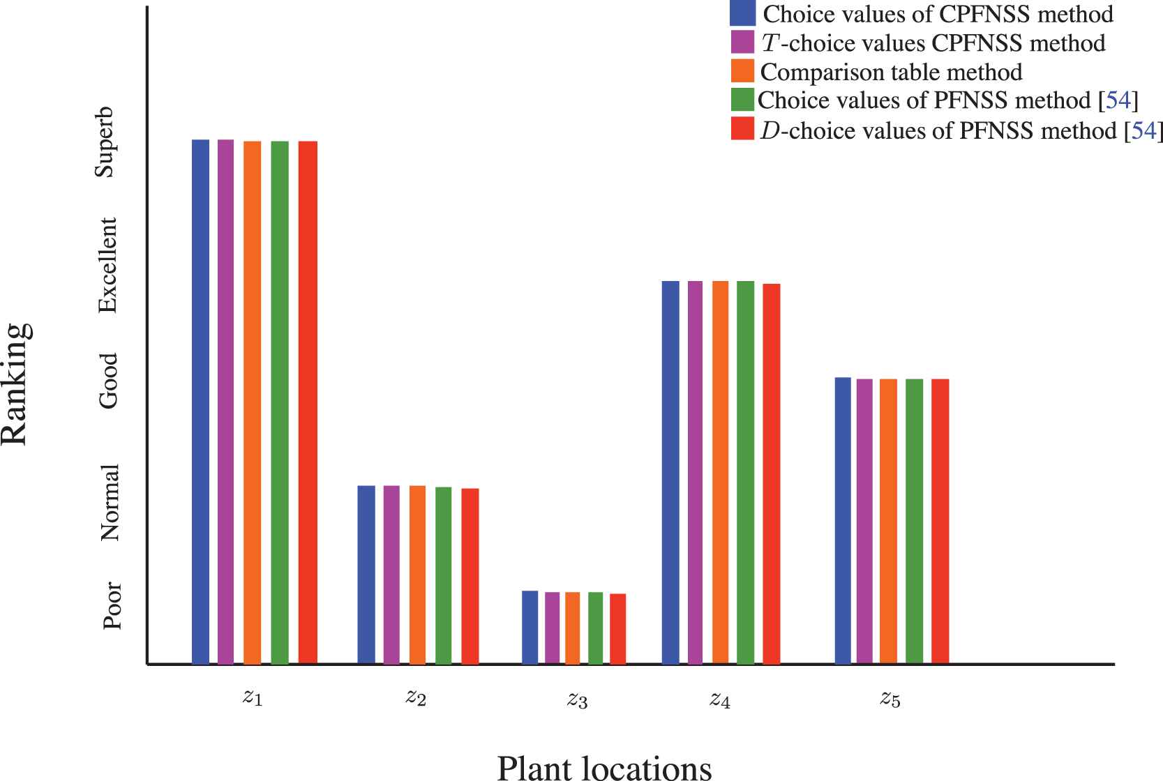
We conduct a comparison with existing MCDM techniques, namely, choice values of PFNSS and D-choice values of PFNSS to demonstrate the proficiency of proposed techniques. The results of compared methods are presented in Table 39.
All the compared and proposed techniques prioritize z₁ as the most profitable location for the start-up of a new manufacturing plant of an enterprise. Also, ranking of plant locations remains the same in all these techniques which depicts the authenticity and validity of our proposed techniques in MADM problems.
The comparison among the results of proposed and existing DM techniques is displayed in Figure 1 by plotting an illustrative bar chart among locations of plant and their order of ranking which demonstrate the reliability and proficiency of the proposed techniques.
Our presented strategies are most generalized and flexible methods as they integrate existing MADM techniques, namely, choice values of PFNSS and D-choice values of PFNSS by capturing both aspects of two-dimensional vague information.
Our proposed techniques have potential to deal with Pythagorean fuzzy N-soft information by taking phase terms equal to zero. Also, they provide the same results as provided by compared techniques. However, compared methods are not capable enough to deal with complex Pythagorean fuzzy N-soft information because of inadequacy of phase terms and they are restricted to capture only one dimensional information. This special trait models our presented techniques superior and stronger than existing DM techniques.
The proposed CPFNSS provides a parameterized mathematical framework for the modeling of fuzziness and vagueness of data. It also has the potential to deal with the obscurity of two-dimensional information, that is, it can capture the uncertainty and periodicity of data at the same time. It is specially designed for the ranking and rating based evaluations of inconsistent and imprecise data.

Methods	Ranking	Best Location
Proposed choice values of CPFNSS method	z1≻z4≻z5≻z2≻z3	z₁
Proposed T-choice values CPFNSS method	z1≻z4≻z5≻z2≻z3	z₁
Proposed comparison table method	z1≻z4≻z5≻z2≻z3	z₁
Choice values of PFNSS method [54]	z1≻z4≻z5≻z2≻z3	z₁
D-choice values of PFNSS method [54]	z1≻z4≻z5≻z2≻z3	z₁

Table 39

Comparative analysis.

7. CONCLUSION

In this research article, a novel theory has been established by the fusion of complex PFS theory with N-soft sets. The powerful and generalized model that arises, abbreviated as CPFNSS, has been introduced to provide a parameterized mathematical tool for the modeling of two-dimensional vague information. It has extrapolated the existing models due to its multinary but discrete evaluations of imprecise parameterized data having complex membership and nonmembership grades. Firstly, we have put forward the formal definition of CPFNSS along with its elementary operations. We have argued that the proposed model has an edge over the existing techniques as it overcomes deficiencies of NSS, PFNSS, CPFS and CIFNSS. Then, we have presented the fundamental Einstein and some algebraic operations of CPFNSVs. Another major contribution of this study is the development of three MCDM approaches for the selection of favorable alternative under CPFNS environment. We have put into practice the presented methodologies on two real life applications to exhibit the significance of our model. Finally, their validity has been demonstrated by comparative analyses with existing MCDM techniques. Admittedly, our presented theory has some limitations because the space of the proposed model is bounded by some constraint conditions. Due to this, the proposed DM methods are restricted to address the MCDM problems within the confined space of the proposed model. Also, the calculations performed by these methods are quite massive and cumbersome. Thus in the future, we are planning to extend our research to the more generalized mathematical theories covering a broader range of space and reduce the lengthy calculations of these DMtechniques by computer programing. We also intend to develop more MCDM strategies, including TOPSIS method, VIKOR method and ELECTRE I method under such a rich and flexible environment of CPFNSS.

CONFLICTS OF INTEREST

The authors declare no conflict of interest.

AUTHORS' CONTRIBUTIONS

Muhammad Akram proposed the methodology; Faiza Wasim investigated the results; Ahmad N. Al-Kenani reviewed the results. All authors read and approved the final manuscript.

ACKNOWLEDGMENTS

This project was funded by the Deanship of Scientific Research (DSR), King Abdulaziz University, Jeddah, under grant No. (RG-24-130-38). The authors, therefore, gratefully acknowledge DSR technical and financial support.

REFERENCES

1.M. Akram, A. Adeel, and J.C.R. Alcantud, Group decision-making methods based on hesitant N-soft sets, Expert Syst. Appl., Vol. 115, 2019, pp. 95-105.

2.M. Akram, A. Adeel, and J.C.R. Alcantud, Fuzzy N-soft sets: a novel model with applications, J. Intell. Fuzzy Syst., Vol. 35, 2018, pp. 4757-4771.

3.M. Akram, A. Adeel, and J.C.R. Alcantud, Hesitant fuzzy N-soft sets: a new model with applications in decision-making, J. Intell. Fuzzy Syst., Vol. 36, 2019, pp. 6113-6127.

4.M. Akram, G. Ali, and J.C.R. Alcantud, New decision-making hybrid model: intuitionistic fuzzy N-soft rough sets, Soft Comput., Vol. 23, 2019, pp. 9853-9868.

5.M. Akram, H. Garg, and K. Zahid, Extensions of ELECTRE-I and TOPSIS methods for group decision-making under complex Pythagorean fuzzy environment, Iranian J. Fuzzy Syst., Vol. 17, 2020, pp. 147-164.

6.M. Akram, A. Luqman, and J.C.R. Alcantud, Risk evaluation in failure modes and effects analysis: hybrid TOPSIS and ELECTRE I solutions with Pythagorean fuzzy information, Neural Comput. Appl., 2021.

7.M. Akram, A. Adeel, A.N. Al-Kenani, and J.C.R. Alcantud, Hesitant fuzzyN-soft ELECTRE-II model: a new framework for decision-making, Neural Comput. Appl., 2020.

8.M. Akram and S. Naz, A novel decision-making approach under complex Pythagorean fuzzy environment, Math. Comput. Appl., Vol. 24, 2019, pp. 73.

9.J.C.R. Alcantud, F. Feng, and R.R. Yager, An N-soft set approach to rough sets, IEEE Trans. Fuzzy Syst., Vol. 28, 2020, pp. 2996-3007.

10.A.S. Alkouri and A.R. Salleh, Complex intuitionistic fuzzy sets, AIP Conf. Proc., Vol. 1482, 2012, pp. 464-470.

11.K.T. Atanassov, Intuitionistic fuzzy sets, Fuzzy Sets Syst., Vol. 20, 1986, pp. 87-96.

12.Z.S. Chen, X.L. Liu, R.M. Rodríguez, X.J. Wang, K.S. Chin, K.L. Tsui, and L. Martínez, Identifying and prioritizing factors affecting in-cabin passenger comfort on high-speed rail in China: afuzzy-based linguistic approach, Appl. Soft Comput., Vol. 95, 2020, pp. 106558.

13.Z.S. Chen, Y. Yang, X.J. Wang, K.S. Chin, and K.L. Tsui, Fostering linguistic decision-making under uncertainty: a proportional interval type-2 hesitant fuzzy TOPSIS approach based on Hamacher aggregation operators and andness optimization models, Inf. Sci., Vol. 500, 2019, pp. 229-258.

14.Z.S. Chen, C. Yu, K.S. Chin, and L. Martínez, An enhanced ordered weighted averaging operators generation algorithm with applications for multi-criteria decision making, Appl. Math. Model., Vol. 71, 2019, pp. 467-490.

15.F. Fatimah and J.C.R. Alcantud, The multi-fuzzy N-soft set and its applications to decision-making, Neural Comput. Appl., 2021.

16.F. Fatimah, D. Rosadi, R.B.F. Hakim, and J.C.R. Alcantud, N-soft sets and their decision making algorithms, Soft Comput., Vol. 22, 2018, pp. 3829-3842.

17.F. Feng, Soft rough sets applied to multi criteria group decision making, Ann. Fuzzy Math. Inform., Vol. 2, 2011, pp. 69-80.

18.F. Feng, M. Akram, B. Davvaz, and V.L. Fotea, Attribute analysis of information systems based on elementary soft implications, Knowl.-Based Syst., Vol. 70, 2014, pp. 281-292.

19.F. Feng, X. Liu, V. Leoreanu-Fotea, and Y.B. Jun, Soft sets and soft rough sets, Inf. Sci., Vol. 181, 2011, pp. 1125-1137.

20.H. Garg, Linguistic Pythagorean fuzzy sets and its applications in multi attribute decision making process, Int. J. Intell. Syst., Vol. 33, 2018, pp. 1234-1263.

21.H. Garg, Hesitant Pythagorean fuzzy sets and their aggregation operators in multiple-attribute decision-making, Int. J. Uncertain. Quant., Vol. 8, 2018, pp. 267-289.

22.H. Garg, A novel correlation coeﬃcients between Pythagorean fuzzy sets and its applications to decision-making processes, Int. J. Intell. Syst., Vol. 31, 2016, pp. 1234-1253.

23.C. Huang, M. Lin, and Z. Xu, Pythagorean fuzzy MULTIMOORA method based on distance measure and score function: its application in multicriteria decision making process, Knowl. Inf. Syst., Vol. 62, 2020, pp. 4373-4406.

24.T. Kumar and R.K. Bajaj, On complex intuitionistic fuzzy soft sets with distance measures and entropies, J. Math., Vol. 2014, 2014, pp. 1-12.

25.M. Lin, Z. Chen, Z. Xu, X. Gou, and F. Herrera, Score function based on concentration degree for probabilistic linguistic term sets: an application to TOPSIS and VIKOR, Inf. Sci., Vol. 551, 2021, pp. 270-290.

26.M. Lin, C. Huang, R. Chen, H. Fujita, and X. Wang, Directional correlation coeﬃcient measures for Pythagorean fuzzy sets: their applications to medical diagnosis and cluster analysis, Complex Intell. Syst., Vol. 7, 2021, pp. 1025-1043.

27.M. Lin, C. Huang, and Z. Xu, TOPSIS method based on correlation coeﬃcient and entropy measure for linguistic Pythagorean fuzzy sets and its application to multiple attribute decision making, Complexity, Vol. 2019, 2019, pp. 1-16.

28.M. Lin, C. Huang, Z. Xu, and R. Chen, Evaluating IoT platforms using integrated probabilistic linguistic MCDM method, IEEE Internet Things J., Vol. 7, 2020, pp. 11195-11208.

29.M. Lin, X. Li, and L. Chen, Linguistic q-rung orthopair fuzzy sets and their interactional partitioned Hero-nian mean aggregation operators, Int. J. Intell. Syst., Vol. 35, 2020, pp. 217-249.

30.M. Lin, W. Xu, Z. Lin, and R. Chen, Determine OWA operator weights using kernel density estimation, Econ. Res.-Ekon. Istraz., Vol. 33, 2020, pp. 1441-1464.

31.Y. Liu, J.C.R. Alcantud, R.M. Rodríguez, K. Qin, and L. Martínez, Intertemporal hesitant fuzzy soft sets: application to group decision making, Int. J. Fuzzy Syst., Vol. 22, 2020, pp. 619-635.

32.Y. Liu, R.M. Rodríguez, J.C.R. Alcantud, K. Qin, and L. Martínez, Hesitant linguistic expression soft sets: application to group decision making, Comput. Ind. Eng., Vol. 136, 2019, pp. 575-590.

33.D. Molodtsov, Soft set theory-first results, Comput. Math. Appl., Vol. 37, 1999, pp. 19-31.

34.Z. Pawlak, Rough sets, Int. J. Comput. Inf. Sci., Vol. 11, 1982, pp. 341-356.

35.X. Peng, Y. Yang, and J. Song, Pythagorean fuzzy soft set and its application, Comput. Eng., Vol. 41, 2015, pp. 224-229.

36.D. Ramot, M. Friedman, G. Langholz, and A. Kandel, Complex fuzzy logic, IEEE Trans. Fuzzy Syst., Vol. 11, 2003, pp. 450-461.

37.D. Ramot, R. Milo, M. Friedman, and A. Kandel, Complex fuzzy sets, IEEE Trans. Fuzzy Syst., Vol. 10, 2002, pp. 171-186.

38.D. Rani and H. Garg, Complex intuitionistic fuzzy power aggregation operators and their applications in multicriteria decision-making, Expert Syst., Vol. 35, 2018, pp. e12325.

39.R.M. Rodríguez, A. Labella, B. Dutta, and L. Martínez, Comprehensive minimum cost models for large scale group decision making with consistent fuzzy preference relations, Knowl.-Based Syst., Vol. 215, 2021, pp. 106780.

40.R.M. Rodríguez, A. Labella, G.D. Tre, and L. Martínez, A large scale consensus reaching process managing group hesitation, Knowl.-Based Syst., Vol. 159, 2018, pp. 86-97.

41.B. Schweizer and A. Sklar, Probabilistic Metric Spaces, North-Holland, New York, NY, USA, 1983.

42.P. Thirunavukarasu, R. Suresh, and V. Ashokkumar, Theory of complex fuzzy soft set and its applications, Int. J. Innov. Res. Sci. Technol., Vol. 3, 2017, pp. 13-18.

43.K. Ullah, T. Mahmood, Z. Ali, and N. Jan, On some distance measures of complex Pythagorean fuzzy sets and their applications in pattern recognition, Complex Intell. Syst., Vol. 6, 2020, pp. 15-27.

44.J.C. Wang and T.Y. Chen, A novel Pythagorean fuzzy LINMAP-based compromising approach for multiple criteria group decision-making with preference over alternatives, Int. J. Comput. Intell. Syst., Vol. 13, 2020, pp. 444-463.

45.L. Wang and H. Garg, Algorithm for multiple attribute decision-making with interactive archimedean norm operations under Pythagorean fuzzy uncertainty, Int. J. Comput. Intell. Syst., Vol. 14, 2021, pp. 503-527.

46.L. Wang and N. Li, Pythagorean fuzzy interaction power Bonferroni mean aggregation operators in multiple attribute decision making, Int. J. Intell. Syst., Vol. 35, 2020, pp. 150-183.

47.G. Wei and M. Lu, Pythagorean fuzzy power aggregation operators in multiple attribute decision making, Int. J. Intell. Syst., Vol. 33, 2018, pp. 169-186.

48.R.R. Yager and A.M. Abbasov, Pythagorean membership grades, complex numbers and decision making, Int. J. Intell. Syst., Vol. 28, 2013, pp. 436-452.

49.R.R. Yager, Pythagorean membership grades in multicriteria decision making, IEEE Trans. Fuzzy Syst., Vol. 22, 2013, pp. 958-965.

50.R.R. Yager, Pythagorean fuzzy subsets, in 2013 Joint IFSA World Congress and NAFIPS Annual Meeting (IFSA/NAFIPS) (Edmonton, Canada), 2013, pp. 57-61.

51.R.R. Yager, On ordered weighted averaging aggregation operators in multicriteria decision making, IEEE Trans. Syst. Man Cybern., Vol. 18, 1988, pp. 183-190.

52.Y. Yang, Z.S. Chen, R.M. Rodriguez, W. Pedrycz, and K.S. Chin, Novel fusion strategies for continuous interval-valued q-rung orthopair fuzzy information: a case study in quality assessment of SmartWatch appearance design, Int. J. Mach. Learn. Cybern., 2021.

53.L.A. Zadeh, Fuzzy sets, Inf. Control, Vol. 8, 1965, pp. 338-353.

54.H. Zhang, D.J. Hua, and C. Yan, Multi-attribute group decision-making methods based on Pythagorean fuzzy N-soft sets, IEEE Access, Vol. 8, 2020, pp. 62298-62309.

55.X. Zhang and Z. Xu, Extension of TOPSIS to multiple criteria decision making with pythagorean fuzzy sets, Int. J. Intell. Syst., Vol. 29, 2014, pp. 1061-1078.

56.F. Zhou and T.Y. Chen, A novel distance measure for Pythagorean fuzzy sets and its applications to the technique for order preference by similarity to ideal solutions, Int. J. Comput. Intell. Syst., Vol. 12, 2019, pp. 955-969.

<Previous Article In Issue

Download article (PDF)

Next Article In Issue>

Journal: International Journal of Computational Intelligence Systems
Volume-Issue: 14 - 1
Pages: 1263 - 1291
Publication Date: 2021/04/12
ISSN (Online): 1875-6883
ISSN (Print): 1875-6891
DOI: 10.2991/ijcis.d.210331.002 How to use a DOI?
Open Access: This is an open access article distributed under the CC BY-NC 4.0 license (http://creativecommons.org/licenses/by-nc/4.0/).

Cite this article

ris enw bib

TY  - JOUR
AU  - Muhammad Akram
AU  - Faiza Wasim
AU  - Ahmad N. Al-Kenani
PY  - 2021
DA  - 2021/04/12
TI  - A Hybrid Decision-Making Approach Under Complex Pythagorean Fuzzy N-Soft Sets
JO  - International Journal of Computational Intelligence Systems
SP  - 1263
EP  - 1291
VL  - 14
IS  - 1
SN  - 1875-6883
UR  - https://doi.org/10.2991/ijcis.d.210331.002
DO  - 10.2991/ijcis.d.210331.002
ID  - Akram2021
ER  -

download .riscopy to clipboard