
Certain Properties of Single-Valued Neutrosophic Graph With Application in Food and Agriculture Organization
 , Hossein Rashmanlou6, Farshid Mofidnakhaei7,
 - DOI
- 10.2991/ijcis.d.210413.001How to use a DOI?
- Keywords
- Single-valued neutrosophic graph; maximal product; rejection; symmetric difference; residue product
- Abstract
Fuzzy graph models are present everywhere from natural to artificial structures, embodying the dynamic processes in physical, biological, and social systems. As real-life problems are often uncertain on account of inconsistent and indeterminate information, it seems very demanding for an expert to model those problems using a fuzzy graph. To deal with the uncertainty associated with the inconsistent and indeterminate information of any real-world problems, a neutrosophic graph can be applied, where fuzzy graphs may not bear any fruitful results. The past definitions limitations in fuzzy graphs have directed us to present new definitions in single-valued neutrosophic graph (SVNG). A SVNG has several applications in the fields of physics, bio and connectivity of socialism. It has been an advantageous scope in the recent times for providing such information which is incomplete or uncertain accounting in real problems that gives the direction to describe the relationship between nodes. Operations are conveniently used in many combinatorial applications. In various situations, they present a suitable construction means; therefore, the current study, seeks to present and explore the key features of new operations, including: rejection, maximal product, symmetric difference, and residue product of SVNG. We have discuss the concept of maximal product on two strong-(SVNGS) and maximal product of connected-SVNG with examples. This research article presents the notions of degree of a vertex and total degree of a vertex in SVNG. Moreover, this study summarizes the specific conditions needed for obtaining vertices degrees in SVNG under the operations of maximal product, symmetric difference, residue product, and rejection. In addition, an application was illustrated in the food and agriculture organization with an algorithm to emphasize the contributions of this research article in practical applications.
- Copyright
- © 2021 The Authors. Published by Atlantis Press B.V.
- Open Access
- This is an open access article distributed under the CC BY-NC 4.0 license (http://creativecommons.org/licenses/by-nc/4.0/).
1. INTRODUCTION
Graph theory is an exceptionally advantageous device in tackling combinatorial issues in different regions including calculation, variable-based math, number hypothesis, geography, and social frameworks. A graph is chiefly a model of relations, and it is applied to speak to the genuine issues including connections between objects. The vertices and edges of the graph are utilized to connote the articles and the relations between objects, individually. In numerous improvement issues, the current data is vague or loose for different reasons, for example, the loss of data, the absence of proof, flawed measurable information, and inadequate data. By and large, the vulnerability, in actuality, issues may show up in the data that characterizes the issue. Fuzzy chart models are important numerical apparatuses for treating the combinatorial issues of different areas enveloping exploration, streamlining, variable-based math, figuring, ecological science, and geography. Fuzzy graphical models are observably more helpful than graphical models due to the common presence of unclearness and equivocalness. Initially, fuzzy set hypothesis is needed to manage numerous perplexing issues including inadequate data. Zadeh [32], firstly exemplified the idea of the set known as the fuzzy set. He described the fuzzy set characterized by true membership function value ranging from closed interval [0, 1]. Fuzzy set theory serves as a very powerful mathematical tool for solving approximate reasoning related problems. These notions effectively illustrate complex phenomena, which are not precisely described by classical mathematics.
The fuzzy graphs idea and concept are discussed by Smarandache and Rosenfeld [27]. The fuzzy graphs application has been extended in few years and it has a scope from 19th century [4,5,10,11,15,16]. It is not necessarily true membership degree of 1, also, the nonmembership degree and indeterminacy occur. Nonmembership degree is presented by Atanassove [3] in an intuitionistic fuzzy set. Shao et al. [31] labeled new concepts of bondage number in intuitionistic fuzzy graph. Rashmanlou et al. [20–26] introduced new concepts in bipolar fuzzy graph and interval-valued fuzzy graphs. Krishna et al. [13,14] analyzed the concept of vague set and vague graph. Devi et al. [8] investigated new ways in intuitionistic fuzzy labeling graph. Pythagorean fuzzy set also known as IF-set of type-2 [1] is the extension of intuitionistic fuzzy set (IF-set). Parvathi and Karunambigai [19] studied about Intuitionistic fuzzy graphs. After while, Smarandache [31] included the indeterminacy concept in a neutrosophic set. Neutrosophy is the kind of philosophy which analyzes the nature and scope of neutralities. Neutrosophic set is the speculation of fuzzy set and furthermore neutrosophic rationale is the expansion of fuzzy rationale. Smarandache gives the possibility of a neutrosophic set due to introducing the vulnerability in the issues of different fields like clinical science and financial aspects and so forth. He portrayed significant classifications [29] of neutrosophic diagrams from which two classifications are relied upon the strict indeterminacy and other two classes depended [7] on its (t, i, f) parts. Malik and Hassan [12] presented the classification of bipolar single-valued neutrosophic graph (SVNG) classification. Later Malik and Naz et al. [17] described new operations on SVNG. Naz et al. [17] discussed operations on single-valued neutrosophic graphs with application. Malik et al. [18] also investigated some properties of bipolar SVNG. Product operations have applications in different branches, such as coding theory, network designs, chemical graph theory, and others. Many scholars discussed product operations on various generalized FGs. Mordeson and Peng [16] defined some of these product operations on FGs and some new fuzzy models are discussed in [33–38].
In this research, some new properties, including maximal product, symmetric difference, residue product, and rejection of SVNG are presented. Also, the examples of these operations are discussed. We found the degree and the total degree of SVNG. Finally, an application was illustrated in the food and agriculture organization with an algorithm to highlight the contributions of this research article in practical applications.
2. PRELIMINARIES
In this section, the key preliminary notions and definitions that are used in this current research study will be introduced.
Definition 1.
[9] A graph G = (V, E) is an ordered pair of set of vertices and set of edges.
Definition 2.
[30] Suppose that X is a space of points with generic element in X denoted by x. Then, the neutrosophic set M (NS-M) is defined as M = < x : TM(x), IM(x), FM(x) >, x ∈ X which obey 0 ⩽ {TM(x) + IM(x) + FM(x)} ⩽ 3. TM : V → [0, 1], IM: V → [0, 1], and FM : V → [0, 1] represents the degree of true membership function, degree of indeterminacy membership function, and degree of false membership function of the element x ∈ X, respectively.
Definition 3.
[27] A SVNG G = (M, N) with underlying set of V is defined to be a pair of G = (V, E) which is defined as (i) TM : V → [0, 1], FM : V [0, 1] and IM : V → [0, 1] represents the degree of true membership function, degree of false membership function, and degree of indeterminacy membership function of the element m ∈ V, respectively, where 0 ⩽ TM(m) +IM(m)+FM(m) ⩽ 3, ∀ m ∈ V.
(ii) The function TN : E → [0, 1], IN : E → [0, 1] and FN : E → [0, 1] are defined by
It is free of any restriction so 0 ⩽ TN(mn)+IN(mn)+FN(mn) ⩽ 3.
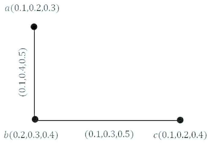
Example 1.
Consider the Figure 1 such that V = {a, b, c}, E = {ab, bc, ca},
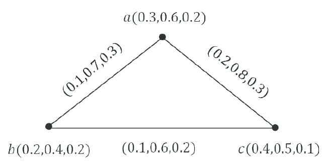
SVNG(G).
By routine computations, it is easy to show that G is a SVNG.
Definition 4.
A SVNG G is said to be strong if TN(mn) = min(TM(m), TM(n)), IN(mn) = max(IM(m), IM(n)) and FN(mn) = max(FM(m), FM(n)), for all mn in V.
Definition 5.
A SVNG G is said to be complete if TN(mn) = min(TM(m), TM(n)), IN(mn) = max(IM(m), IM(n)) and FN(mn) = max(FM(m), FM(n)), for all m, n in E.
Definition 6.
A SVNG G is said to be connected if
3. OPERATIONS ON SVNGs
In this section, we define four new kinds of operations on (SVNGs) including maximal product, residue product, rejection, and symmetric difference. We show that maximal product, residue product, and rejection of two (SVNGs) are a SVNG.
Definition 7.
The maximal product G1 ∗ G2 = (M1 ∗ M2, N1 ∗ N2) of two (SVNGs) G1 = (M1, N1) and G2 = (M2, N2) is defined as
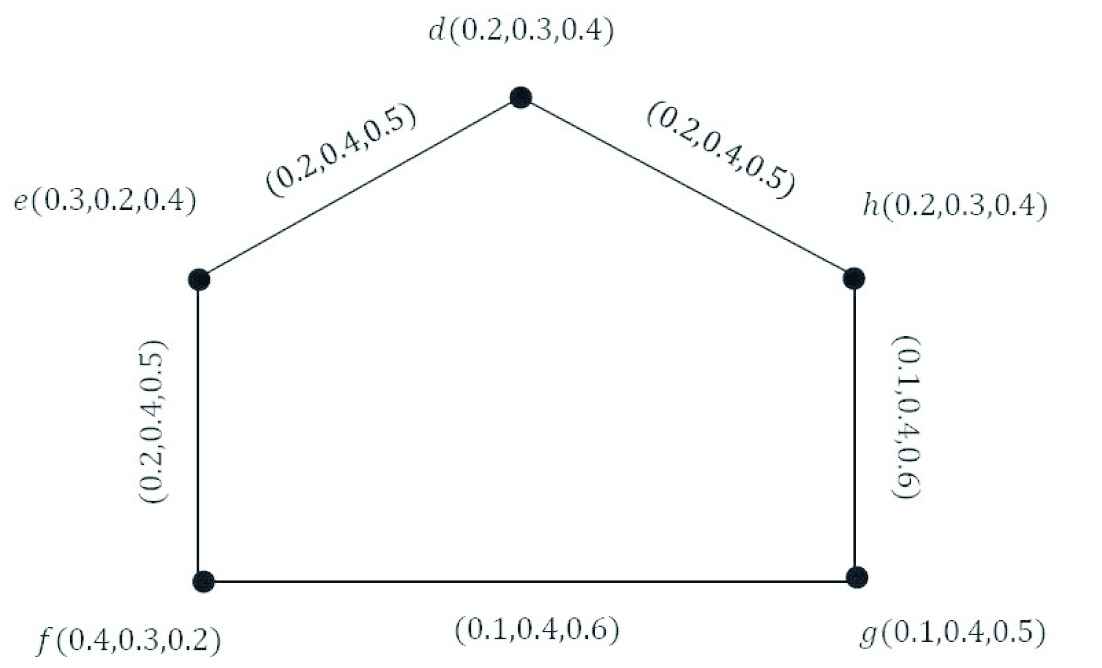
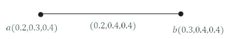
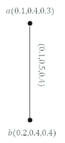
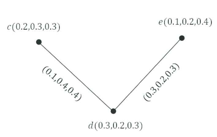
Example 2.
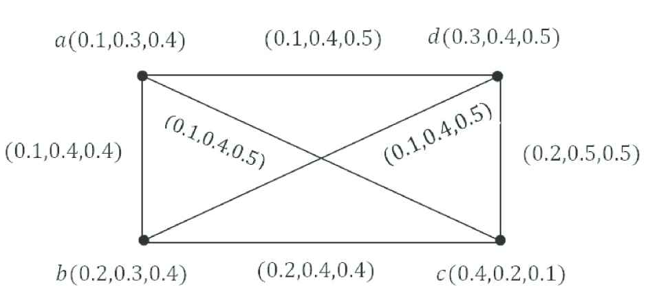
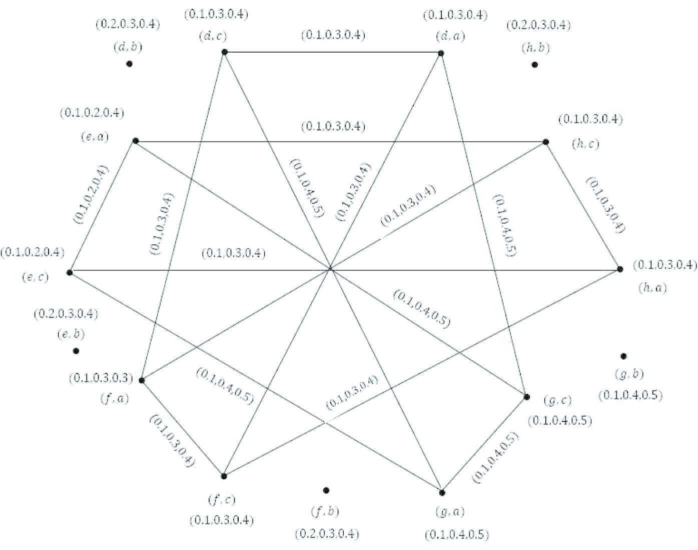
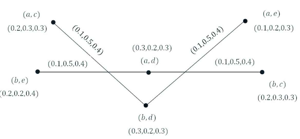
Consider two (SVNGs) G1 = (M1, N1) and G2 = (M2, N2), as shown in Figures 2 and 3. Their maximal product G1 ∗ G2 is shown in Figure 4.
G1. G2. G1 * G2.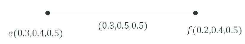
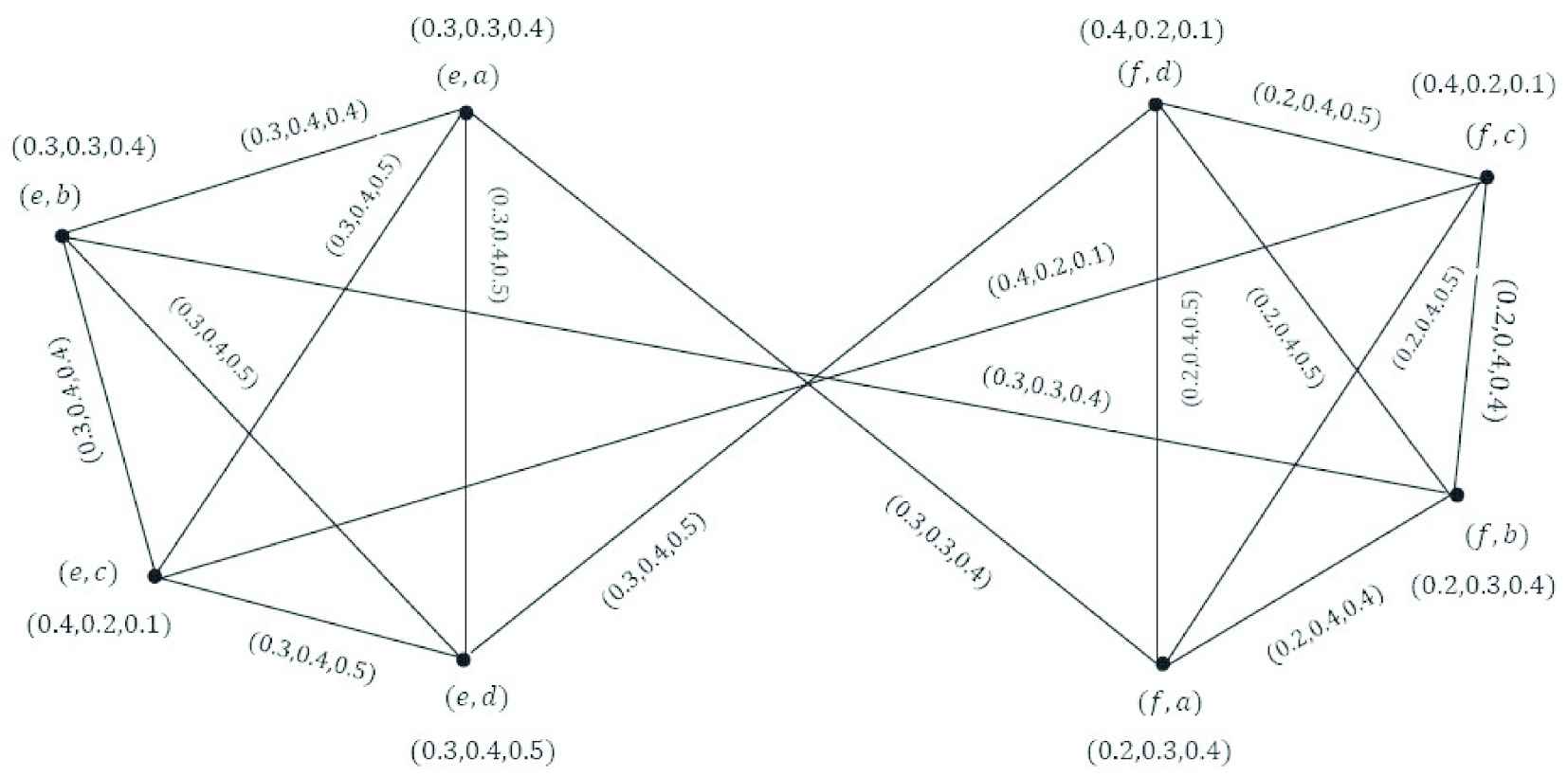
For vertex (e, a), we find membership value, indeterminacy and nonmembership value as follows:
Similarly, we can find membership, indeterminacy, and nonmembership value for all remaining vertices and edges.
Proposition 1.
The maximal product of two (SVNGs) G1and G2, is a SVNG.
Proof.
Let G1 = (M1, N1) and G2 = (M2, N2) be two (SVNGs) on crisp graphs G1 = (V1, E1) and G2 = (V2, E2), respectively and ((m1, m2)(n1, n2)) ∈ E1 × E. Then, by Definition 7, we have two cases:
If m1 = n1 = m
If m2 = n2 = z
Therefore, G1 ∗ G2 is a SVNG.
Theorem 2.
The maximal product of two strong-(SVNGS) G1and G2, is a strong-SVNG.
Proof.
Let G1 = (M1, N1) and G2 = (M2, N2) be two strong-(SVNGS) on crisp graphs G1 = (V1, E1) and G2 = (V2, E2), respectively and ((m1, m2)(n1, n2)) ∈ E1 × E2. Then by Proposition 1, G1 ∗ G2 is a SVNG. Now we have two cases:
If m1 = n1 = m
If m2 = n2 = z
Therefore, G1 * G2 is a strong-SVNG.
Example 3.
Consider the strong-(SVNGS) G1 and G2 as in Figure 5.
Single-valued neutrosophic graphs.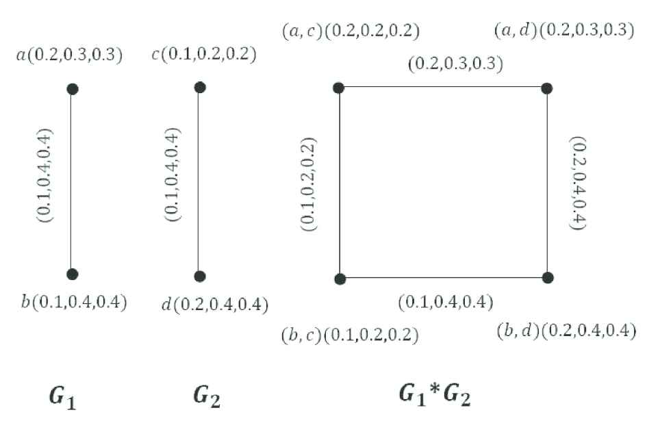
It is easy to see that G1 * G2 is a strong-SVNG, too.
Remark 1.
If the maximal product of two (SVNGs) G1 = (M1, N1) and G2 = (M2, N2) is strong, then G1 = (M1, N1) and G2 = (M2, N2) need not to be strong, in general.
Example 4.
Consider the (SVNGs) G1 and G2 as in Figures 6 and 7. We can see that the maximal product of two (SVNGs) G1 and G2, that is G1 * G2 in Figure 8.
G1. G2. G1 * G2.
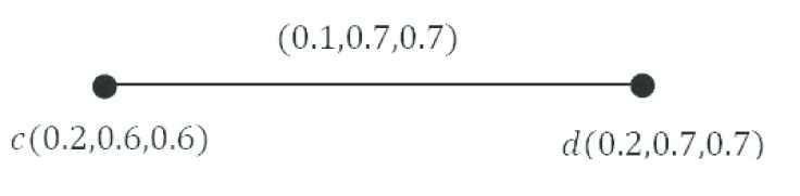
Then G1 and G1 * G2 are strong-(SVNGS), but G2 is not strong. Since
Theorem 3.
The maximal product of two connected-(SVNGs) is a connected-SVNG.
Proof.
Let G1 = (M1, N1) and G2 = (M2, N2) be two connected-(SVNGs) on crisp graphs G1 = (V1, E1) and G2 = (V2, E2), respectively, where V1 = {m1, m2, ⋯ mk} and V2 = {n1, n2, ⋯ ns}. Then
Hence, there exists at least one edge between any pair of the above “k” subgraphs. Thus we have
Remark 2.
The maximal product of two complete-(SVNGs) is not a complete-SVNG, in general. Because we do not include the case (m1, m2) ∈ E1 and (n1, n2) ∈ E2 in the definition of the maximal prod-uct of two (SVNGs).
Remark 3.
The maximal product of two complete-(SVNGS) is a strong-SVNG.
Example 5.
Consider the complete-(SVNGs) G1 and G2 as in Figure 5. A simple calculation concludes that G1*G2 is a strong-SVNG.
Definition 8.
Let G1 = (M1, N1) and G2 = (M2, N2) be two (SVNGs). ∀(m1, m2) ∈ V1×V2:
Theorem 4.
Let G1 = (M1, N1) and G2 = (M2, N2) are two (SVNGs). If
Proof.
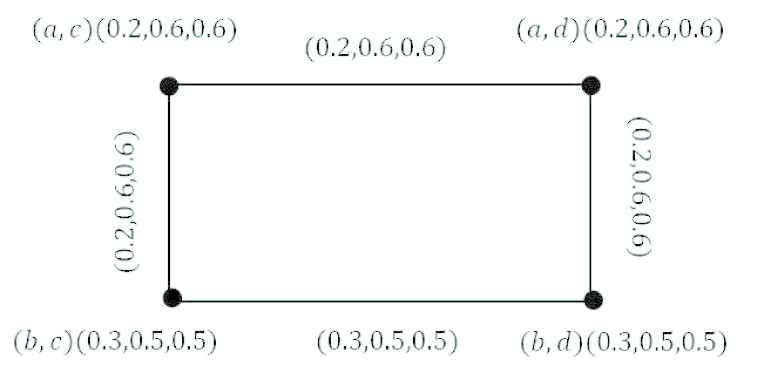
Example 6.
Consider the (SVNGs) G1,G2, and G1*G2 as in Figure 9. Since
Single-valued neutrosophic graphs.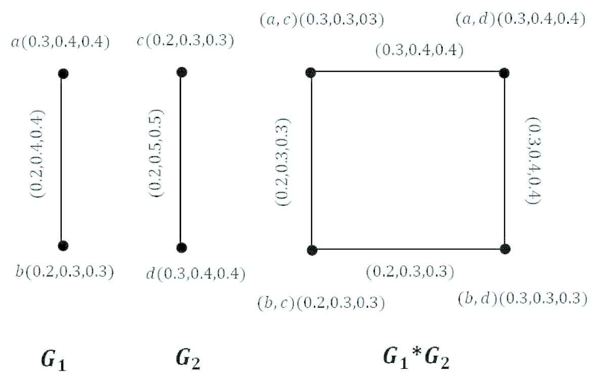
By direct calculations:
It is clear from the above calculations that the degrees of vertices calculated by using the formula of the above theorem and by directed method are the same.
Definition 9.
Let G1 = (M1, N1) and G2 = (M2, N2) be two (SVNGs). For any vertex (m1, m2) ∈ V1 × V2 we have
Theorem 5.
Let G1 = (M1, N1) and G2 = (M2, N2) be two (SVNGs). If
Proof.
Example 7.
Consider the (SVNGs) G1, G1, and G1∗G2 as in Figures 2–4. We find the total degree of vertices in maximal product. Hence, we choose vertex (e,a).
In the same way we can find the total degree for all remaining vertices.
Definition 10.
The rejection G1|G2 = (M1|M2, N1|N2) of two (SVNGs) G1 = (M1, N1) and G2 = (M2, N2) is defined as
Example 8.
Consider the (SVNGs) G1 and G2 as in Figures 10 and 11. We can see that the rejection of two (SVNGs) G1 and G2, that is G1|G2 in Figure 12.
G1.
G2.
G1|G2.
For vertex (e, a), we find true membership value, indeterminacy, and false membership value as follows:
Similarly, we can find both membership and non-membership value for all remaining vertices and edges.
Proposition 6.
The rejection of two (SVNGs) G1and G2, is a SVNG.
Proof.
Let G1 = (M1, N1) and G2 = (M2, N2) be two (SVNGs) on crisp graphs G1 = (V1, E1) and G2 = (V2, E2), respectively and (m1, m2)(n1, n2)) ∈ E1 × E2. Then by Definition 10, we have
If m1 = n1, m2n2 ∉ E2
If m2 = n2, m1n1 ∉ E1
If m1n1 ∉ E1and m2n2 ∉ E2
Therefore, G1|G2 = (M1|M2, N1|N2) is a SVNG.
Remark 4.
The rejection of two complete (SVNGs) G1 = (M1, N1) and G2 = (M2, N2) is a complete-SVNG.
Definition 11.
Let G1 = (M1, N1) and G2 = (M2, N2) be two (SVNGs). For any vertex (m1, m2) ∈ V1×V2 we have
Definition 12.
Let G1 = (M1, N1) and G2 = (M2, Y2) be two (SVNGs). ∀(m1, m2) ∈ V1×V2
Example 9.
In this example we find the degree and the total degree of vertex (d, a) in Example 8.
Hence,
In addition, by definition of total vertex degree in rejection,
So,
Similarly, we can find the degree and the total degree of all vertices in G1|G2.
Definition 13.
The symmetric difference G1 ⊕ G2 = (M1 ⊕ M2, N1 ⊕ N2) of two (SVNGs) G1 = (M1, N1) and G2 = (M2, N2) is defined as
(TN1 ⊕ TN2)((m1, m2)(n1, n2)) = min{TM1(m1), TM1(n1),
TN2(m2n2)} forall m1n1 ∉ E1and m2n2 ∈ E2
or
= min{TM2(m2), TM2(n2), TN1(m1n1)}
forall m1n1∈ E1and m2n2 ∉ E2,
(IN1 ⊕ IN2)((m1, m2)(n1, n2)) = max{IM1(m1), IM1(n1),
IN2(m2n2)} forall m1n1 ∉ E1and m2n2∈ E2
or
= max{IM2(m2), IM2(n2), IN1(m1n1)}
forall m1n1∈ E1and m2n2∉ E2,
or
Example 10.
Consider the (SVNGs) G1 and G2 as in Figures 13 and 14. We can see the symmetric difference of two (SVNGs) G1 and G2, that is G1 ⊕ G2 in Figure 15.
G1.

G2.

G1 ⊕ G2.
For vertex (a, f), we find the true membership value, indeterminacy, and the false membership value as follows:
For edge (a, d) (a, e), we calculate the true membership value, indeterminacy, and the false membership value.
Now, for edge (a, d)(b, d) we have
Finally, for edge (a, c)(b, f) we can find the true membership value, indeterminacy, and the false membership value as follows:
Proposition 7.
The symmetric difference of two (SVNGs) G1and G2, is a SVNG.
Proof.
Let G1 = (M1, N1) and G2 = (M2, N2) be two (SVNGs) on crisp graphs G1 = (V1, E1) and G2 = (V2, E2), respectively and ((m1, m2)(n1, n2)) ∈ E1 ×E2. Then by Definition 3.21 we have
If m1 = n1 = m
If m2 = n2 = z
If m1n1 ∈ E1and m2n2 ∉ E2
If m1n1 ∈ E1and m2n2 ∉ E2
Hence, G1 ⊕ G2 is a SVNG.
Remark 5.
The symmetric difference of two connected-(SVNGs) G1 = (M1, N1) and G2 = (M2, N2) is connected. Because we include the case (m1, m2) ∈ E1 and (n1, n2) ∈ E2 in the definition of the symmetric difference of two (SVNGs).
Definition 14.
Let G1 = (M1, N1) and G2 = (M2, N2) be two (SVNGs). For any vertex (m1, m2) ∈ V1×V2 we have
Theorem 8.
Let G1 = (M1, N1) and G2 = (M2, Y2) be two (SVNGs). If
Proof.
We conclude that
Example 11.
In Figure 16,

Symmetric difference.
Hence,
It is obvious from the above calculations that the degrees of vertices calculated by using the formula of the above theorem and by direct method are the same.
Definition 15.
Let G1 = (M1, N1) and G2 = (M2, N2) be two (SVNGs). For any vertex (m1, m2) ∈ V1 × V2 we have
Theorem 9.
Let G1 = (M1, N1) and G2 = (M2, Y2) be two (SVNGs).
If
If
If
Proof.
∀(m1, m2) ∈ V1×V2 we have
Example 12.
In this example, we calculate the total degree of vertices in Example 10.
Similarly,
It is clear from the above calculations that total degrees of vertices calculated by using the formula of the above theorem and by direct method are same.
Definition 16.
The residue product
Example 13.
Consider the (SVNGs) G1 and G2 as in Figures 17 and 18. We can see the residue product of two (SVNGs) G1 and G2, that is G1 • G2 in Figure 19.
G1.
G2.
G1 ⊕ G2.
For vertex (b, e), we find the true membership value, indeterminacy, and the false membership value as follows:
For edge (a, c) (b, d), we calculate the true membership value, indeterminacy, and the false membership value as follows:
Similarly, we can find the true membership value, indeterminacy, and the false membership value for all remaining vertices and edges.
Proposition 10.
The residue product of two (SVNGs) G1and G2, is a SVNG.
Proof.
Let G1 = (M1, N1) and G2 = (M2, N2) be two (SVNGs) on crisp graphs G1 = (V1, E1) and G2 = (V2, E2), respectively and ((m1, m2)(n1, n2)) ∈ E1 × E2. If m1n1 ∈ E1and m2 ≠ n2 then we have
Definition 17.
Let G1 = (M1, N1) and G2 = (M2, N2) be two (SVNGs). For any vertex (m1, m2) ∈ V1 × V2 we have
Definition 18.
Let G1 = (M1, N1) and G2 = (M2, N2) be two (SVNGs). For any vertex(m1, m2) ∈ V1 × V2 we have
Example 14.
In this example we find the degree and the total degree of vertex (b, e) in Example 13.
| R1 | b1 | b2 | b3 | b4 | b5 |
|---|---|---|---|---|---|
| b1 | <0.5, 0.5, 0.5> | <0.2, 0.8, 0.1> | <0.1, 0.6, 0.2> | <0.2, 0.3, 0.6> | <0.1, 0.2, 0.4> |
| b2 | <0.1, 0.2, 0.2> | <0.5, 0.5, 0.5> | <0.2, 0.4, 0.7> | <0.1, 0.4, 0.2> | <0.9, 0.3, 0.4> |
| b3 | <0.1, 0.4, 0.2> | <0.7, 0.6, 0.2> | <0.5, 0.5, 0.5> | <0.6, 0.3, 0.2> | <0.4, 0.2, 0.6> |
| b4 | <0.6, 0.7, 0.1> | <0.2, 0.6, 0.1> | <0.2, 0.7, 0.6> | <0.5; 0.5; 0.5> | <0.3; 0.2; 0.7> |
| b5 | <0.4, 0.8, 0.1> | <0.4, 0.7, 0.9> | <0.6, 0.8, 0.4> | <0.7, 0.8, 0.3> | <0.5; 0.5; 0.5> |
SVNPR of the exporter from Pakistan.
| R2 | b1 | b2 | b3 | b4 | b5 |
|---|---|---|---|---|---|
| b1 | <0.5, 0.5, 0.5> | <0.4, 0.6, 0.3> | <0.9, 0.4, 0.3> | <0.2, 0.1, 0.6> | <0.8, 0.3, 0.4> |
| b2 | <0.3, 0.4, 0.4> | <0.5, 0.5, 0.5> | <0.4, 0.8, 0.2> | <0.2, 0.1, 0.8> | <0.6, 0.3, 0.4> |
| b3 | <0.3, 0.6, 0.9> | <0., 20.2, 0.4> | <0.5, 0.5, 0.5> | <0.4, 0.2, 0.6> | <0.3, 0.2, 0.7> |
| b4 | <0.6, 0.9, 0.2> | <0.8, 0.9, 0.2> | <0.6, 0.8, 0.4> | <0.5, 0.5, 0.5> | <0.2, 0.1, 0.6> |
| b5 | <0.4, 0.7, 0.8> | <0.4, 0.7, 0.6> | <0.7, 0.8, 0.3> | <0.6, 0.9, 0.2> | <0.5, 0.5, 0.5> |
SVNPR of the exporter from India.
Therefore,
Also, total degree of vertex (a, e) is given by
Hence,
Similarly, the degree and the total degree of all vertices can be defined in G1 • G2.
| R3 | b1 | b2 | b3 | b4 | b5 |
|---|---|---|---|---|---|
| b1 | <0.5, 0.5, 0.5> | <0.6, 0.4, 0.3> | <0.5, 0.3, 0.2> | <0.4, 0.3, 0.9> | <0.2, 0.1, 0.6> |
| b2 | <0.3, 0.6, 0.6> | <0.5, 0.5, 0.5> | <0.4, 0.3, 0.2> | <0.5, 0.1, 0.6> | <0.2, 0.3, 0.1> |
| b3 | <0.2, 0.7, 0.5> | <0.2, 0.7, 0.4> | <0.5, 0.5, 0.5> | <0.4, 0.3, 0.9> | <0.2, 0.6, 0.1> |
| b4 | <0.9, 0.7, 0.4> | <0.6, 0.9, 0.5> | <0.9, 0.7, 0.4> | <0.5, 0.5, 0.5> | <0.4, 0.3, 0.6> |
| b5 | <0.6, 0.9, 0.2> | <0.1, 0.7, 0.2> | <0.1, 0.4, 0.2> | <0.6, 0.7, 0.4> | <0.5, 0.5, 0.5> |
SVNPR of the exporter from America.
| R | b1 | b2 | b3 | b4 | b5 |
|---|---|---|---|---|---|
| b1 | <0.500, 0.5000, 0.5000> | <0.4231, 0.5769, 0.2080> | <0.6443, 0.4160, 0.2289> | <0.2732, 0.2080, 0.6868> | <0.4759, 0.1817, 0.4579> |
| b2 | <0.2388, 0.3634, 0.3634> | <0.5000, 0.5000, 0.5000> | <0.3396, 0.4579, 0.3037> | <0.2886, 0.1587, 0.4579> | <0.6825, 0.3000, 0.2520> |
| b3 | <0.2042, 0.5518, 0.4481> | <0.4231, 0.4380, 0.3175> | <0.5000, 0.5000, 0.5000> | <0.4759, 0.2621, 0.4762> | <0.3048, 0.2885, 0.3476> |
| b4 | <0.7480, 0.7612, 0.2000> | <0.6000, 0.7862, 0.2154> | <0.6825, 0.7319, 0.4579> | <0.5000, 0.5000, 0.5000> | <0.3048, 0.1817, 0.6316> |
| b5 | <0.4759, 0.7958, 0.2520> | <0.3132, 0.7000, 0.4762> | <0.5238, 0.6350, 0.2885> | <0.6366, 0.7958, 0.2885> | <0.5000, 0.5000, 0.5000> |
Collective SVNPR of all above individuals SVNPRs.
4. APPLICATION OF SVNG IN GROUP DECISION-MAKING
Definition 19.
Let [2]
4.1. Food and Agriculture Organization of United Nation Select a Most Suitable Company
FAO is attempting to help in the disposal of yearning, food instability, and creation strength the executives. Objectives can be accomplished when this association chooses the most reasonable organization for formers and works together with it which can assist Former with developing more food, offer types of assistance, and suitable item. There are five organizations of Syngenta b1, Bayers b2, Investment organization Institute (ICI) b3, Agria Corporation Company (ACC) b4, and Fazal Mahmood Company (FMC) b5. Three exporters from various nations are welcome to partake in the choice examination. One exporter is from Pakistan, the second is from India, and the third is from America. These exporters use SVNPRs
By using the aggregation operator to find all SVNPRs
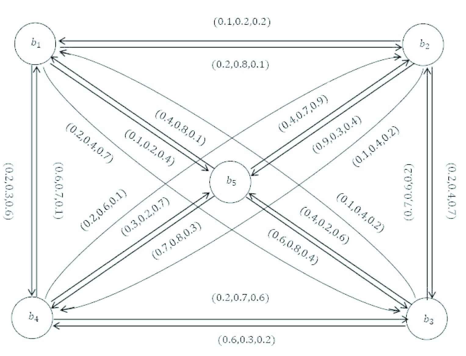
Data is converted in digraphs which shown in Figures 20–22. We can draw directed network corresponding to a collective SVNPR above, which is already shown in Figure 23. Under some conditions, Txy > 0.5, where x and y ranges from 1 to 5. Likewise, we have a partial diagram of all fused SVNPR which shown in Figure 24.
Single-valued neutrosophic diagraph D1.
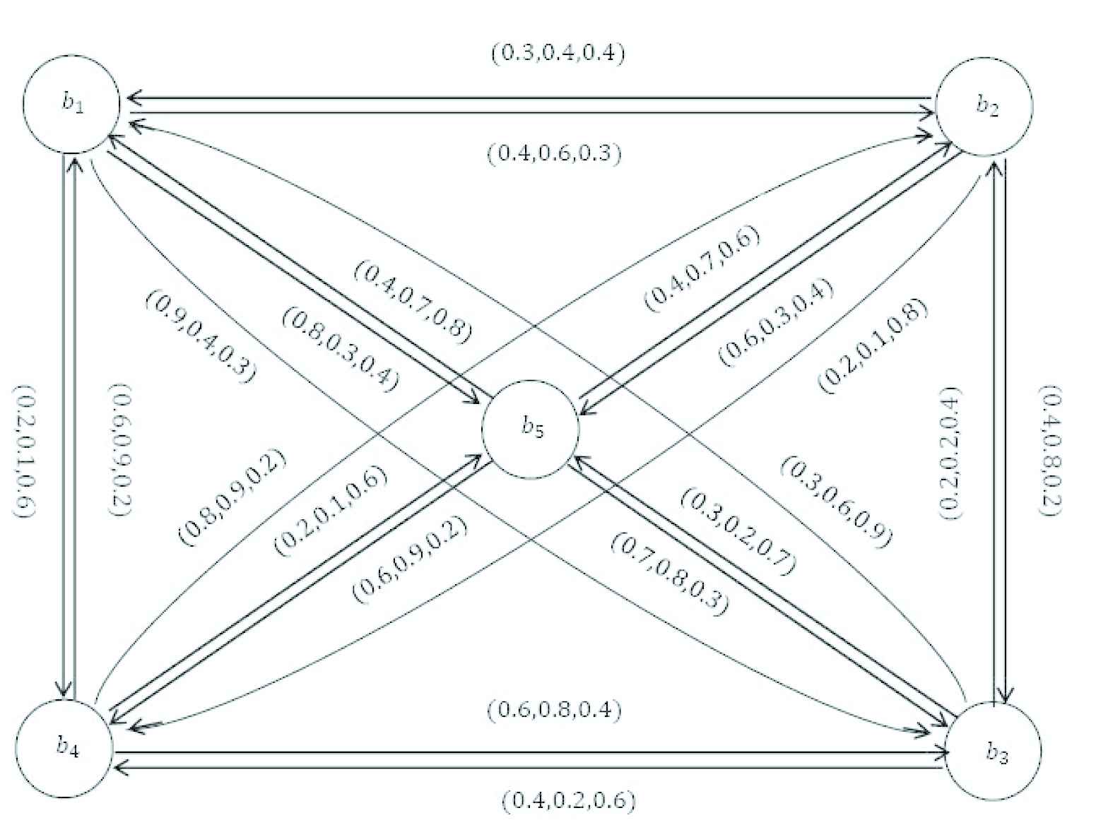
Single-valued neutrosophic diagraph D2.
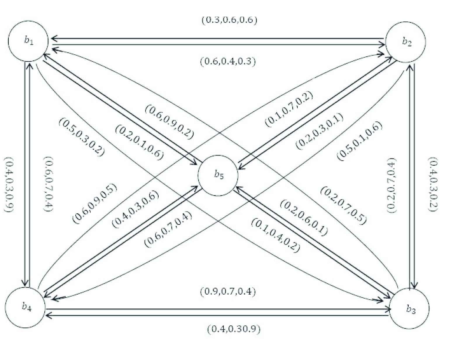
Single-valued neutrosophic diagraph D3.
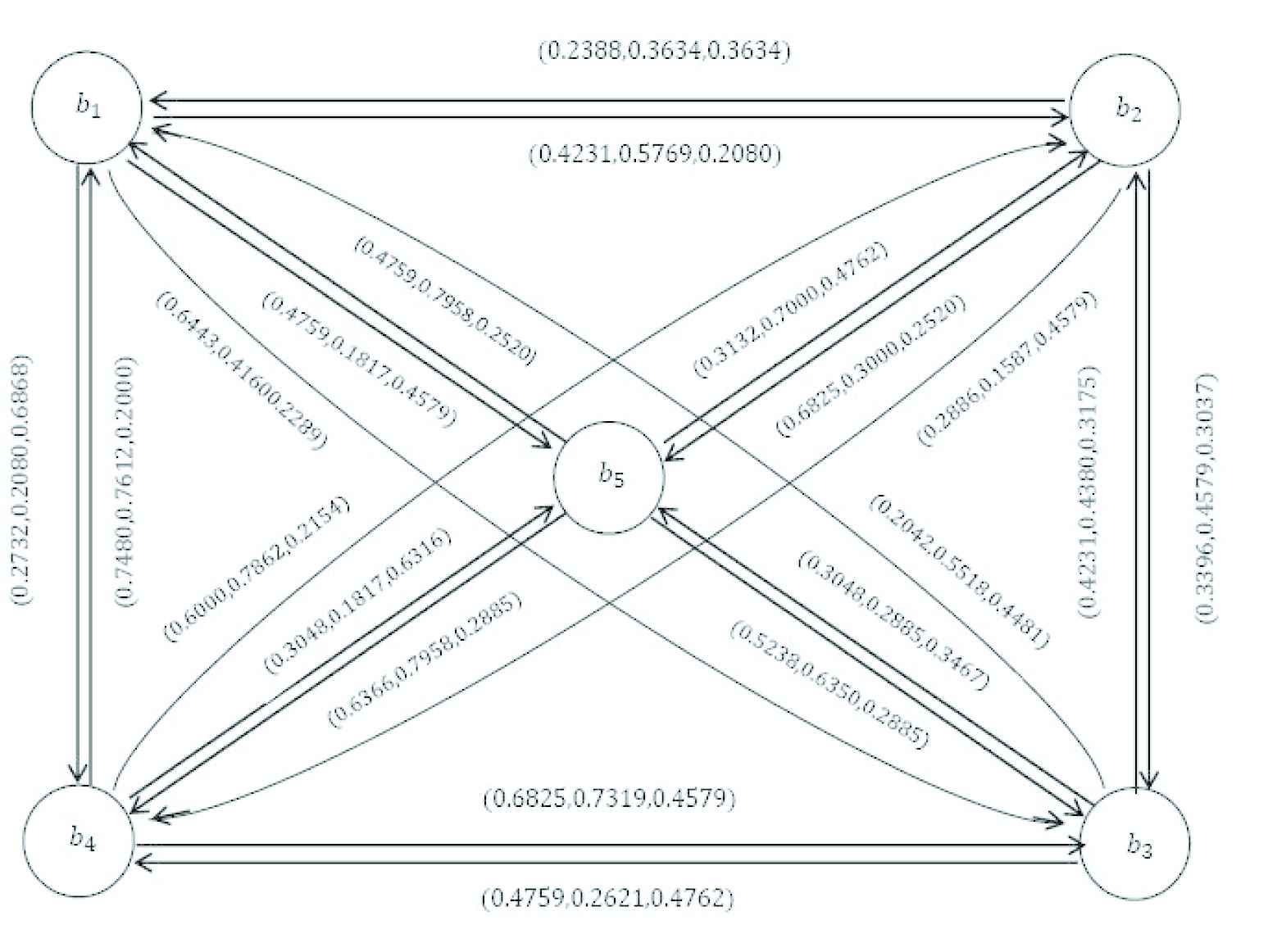
Directed network of all fused SVNPR.
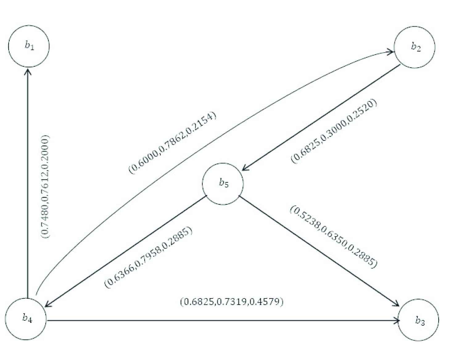
Partial directed network of all fused SVNPR.
We will find out the degrees which are denoted by out – dout – d (bx) with x = 1,2,3,4,5 of the whole criteria in a partial directed network as follows:
out – d(b1) = (0.0000, 0.0000, 0.0000)
out – d(b2) = (0.6825, 0.3000, 0.2520)
out – d(b3) = (0.0000, 0.0000, 0.0000)
out – d(b4) = (2.0305, 2.2793, 0.6733)
out – d(b5) = (1.1604, 1.4308, 0.5770) according to the membership degree rule of out – d(bx), x = 1, 2, 3, 4, 5, a ranking factors which is given below is obtained
5. CONCLUSION
The adaptability and equivalence of neutrosophic models are higher than fluffy models and intuitionistic fluffy models. A SVNG is broadly utilized in clinical sciences, financial matters, and logical designing. At the point when faltering happens in a genuine issue then the SVNG has a fundamental part to investigate the vulnerability since chart and the fluffy diagram don't think about the vulnerability among the relationship of the articles. We have examined the new properties on a SVNG known as the buildup item, maximal item, symmetric distinction, and dismissal of a chart. We likewise examined the thought with guides to discover the degree and absolute level of vertices of some specific charts. A few hypotheses of these diagrams were recently settled by utilizing the idea of degree and complete level of a vertex of a chart. Additionally, the hypotheses which were identified with these properties were demonstrated. Additionally, the fascinating and helpful use of a SVNG was examined which was a choice of reasonable organization by FAO. At last, a calculation which is the strategy of our application was introduced. Next, our motivation in future work is to introduce this idea on (1) complex bipolar-SVNG, (2) complex bipolar fuzzy graph, and (3) complex interval-valued fuzzy graph with their connected applications.
CONFLICTS OF INTEREST
The authors declare of no conflicts of interest.
AUTHORS' CONTRIBUTIONS
All authors have equal contribution.
ACKNOWLEDGMENTS
This work is supported by the Social Sciences Planning Projects of Zhejiang (21QNYC11ZD).
REFERENCES
Cite this article
TY  - JOUR
AU  - Shouzhen Zeng
AU  - Muhammad Shoaib
AU  - Shahbaz Ali
AU  - Florentin Smarandache
AU  - Hossein Rashmanlou
AU  - Farshid Mofidnakhaei
PY  - 2021
DA  - 2021/04/26
TI  - Certain Properties of Single-Valued Neutrosophic Graph With Application in Food and Agriculture Organization
JO  - International Journal of Computational Intelligence Systems
SP  - 1516
EP  - 1540
VL  - 14
IS  - 1
SN  - 1875-6883
UR  - https://doi.org/10.2991/ijcis.d.210413.001
DO  - 10.2991/ijcis.d.210413.001
ID  - Zeng2021
ER  -