
Distorted Vehicle Detection and Distance Estimation by Metric Learning-Based SSD
 , Yi Jin3, †, Shichao Kan1, 2, , Linna Zhang4, Yigang Cen1, 2, *, Wen Jin5
The first two authors (Fanghui Zhang and Yi Jin) contribute equally.
- DOI
- 10.2991/ijcis.d.210419.001How to use a DOI?
- Keywords
- Object detection; Vehicle distance estimation; Metric learning; Scalable overlapping partition-pooling
- Abstract
Object detection and distance estimation based on videos are important issues in advanced driver-sssistant system (ADAS). In practice, fisheye cameras are widely used to capture images with a large field of view, which will produce distorted image frames. But most of the object detection algorithms were designed for the nonfisheye camera videos without distortion, which is not suitable for the application of ADAS since one always expects the panorama stitching and object detection system should share one set of cameras. The research of vehicle detection based on fisheye cameras is relatively rare. In this paper, vehicle detection and distance estimation based on fisheye cameras are studied. First, a multi-scale partition preprocessing is proposed, which can enlarge the size of small targets to improve the detection accuracy of small targets. Second, parameters learned from the public datasets without distortion is transferred to our fisheye video dataset. Then metric learning-based single shot multibox detector (MLSSD) is proposed to improve the accuracy of distorted vehicle detection. Combining metric learning and SSD network, MLSSD can significantly reduce the missing and false detection rates. Moreover, a scalable overlapping partition pooling method is proposed to explore the relations among the adjacent features in a feature map. Finally, the distance between the driving vehicle and vehicles around this vehicle is estimated based on the object detection results by the method of marker points. Experimental results show that our proposed MLSSD network significantly outperforms other networks for distorted object detection.
- Copyright
- © 2021 The Authors. Published by Atlantis Press B.V.
- Open Access
- This is an open access article distributed under the CC BY-NC 4.0 license (http://creativecommons.org/licenses/by-nc/4.0/).
1. INTRODUCTION
In recent years, advanced driver-assistant system (ADAS) became a hot topic all over the world, which aims to help the driver avoid accidents according to different sensors such as lidar, cameras, etc. Object detection and vehicle distance estimation based on real-time videos are the important tasks of ADAS, which can directly show the situation surrounding the vehicle and provide an early warning to the driver. As the cost of hardware devices decreases and computing power increases, vehicle detection technologies based on computer vision have made great progress and are widely used in ADAS.
Vehicle detection made great progress in the last decade. Support vector machine (SVM) [1], was used for vehicle detection. By combining the histogram of oriented gradient (HOG) and Gabor features, a composite feature was proposed to express the vehicles [2]. Chang and Cho [3] proposed the online boosting method, which was robust for novel vehicle types and unfamiliar environments. With the prosperous usage of deep learning, different network structures [4] were proposed for objection detection, such as Faster R-CNN [5], SSD [6], YOLO [7]. They have been successfully applied for vehicle detection in recent years.
Most of the abovementioned algorithms are applied for images obtained by nonfisheye cameras. In the ADAS system, the panorama stitching and object detection system are expected to share a set of cameras. For the panorama stitching, fisheye cameras must be used to cover all angles surrounding the vehicle. Thus, object detection on the fisheye camera is an important task for the sake of saving hardware resources.
Although a fisheye camera can capture a large view angle of the image, the objects in the image will have significant distortion, which increases the difficulties for directly using the existed detection networks. Academically, there are some public vehicle detection datasets such as KITTI [8], DETRAC [9], COCO [10], and VOC [11]. But there is no public dataset of distorted images for vehicle detection so far. Based on the mainstream object detection framework, if one model is trained based on the public dataset while tested on the distorted images or videos, the accuracy of the test dataset will decrease significantly. Moreover, manually relabeling a large new training dataset of distorted images is very time-consuming and boring. Thus, how to utilize these existing public datasets for object detection with distorted images is one of our main research goals.
In this research project, a dataset with 12192 distortion images is constructed, which is denoted as the distorted vehicle dataset
However, the detection accuracy is low if we just simply transfer the parameters learned from the normal datasets to our distortion dataset. For example, some foreground vehicles are not detected and some background objects are wrongly detected as vehicles [12]. We recognize that the foreground can be distinguished from the background for both the public datasets and the distorted dataset by similarity measurement [13]. This motivates us to use metric learning to improve the detection accuracy by designing a metric loss function, which will shrink the intra-class distance while enlarge the inter-class distance. Beside, the performance of SSD for small object detection is poor [6]. Possible solutions for this problem are using high-resolution images or training the network with a multi-scale image pyramid method. But these methods will bring extra computational cost. Bharat et al. [14] presented an algorithm for efficient multi-scale training, which sampled low resolution chips from a multi-scale image pyramid to accelerate multi-scale training by a factor of three times.
In this paper, an end-to-end object detection framework is proposed for distorted vehicle detection and distance estimation, named as the metric learning-based single shot multibox detector (MLSSD). Two branches are included in the proposed MLSSD. One branch is the SSD network and another one is metric learning-based classification (MLC) network. Both of them share the first five convolutional layers of the VGG network. In addition, in order to improve the detection accuracy for small objects, a multi-scale partition preprocessing is added to select positive blocks for network training. The main contributions of this paper are as follows:
An object detection framework, named MLSSD, is proposed by combining the metric learning and SSD network. Also, a multi-scale partition pre-processing is added in front of the MLSSD to improve the detection accuracy for small objects.
Scalable overlapping partition pooling (SOPP) is proposed to explore the relations among the adjacent features in a feature map.
The distance between the driving vehicle and vehicles around this vehicle is estimated based on the object detection results by the method of marker points.
The effectiveness and superior performances of the proposed MLSSD framework are demonstrated for vehicle detection and distance estimation in the distorted driving videos. The rest of this paper is organized as follows. In Section 2, related works about object detection, metric learning, and transfer learning are reviewed. The proposed structure of MLSSD, multi-scale partition preprocessing, the generation of nonredundant samples, the SOPP method, the metric learning, and the vehicle distance estimation are presented in Section 3. In Section 4, algorithm implementation details, datasets, evaluation metrics, and the experimental results are presented. Section 5 concludes the paper.
2. RELATE WORK
In this paper, our work mainly involves three aspects, i.e., object detection [15,16], metric learning [17], and transfer learning [18]. Works related to them are reviewed in this section.
2.1. Object Detection
Starting from R-CNN [19], Girshick Ross introduced deep learning into the object detection field, and gradually improved it. Nowadays, all steps of object detection are unified under the deep learning framework, meanwhile, the accuracy and the speed are greatly improved.
The detector of object detection can be divided into two categories: the two-stage detector and the one-stage detector. A typical representative of the two-stage detector is Faster R-CNN [5], in which the region proposal network (RPN) is proposed, instead of the selective search to generate proposals. In Faster R-CNN, RPN, and Fast R-CNN are merged into a single network by sharing the convolutional layers to achieve end-to-end detection. It achieved better results compared with Fast R-CNN. The running time is greatly shortened while the accuracy is improved. Subsequently, its extended networks (such as RFCN [20] and Mask R-CNN [21]) are proposed to further improve the accuracy and speed.
A typical one-stage detector is the SSD network. SSD effectively combines the ideas of RPN and YOLO for target detection under multi-scale convolutional layers. The accuracy of SSD is higher than YOLO and the detection speed can reach 59 FPS.
In the past few years, SSD network and its extensions (such as DSOD [22], DSSD [23], STDN [24], and RFBNet [25]) were proposed to continue improving the object detection accuracy. The DSOD network combines the ideas of DenseNet and SSD to train the object dataset from the beginning. It does not require a pretrained model and a large amount of training data. However, the DSOD network is mainly working for special images, such as medical images with high accuracy. Its detection accuracy on other common datasets is far less than that of the most advanced algorithms such as RFBNet. By adding some additional layers to the SSD and adopting the encoding-decoding strategy, DSSD fused high-level content information and low-level feature maps to improve the detection accuracy. But the detection speed of DSSD is slower than SSD because the additional layers are added. The STDN network proposes an effective scale transfer module, and obtains a larger feature map by reducing the number of feature map channels. It improves the accuracy of small target detection. Because there are no additional parameters added, the speed is comparable to the SSD. RFBNet modifies the network structure of SSD by adding the RFB framework and proposing a receptive field block. It obtains better detection accuracy than SSD. Although these extension models of SSD continuous improving the detection accuracy and speed, the object detection accuracy is also need to be further improved.
2.2. Metric Learning
Metric learning has also made rapid progress in recent years. The goal of metric learning is to learn effective metrics by comparing the similarity of input image pairs, and finally makes the distance from the same classes smaller than the distance from different classes. It is widely used in image retrieval [26], pedestrian recognition, image classification, and target detection.
Metric learning can be divided into linear model and nonlinear model. The traditional metric learning methods [27,28] are to learn the linear Mahalanobis distance to measure the similarities among samples. For example, Schultz et al. [27] proposed a method that learns distance metrics from relative comparison using the SVM method. Globerson and Roweis [28] proposed an algorithm for learning quadratic Gaussian metrics by constructing a convex optimization problem, which attempts to map all samples in the same class to a single point, and makes samples in other classes infinitely far away from this point. The linear mapping method can be converted into a nonlinear model by the kernel expansion method [29–32]. Nowadays, deep learning is developing rapidly, and more and more researchers [33–41] use deep learning to learn the nonlinear model. Song et al. [13] proposed a method of distance measurement between samples by utilizing the advantages of batch in the network training, which upgrades the pairwise distance vector of samples in a batch to a distance matrix. In this way, the distance information of the samples is increased without increasing the batch size. Duan et al. [39] proposed a deep adversarial metric learning (DAML) framework to generate potential hard negative samples from observed samples, which are used as a complement to hard negative samples to learn more accurate distance metrics.
2.3. Transfer Learning
With the rapid development of deep learning, the demand for the amount of data is getting higher. When the data size for a specific application is small, transfer learning [42,43] can be used to obtain a good performance. Transfer learning and domain adaptation refer to the knowledge gained in one scenario and used in another to improve the performance. In short, a pretrained model is reused in another task. Yosinski et al. [43] presented an experimental illustration on how to transfer features in deep convolutional neural networks. When the target dataset is small and the parameters quantity is large, some network layers can be frozen. When the target dataset is large and the quantity of parameters is small, fine-tuning may produce better results. If the target dataset is very large, better results can be get without using transfer learning. In our work, our target dataset is the distorted dataset
3. PROPOSED METHOD
The whole framework of our proposed MLSSD is shown in Figure 1. For each image, six blocks are cropped from the original image and positive blocks are selected for training. MLSSD consists two parts as shown in Figure 1. The upper part is a MLC network, which is used to adjust the parameters of VGG-16 such that the foreground and background in the output feature maps of VGG-16 can be more distinguishable. The lower part of Figure 1 is SSD network using for object detection.
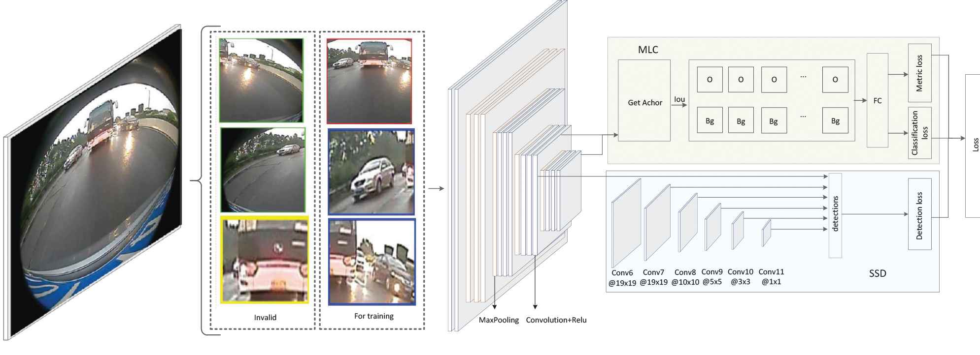
The framework of MLSSD.
3.1. Multi-Scale Partition Preprocessing
For an input image, usually, the background area occupies a large portion of the image. If the image is resized, large targets could become too larger or small targets could become too smaller [14], which will affect the detection performance greatly. To solve this problem, we propose a multi-scale partition preprocessing method to improve the detection accuracy of small targets, which uses 6 windows with different scales to partition the original image into 6 blocks. These 6 windows are responsible for cropping all targets with different scales into different blocks (small targets will be included in the small blocks and large targets will be included in the large blocks). After resizing these 6 blocks in a same scale, the small targets will be enlarged and large targets will be shrunk such that all target are almost in a same scale. Moreover, the blocks containing a relatively large portion of targets will be selected as positive blocks, and other blocks that containing a large portion of background will be removed. This preprocessing will reduce the difficulties of small target detection and the computational cost of large target detection. The details are introduced as follows.
3.1.1. Blocks generation
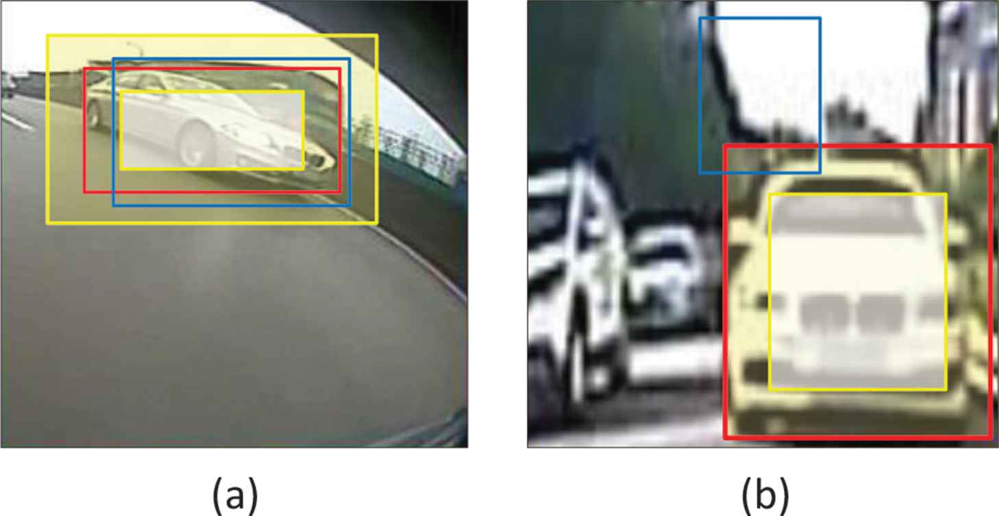
Six blocks with four different scales are selected in this paper. In Figure 2(a), the red and yellow blocks are used to detect large targets and small targets in the rear, respectively. It can be seen that all targets in the image will be included in these 6 blocks. The green and blue blocks are used to detect large and small targets respectively on both the left and right sides. Red and yellow blocks will cover all targets in the middle of the image. After these 6 blocks are cropped, they are resized into a unified size, as shown in Figure 2(b)–2(g). These six blocks are not all useful. For example, there is only one truncated target in Figure 2(f) and this target is fully included in Figure 2(d). Thus, Figure 2(f) can be removed.

Image blocks selection. (b)-(g) are six blocks cropped from the original image (a) (a yellow box, a red box, two blue boxes, and two green boxes). The small target vehicles on the left and right sides are enlarged in (b) and (f) by the blue boxes, and the small target vehicles on the rear are enlarged in (d) by the yellow box. Large vehicles on the left, in the middle and on the right are shrunk in (c), (e), and (g) by the green and red boxes.
3.1.2 The selection of positive blocks and negative blocks
For each block, we hope the object included in this block has an appropriate size. For example, both the yellow and red rectangles of Figure 2(a) consist of a white car. Obviously, the white car’s size is suitable for the yellow rectangle and too small for the red rectangle. When we select the training samples, the yellow block containing the ground-truth box of this car should be selected as a training sample. Thus, for each block, we can define a desired area range to indicate the appropriate object size for each block, denoted as
3.2. Metric Learning-Based Classification
In our proposed MLSSD, MLC is utilized for adjusting the parameters of the feature extraction network (i.e., VGG-16) in the training stage, such that the features obtained by VGG-16 can be more distinguishable for the foreground and background objects. MLC combining the metric loss and classification loss, as shown in the upper right part of Figure 1. The metric loss will enlarge the distance between the object sample features and the background sample features, and shrink the distances within the same category. The classification loss is responsible for MLC, and SSD networks are trained alternatively to optimize the parameters of the whole network. The MLC network structure is as follows.
3.2.1. Nonredundant object samples
In Figure 1, the anchors are generated by the RPN [5] after conv5-3 of VGG-16, as shown in Figure 3. Figure 3(a) is a 32 × 32 feature map of VGG 5-3. Each feature point of a feature map in Figure 3(a) is related to a receptive field of the original image, as shown in Figure 3(b). Ren et al. [5] used three scales and three aspect ratios at each receptive field. According to the length-to-width ratio of vehicles in the images and the distance between the vehicles and the camera, five scales with box areas of
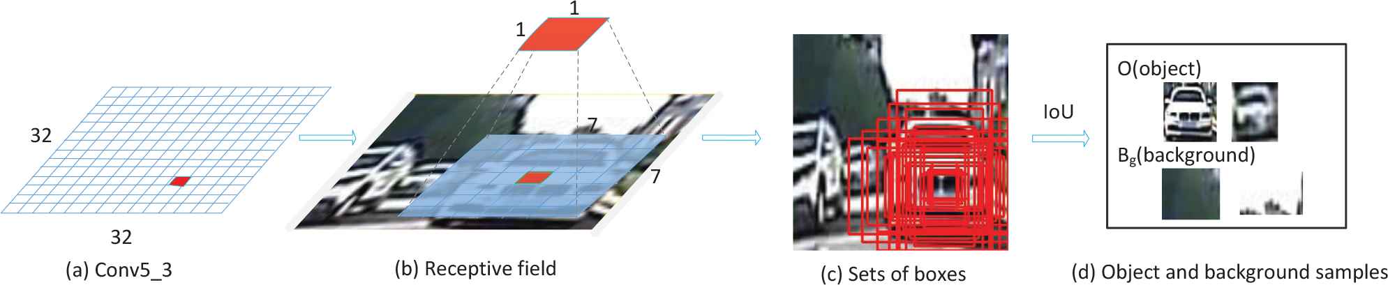
Object and background samples mining method in MLC.
According to the above operations, many samples determined by the anchors of object and background can be obtained with high redundant information. The nonmaximal suppression method is employed here to reduce the redundant samples. Specifically, we select the bounding box
3.2.2. SOPP for feature extraction
Spatial pyramid pooling (SPP) [44] is a widely used method in object detection networks, which transforms different scale samples into the same size, as shown in Figure 4. Features A, B, C are three image patches, which are 128 × 128 pixels, 128 × 84 pixels, and 64 × 64 pixels, respectively. Because of three times pooling, the feature map sizes in conv4-3 or conv5-3 of the VGG net corresponding to A,B, C are 16 × 16, 16 × 11, and 8 × 8, respectively, see Figure 4(b). Then the feature maps are partitioned into 16, 4, and 1 blocks, respectively in Figure 4(c). The red, blue, and green blocks respectively denote one block in these three cases. The max value of each block can be found. Concatenating all the max values of these 21 blocks, a 21-dimensional feature vector can be finally obtained.
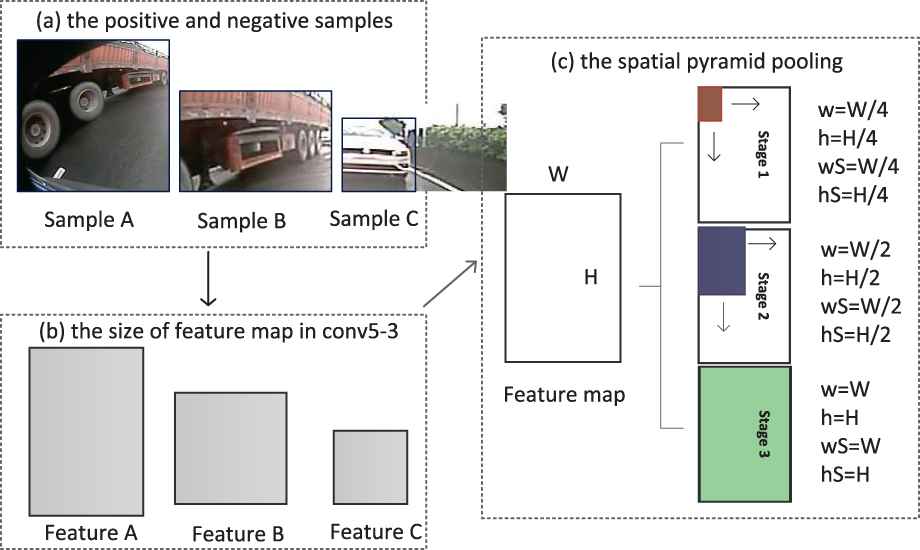
The feature spatial pyramid of different size samples.
By Figure 4(c), the adjacent features obtained after SPP lack of associations because that the nonoverlapping division method is adopted. Inspired by the scalable overlapping partition (SOP) method [45], we propose SOPP to establish the connections among adjacent features. The whole process of SOPP is shown in Figure 5, which can transform feature maps with different sizes into a unified form with fixed dimensionality. Suppose the size of a feature map is W × H, in stage 1, the maximum value of the whole feature map is extracted as a feature value. In stage 2, the feature map is divided into 3 blocks by a sliding window (the window size is W ×, as the blue block shown in Figure 5) with overlap of H/4. The size of the sliding window decides the size of pooling areas. Therefore, 3 feature values can be obtained by extracting the maximum values of these 3 blocks. Stage 3 is similar to stage 2, the difference is that the sliding window size is changed as

The scalable overlapping partition pooling.
In our network, the feature maps in the convolutional layers 4-3 and 5-3 of VGG-16 are used for both the MLC and SSD. As a result, a 16384-dimensional feature vector can be obtained after the SOPP, i.e.,
3.2.3. Metric loss
In the MLC, when a sample
For the images we obtained by the fisheye camera, the background is complex without vehicle information, or only contains a little of very small vehicles at the far-end of camera. As our goal is vehicle detection, the differences among the foreground samples, and differences between the foreground and background samples are more concerned rather than the similarities among the background samples. Thus, the loss function can be only defined based on all of the object and background samples in the training set:
3.2.4. Multi-loss function
In the MLC, both metric loss and classification loss are used. This multi-loss function will force the distances of two samples in the same class to be less than the distance from different classes. Also, it can classify samples into their correct categories. For the classification loss, softmax cross-entropy classification loss is used. Training convolutional neural networks through a joint loss function is a very effective way to improve the performance of the network. The multi-loss function is defined as follows:
3.3. Single Shot Multibox Detector
The second network branch of the MLSSD is the SSD network, as shown in the lower right part of Figure 1. VGG network is used as the basic network and followed by an auxiliary structure for object detection. SSD uses both high-level feature maps and underlying feature maps simultaneously for object detection. Moreover, feature maps of different layers are used to detect objects at different scales. More details can be found [6].
3.4. Distance Estimation
Estimating the distance between the driving vehicle and vehicles around this vehicle is an important step in ADAS. The green points in Figure 6(a) are marker points, where the distance between any two adjacent marker points is 30cm. Figure 6(b) is the nondistorted projection of Figure 6(a). The areas beyond marker points are inestimable. In this paper, we stipulate that the midpoint of a vehicle detection box’s bottom line is a detection point (star point), as shown in Figure 6(b). The distance from a detection point to the midpoint of the vehicle (red line’s distance in Figure 6(b) needs to be calculated. Firstly, the detection point of a target vehicle should be mapped to a marker point using leaky Euclidean distance. The leaky Euclidean distance means that the index of a mapping point is obtained only from the shortest distance in the transverse and longitudinal direction, respectively. Secondly, the distance and relative azimuth between the mapping point and the vehicle’s midpoint are calculated by using the index of the mapping point obtained in the previous step. If the relative azimuth is within the angle of the two blue dashed lines, a vehicle is behind the driving vehicle. Otherwise, a vehicle is on the left or right side. Finally, if a vehicle on the left or right of the driving vehicle, the left button point or right button point of a vehicle’s bounding box is a detection point. The distance can be calculated according to the second step. Otherwise, the distance is the result of the second step.
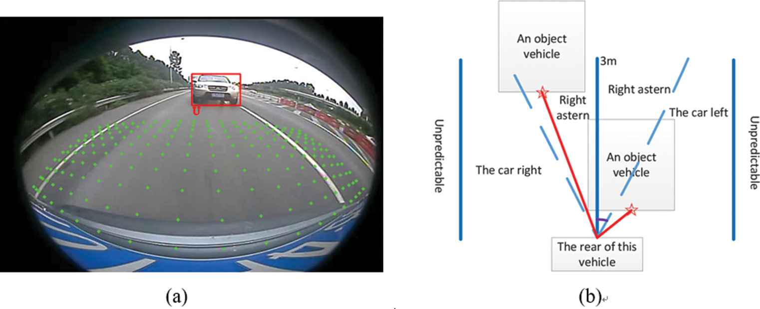
The method of the distance estimation. Here, in (a), the green points in the right picture are marker points and (b) is the nondistorted projection of (a). In (b), the length of blue lines is 3 meters, the distance from the midpoint of this vehicle to the blue lines on the left and right is 3 meters, respectively.
4. EXPERIMENTS AND RESULTS
4.1. Implementation Details
4.1.1. The distorted vehicle dataset
Because we want the object detection system and the panorama stitching system to share the same set of cameras, the objects in the images are all distorted. To the best of our knowledge, there is no such public vehicle dataset. Therefore, we manually labeled the images and form a distorted vehicle dataset, denoted as dataset
Because the amount of the distorted vehicle dataset
According to the above discussions, we construct another vehicle dataset that only contains normal images, denoted as
4.1.2. Network training
First, the SSD is parameterized by a pretrained model based on ImageNet. Then the dataset
The convolutional layers of SSD shared with MLC in Figure 1 are initialized by the model
Algorithm 1: The training process of the our network
Input: Images in the distorted vehicle dataset.
Output: The trained network.
Initialize: Initialize the convolutional layers shared by SSD and MLC networks in MLSSD by the pre-trained model
Step 1: Train the MLC network by fixing the network parameters of the SSD branch. The network parameters of MLC network are modified by the back propagation algorithm.
Step 2: Train the SSD network by fixing the network parameters of the MLC branch.
Step 3: Repeat Step 1, Step 2 until convergence.
According to the Section 3.2.1, nonredundant object and background samples can be obtained. There are two cases needed to be considered: (1) The object samples obtained in the frame is less than 2, which will lead to the result that the
Get a fixed number of samples.
In our training process, transfer learning is used, which converges quickly as shown in Figure 8. We evaluate detection mean Average Precision (mAP), because this is the actual metric for object detection [8]. At the testing stage, the mAP with transfer learning is 90.5%, which is 3.8% higher than the accuracy obtained without transfer learning.
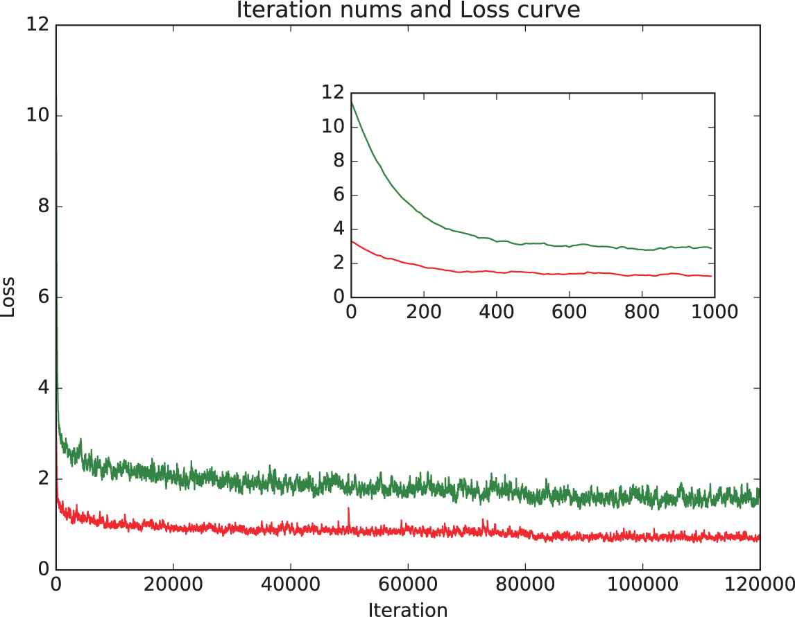
Iteration times and loss values. Here, the red curve is the loss curve with transfer learning, and the green curve is the loss curve without transfer learning.
4.2. Comparisons with Other Methods
Table 1 shows the comparison results of five networks: proposed MLSSD, SSD, Faster R-CNN, YOLO, and KittiBox. For the speed comparison (including data reading and display), the five networks are tested with and without GPU. It can be seen that Faster R-CNN is the slowest, while KittiBox and YOLO are the fastest. Although our proposed MLSSD is trained by adjusting the parameters of MLC and SSD branches alternately, only the SSD branch is used for testing. Because six blocks in an image need to be tested in MLSSD, our algorithm is slower at the testing stage than SSD. But, our network achieves the highest mAP, as high as 90.5%, which is 5.3% higher than SSD. The YOLO has the lowest mAP of 81.2%.
| Proposed MLSSD | SSD | Faster R-CNN | YOLO | KittiBox | |
|---|---|---|---|---|---|
| mAP | 90.5% | 85.2% | 89.7% | 81.2% | 82.6% |
| Speed-CPU | 1.7 fps | 3fps | 0.2fps | 7fps | 7fps |
| Speed-GTx1060 | 6.4fps | 12fps | 0.8fps | 30fps | 30fps |
The mAP and speed of different networks in the distorted vehicle dataset
Although the mAP of Faster R-CNN is only lower than our MLSSD of 0.8%, it is too slow to realize real-time detection. These results show that our proposed MLSSD achieves good performance by balancing accuracy and speed. Part of the detection results of the MLSSD are shown in Figure 9.
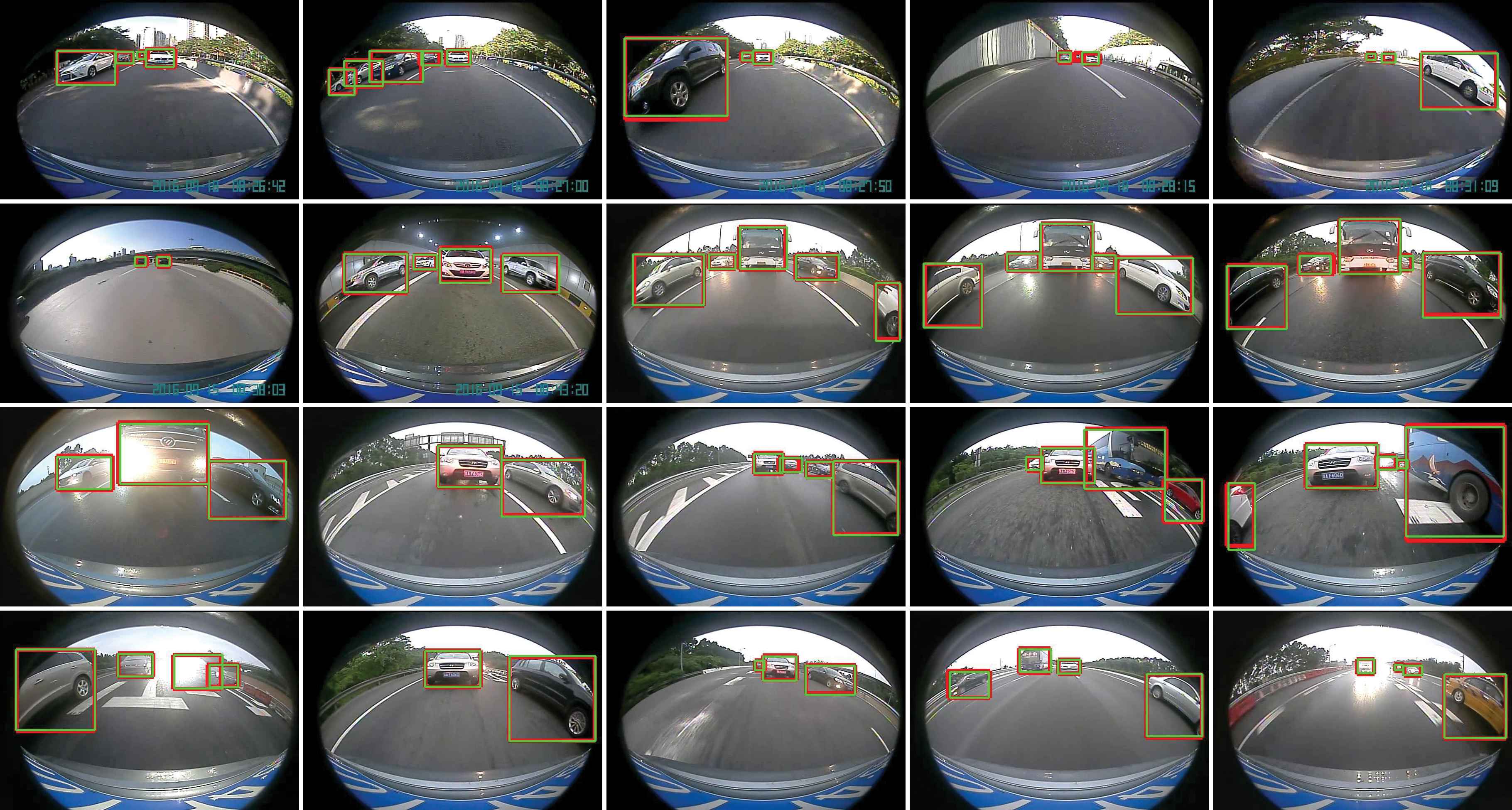
Some vehicle detection results obtained by our proposed MLSSD. The red and green boxes shown in the images are our detection results and the ground truth, respectively.
4.3. Experiments on the UA-DETRAC Dataset
In order to verify the robustness of our proposed network, the experiments are performed on the UA-DETRAC [9] dataset, which contains 82085 training images and 56167 test images. The mAPs of the proposed MLSSD, SSD, Faster R-CNN, YOLO, and KittiBox are 73.4, 71.0, 72.7, 58.7, and 60.0, respectively. The speeds tested in GTX1060 are 4fps, 7fps, 0.3fps, 16fps, and 16fps, respectively. It can be seen that the performance of the proposed MLSSD is still good.
4.4. Vehicle Distance Estimation Results
After getting the detection results by using the MLSSD method, the method of the vehicle distance estimation is used to estimate the distance from the driving vehicle to target vehicles. When the target vehicle is within three meters away from the driving vehicle, the distance is calculated in this paper. When the distance exceeds three meters, the distance is unpredictable. The azimuth of the target vehicle is given according to the position relationship between the target vehicle and this vehicle. The results are shown in Figure 10. In addition, in order to compute the accuracy of the estimated distance obtained by our algorithm, we parked the test vehicle in a parking area and manually measure the real distances between our vehicle and others. We manually measured 100 distances in total. The final results are shown in Table 2. Here we only show the average distance errors between the distance obtained by our algorithm and the real distance.
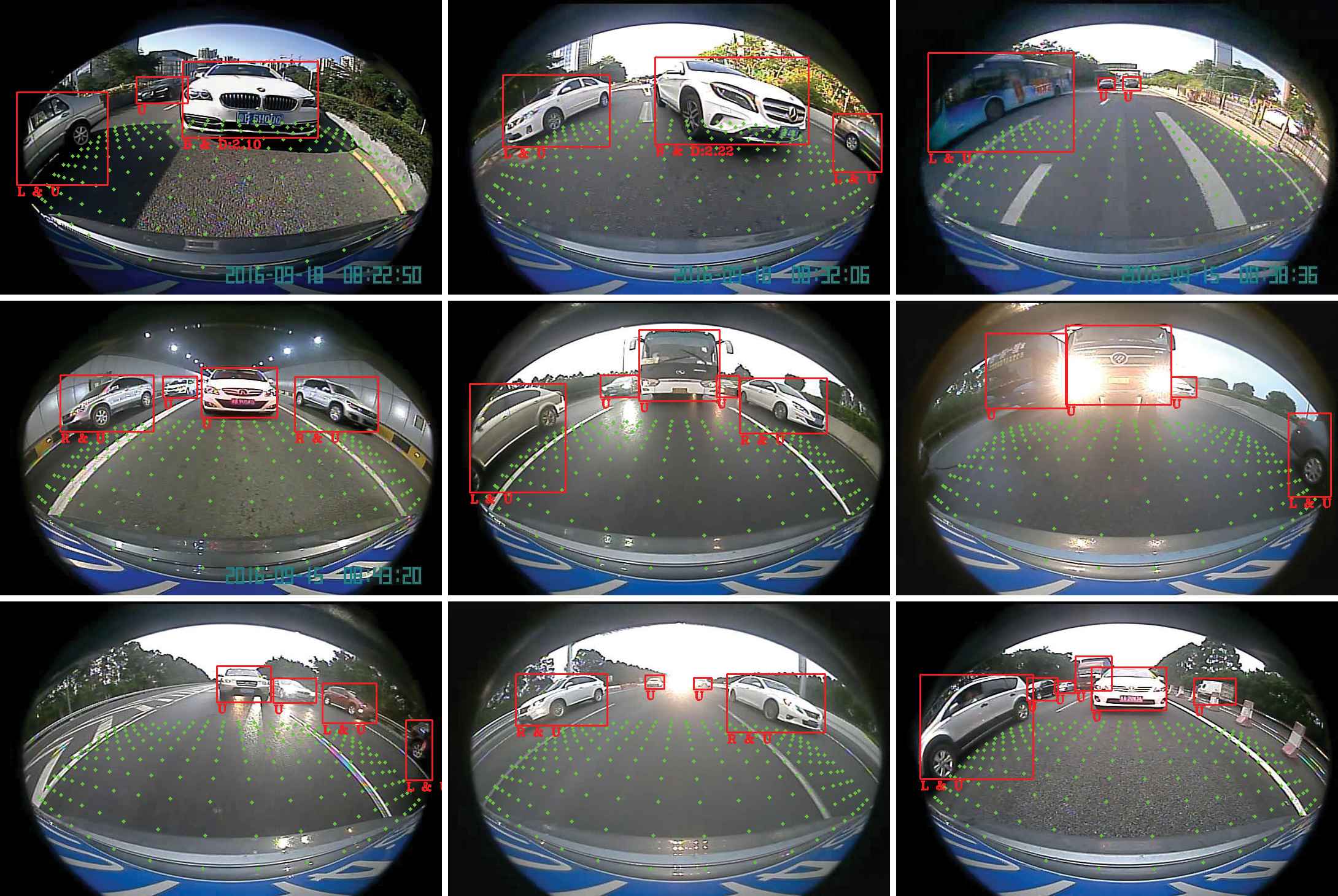
Results of the vehicle distance estimation. Here, the red boxes are the results of the vehicle detection. The green points are the marker points. U means the distance from this vehicle to a vehicle is unpredictable. B(L or R) means a vehicle is behind (on the left of or on the right of) the vehicle. D stands for the distance.
| Distance | <1 m | 1 |
2 |
|---|---|---|---|
| Error | 0.08 | 0.17 | 0.33 |
The average distance errors.
5. CONCLUSIONS
In this paper, MLSSD network is proposed to improve the accuracy for distorted vehicle detection based on fisheye camera videos, which combines the metric learning and SSD network. In our algorithm, a multi-scale partition preprocessing is proposed to enlarge the size of small targets to improve the detection accuracy of small targets. In addition, SOPP is proposed to explore the relations among the adjacent features in a feature map. Finally, the distance between the driving vehicle and targets around this vehicle can be roughly estimated based on the object detection results by the method of marker points. Our approach can be trained end-to-end and achieved a good performance in the distorted vehicle dataset.
CONFLICTS OF INTEREST
The authors declare they have no conflicts of interest.
AUTHORS' CONTRIBUTIONS
FZ, SK, and YC conceived and designed the study. FZ and WJ made the vehicle dataset. FZ and YJ wrote the paper. YC, YJ and LZ reviewed and edited the manuscript. All authors discussed the results and revised the manuscript.
ACKNOWLEDGMENTS
This work was supported in part by the National Key R&D Program of China under Grant 2019YFB2204200; in part by the National Natural Science Foundation of China under Grant 61872034, Grant 61972030, Grant 62062021, and Grant 62011530042; in part by the Beijing Municipal Natural Science Foundation under Grant 4202055; in part by the Natural Science Foundation of Guizhou Province under Grant [2019]1064.
REFERENCES
Cite this article
TY  - JOUR
AU  - Fanghui Zhang
AU  - Yi Jin
AU  - Shichao Kan
AU  - Linna Zhang
AU  - Yigang Cen
AU  - Wen Jin
PY  - 2021
DA  - 2021/04/28
TI  - Distorted Vehicle Detection and Distance Estimation by Metric Learning-Based SSD
JO  - International Journal of Computational Intelligence Systems
SP  - 1426
EP  - 1437
VL  - 14
IS  - 1
SN  - 1875-6883
UR  - https://doi.org/10.2991/ijcis.d.210419.001
DO  - 10.2991/ijcis.d.210419.001
ID  - Zhang2021
ER  -