
Applying Meta-Heuristics Algorithm to Solve Assembly Line Balancing Problem with Labor Skill Level in Garment Industry
 , Ping-Shun Chen2, Jr-Fong Dang3, *, Sung-Lien Kang4, Li-Jen Cheng2
- DOI
- 10.2991/ijcis.d.210420.002How to use a DOI?
- Keywords
- Assembly line balancing problem; Toyota sewing system; Tabu search; Simulated annealing
- Abstract
This research investigates how to properly place garment industry workers to work stations in the assembly line to achieve a more balanced production and to reduce the production cycle time. We simulate the assembly line balancing problem via staff assignments. In our research, we conduct a comparative case study and implement our own simulation. The experiments are designed with both single- and multitasking modes. Each experiment is carried out for 10 runs. Finally, we compare our results obtained among constructive greedy, tabu search and simulated annealing. We find that tabu search algorithm is better than simulated annealing on the problem of staff assignment. Meanwhile, we also observe that if we adjust 30% labor force from single task into multitasking mode, the assembly line performance deteriorates. This case is accentuated for workers with disparate skill levels for different tasks.
- Copyright
- © 2021 The Authors. Published by Atlantis Press B.V.
- Open Access
- This is an open access article distributed under the CC BY-NC 4.0 license (http://creativecommons.org/licenses/by-nc/4.0/).
1. INTRODUCTION
Nowadays, the garment manufacturing industries are facing numerous challenges and intense market competition. For example, the industry is struggling with a urgent demand to raise the production efficiency while reduce the costs to gain the competitive edge. Furthermore, garment industries can be characterized with the mass-produced process and labor-intensive production. As the consequence, manufacturers would need to plan well the task placement and staff allocation at the early stage as to meet the customers’ requirements. Usually, the production process of garment manufacturing industries is executed in a sequential manner. Figure 1 shows that the general process can consist of the raw material selection, material inspection, sample production, cutting, sewing, ironing, packing, and so on. Please note that the steps from cutting to ironing are mostly labor-intensive. Also, the sequential relationship between the steps enables the production process to be treated as the assembly line model.
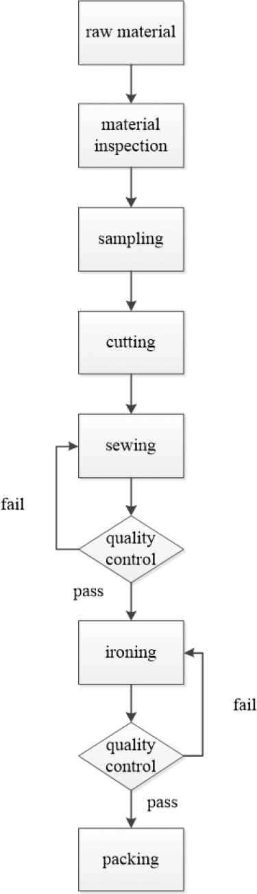
Garment manufacturing production process.
In the garment industry, the production quantity per day has to comply with the daily order in the industry. As a result, the assembly line layout can be a major factor and greatly impacts the production output. Additionally, the load distribution at each assembly line workstation may affect productivity. Therefore, the output rate of the assembly line would determine the balancing condition for each workstation and further influence production costs and customer satisfaction. The assembly line balancing (ALB) problem has been studied by enterprises for many decades. The ALB model ensures that the staff assignment balances the whole production process in order to effectively reduce the production time or idle time. To meet the ALB, employees' mastery of skills at each task would be considered as an indicator. However, there are few studies investigating into the multifunctional (multitasking) workers with multiple levels of skills working at work stations. Our research incorporates the concept of Toyota Sewing System (TSS) derived from the Toyota Production System (TPS) for clothing or footwear industry. TSS is credited with less floor space, flexibility and better working environment [1]. TSS is featured with a U-shaped assembly line and teams of workers making garments on a single-piece flow basis. Employees move between tasks and pass pieces of garments to the next employees as soon as they become available to process more products. The Toyota sewing machine system is shown in Figure 2 where sewing machines are represented by rectangle symbols while employees are labeled alphabetically.
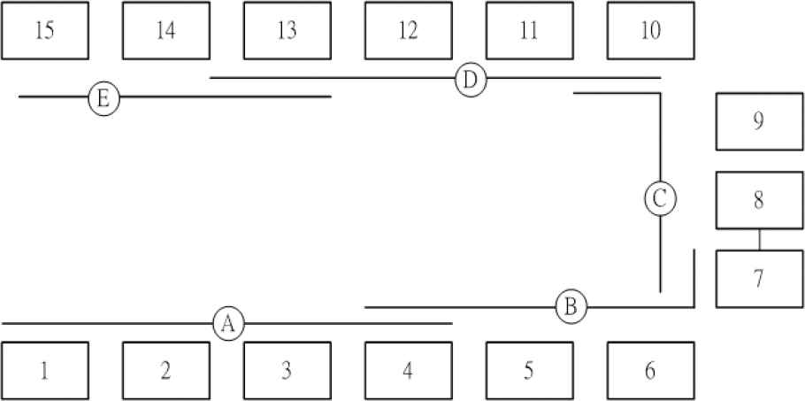
Toyota sewing machine planning system schematic.
As mentioned earlier, the labor-intensive feature of garment industry would be studied. Chan et al. [2] state that the skill and experience of supervisors can be treated as the important factor in controlling the production line and therefore improve the performance. Similar, Guo et al. [3] point out that the performance of the job shop mainly depends on supervisor’s experience and knowledge. Aǧrali et al. [4] develop their employee scheduling model considering the employee skill levels. To solve the problem within a reasonable amount of time, Aǧrali et al. [4] considers reformulation strategy. Dekena et al. [5] claim that the employees place the great impact on productivity and flexibility of the production system. They develop the production plan adopting the employee competence. Chen et al. [6] highlight that there is growing pressure in the skilled labor market. Chen et al. [6] proposes the model where the technicians must complete the given tasks within the time period and then gain the experiences. As such, technicians can be assigned to the job in the future. Wang et al. [7] study the problem of the employee competence in precast production planning. Furthermore, they propose a competence-based model to optimize the worker allocation. Chen et al. [8] address a multi-skill project scheduling problem for IT product development. In their research [8], the project is divided into multiple projects which are completed by a skilled employee. To solve the scheduling problem, they proposed a multi-objective nonlinear mixed integer programming model. This research takes into consideration of employees’ skill proficiency at performing tasks, multifunctional employees and cell formation to minimize the production cycle time. Also, we adopt another manner to calculate the cycle time different from the previous studies and further consider the workers’ skills to reflect the real-world situation. We find that the production time can be effectively reduced with a better personnel assignment and a preferred mode of production system.
2. RELATED WORKS
In this section, there are two main parts: ALB and TPS together with its extension TSS. The first part would introduce ALB problem and meta-heuristic algorithm. Then the TPS and TSS would provide readers with the production process approaches. Based on the aforementioned research, we develop our solution algorithm and enhance the solution procedure.
2.1. Assembly Line Balancing
Assembly line is an arrangement of workers, machines and equipment in which the product being assembled passes consecutively from operation to operation until completed. Furthermore, the ALB can be considered as one of the classical problems in assembly line and occurs frequently in the manufacturing industry [9,10]. Suer [11] states that ALB operates with precedence relationship to assign a number of operators or machines to each operation of an assembly line to meet the required production rate with a minimum idle time and to keep a leveled workstation time at each operation. In general, ALB includes Simple Assembly Line Balancing Problem (SALBP) and General Assembly Line Balancing Problem (GALBP). The SALBP can be divided into several categories [12]. That is, SALBP – 1, SALBP – 2, SALBP – E and SALBP – F. Note that the objective function of those SALBP is to minimize the idle time at the assembly line. As a result, researchers usually intend to obtain a total minimal idle time at each workstation in the assembly line under different production models or resource allocation. Regarding GALBP, Scholl and Klein [12] categorize it as Mixed ALB Problem (MALBP/MSP) and U-type ALB Problem (UALBP). Furthermore, ALB problem and its variants are considered to be NP-hard. This encourages one to apply meta-heuristic algorithms to derive the approximately optimal solutions due to its feature reducing solution space to accelerate the solution process. There are several meta-heuristic algorithms such as genetic algorithm (GA), tabu search (TS), simulated annealing (SA), and so on. Chan et al. [2] solve SALBP-E in garment industry by utilizing GA. In their solution procedure, they consider the skill level of the workers at each machine station and adopt the filtering mechanism of GA to properly assign workers to different station to reduce the total idle time and improve the production efficiency. Lin [13] employs GA to derive the optimal solutions of the shortest movement path of the single-row machine layout problem. The author applies a two-dimensional matrix to mark the movement distance of each machine and its sequence priority. Then the movement distance and suitability degree can be obtained by mathematical calculations of permutations and combinations. Suwannarongsri and Puangdownreong [14] propose a TS method to reduce the work load for the solving of the ALB problem. Given the cycle time and the number of workstations being fixed, the proposed method can not only maximize workstation load reduction but also cut down the idle time if machines are sectorized into different workstations based on the TS method. Dinh and Nguyen [15] develop three different approaches, exhaustive search, SA and SA with greedy, to solve ALB problem and further indicate that SA is the best one in terms of both accuracy and running time. Xu et al. [16] adopt an adaptive ant colony (AAC) algorithm with modifications to solve ALB problem. They define an objective function for minimizing the smoothness index measuring the difference among worktime and the targeted cycle time of each workstation on an assembly line. Quyen et al. [17] propose a hybrid genetic algorithm (HGA) to solve the resource -constrained assembly line balancing problem (RCALBP) in the sewing line of a footwear manufacturing plant. In their algorithm, the initial solution can be derived by the priority rule-based method (PRBM) in the first stage and then the solution is obtained by GA in the second stage. Gansterer and Hartl [18] consider balancing problems of one- and two-sided assembly lines with real-world constraints. The GA is utilized to solve the problem and then compare the performance of GA with TS by a set of larger test cases. They further show that GA outperforms a specific differential evolution (DE) algorithm and TS. Dang and Pham [19] utilize discrete event simulation (DES) to depict the performance measure and then integrate the adaptive large neighborhood search (ALNS) heuristic into the model to derive the solution. The authors conduct a footwear manufacturing factor with real data as the case study to see the proposed algorithm capability. Pereira [20] enhances the multi-Hoffmann heuristic to solve the ALB problem and further shows that its performance better than previous studies based on the results. He also validates the algorithm by implementing the model in the clothing company. Bautista et al. [21] propose their model maximizing the comfort of operators in mixed-model assembly lines. They further utilize mixed integer linear programming (MILP) and greedy randomized adaptive search procedure (GRASP) to derive the solutions. The authors state that even though the MILP provides the best solution, the results obtained by GRASP are comparative. As we can see, there are lots of papers solving the ALB problem by employing the meta-heuristic method. In this paper, we take a different approach of involving employee assignment to calculate cycle time in our research for garment industry, which differs from the existing approach of calculating cycle time. Also, the factor of workers’ skills is considered to reflect the real world.
2.2. Toyota Production System
In our research, we adopt TPS as one of our production process approaches to solve the ALB problem due to its U-shape feature. Pujo et al. [22] indicate that U-shaped layout is always at least efficient than an equivalent linear cell. Additionally, the TPS is developed by Taiichi Ohno, Shigeo Shingo and Eiji Toyoda between 1948 and 1975. The main objectives of TPS are to design for reducing cost, improving productivity, and thus eliminating wastes such as excess inventory, redundant human resources, and so on.
2.2.1. Toyota Sewing System
TSS is the extension of the just-in-time (JIT) production concept. TSS assists the garment industry in accepting the cellular manufacturing concept. The worker serving at the U-shape production line can operate multiple machines concurrently. The workers normally move counterclockwise to operate in a cell. When a worker completed his/her own jobs while his/her previous coworker delayed, this worker would adjust the direction and move clockwise to help the previous worker. Therefore, we may need to keep the production in the cells smooth and flexible. TSS production method is shown as Figure 3 [1].
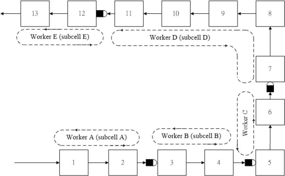
TSS production method [1].
In Figure 3, TSS assigns 3 to 5 workers to operate 13 machine stations. The workers can execute their jobs following the production process introduced above while achieve an effective balanced status. The workers can collaborate each other flexibly to minimize the idle time [1].
3. RESEARCH METHODS
In this section, we would introduce the limitations, formulation and the meta-heuristics algorithms applied in the model.
3.1. Research Definition and Limitations
In this research, we focus on the assignment problem of multiple tasks and different workers’ skill proficiency. Based on TPS, we modify one part of production process to the cell layout to solve the minimal cycle time of work.
3.1.1. The basic assumption
This study aims to solve the ALB problem in the garment industry. We make some assumptions about the issues and limitations for our research due to the cellular manufacturing concept. The basic assumptions and limitations are presented in the following bullets:
Workers have a specified skill proficiency for each task.
Each task is associated with the standard allowable minutes for the example of male short-sleeved shirt in the garment industry.
Operating processes observe the precedence relationship.
The worker’s operating routes cannot be crossed in each subcell.
Some production processes are not necessary classified as multitasking as depicted in the precedence relationship graph.
3.2. Mathematical Model
In our mathematical model, the objective function is to minimize the maximum cycle time.
Subject to
tj: the completion time of task j
mjk: task j assigned to work station k
C: cycle time
pj: task i precedes task j
In (1), we calculate the working hours for each workstation and select a largest working time as the cycle time. Then our study selects a minimum working cycle time of the combinations. Equation (2) is the constraint that each work station must be assigned to at least one worker. Equation (3) states the preceding relationship of tasks. For example, task i must be operated before task j; we use work stations to sectorize the positions of tasks that task i is in the work station that must be processed prior to that work station where task j is located. Equation (4) indicates the 0–1 variable; mjk is 1 if task j is assigned to work station k, 0 otherwise.
3.3. Cycle Time Calculation
In this research, the calculation of the cycle time is the main objective. One can derive the cycle time by selecting the longest completion time among the work stations as the completion time of the entire work. When we calculate the working cycle time, we have to make sure the number of tasks, work stations and working time for each task.
3.3.1. Placement of tasks
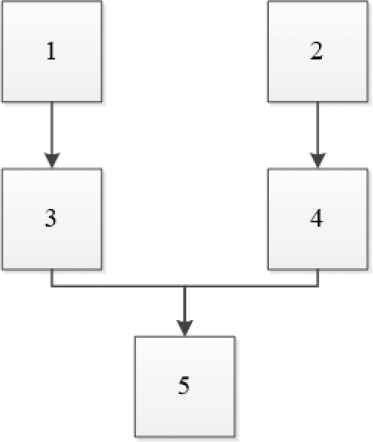
Based on the assumption as described earlier, we start to place tasks into the stations according the precedence relationship of the tasks. This approach is in accordance with the “most followers” decision rules of assigning the work element or task to a work station to satisfy the precedence requirements [23]. For example, task 1 is performed before task 3, while task 2 before task 4; task 5 is operated later than all tasks. The precedence relationship of tasks is shown as Figure 4.
Precedence relationship of task arrangement.
Once we have the above relationship among tasks, we put tasks into each station. We put 5 tasks into three different stations. First, we put the tasks without predecessors into a station. That is, we put task 1 and task 2 into station 1, and then we may put succeeding tasks of 3 and 4 into the next workstation. In the final stage, we put the last task 5 into the third station. Next, we calculate the completion time at each station, and the calculating of the cycle time is to select the longest station completion time as the cycle time. The layout of the tasks may not be optimized initially for cycle time reduction. The tasks at different work stations would then be readjusted to reduce the cycle time. During the process of readjustment, the precedence relationship must be observed among tasks. For example, we utilize Figure 4 to illustrate that task 3 or task 4 may be moved to work station 1. However, it is subject to the constraint that the rearranged tasks must be moved to any station where their predecessors are located or to any station which follows the predecessors’ work stations. For example, task 3 may be put at the original station 2 or be placed into station 1, which also includes task 1. However, suppose task 1 is moved station 2, task 3 must be placed at either station 2 or station 3; otherwise, such task movement violates the precedence constraint defined initially among tasks.
After a series of readjustment, we may get a near-optimal arrangement of task placement resulting in the shortest cycle time. However, in our case study, tasks at each station are stationery right from the beginning—the rearrangement occurs with the worker reassignment because the worker’s performance impacts the production line very much.
3.3.2. Worker assignment and working hour calculation
Due to the workforce’s varied working experiences, their skill proficiency would be affected. It follows that, whenever we assign workers, we should choose employees with high skill proficiency to be assigned in advance. Under the constraint of one worker, one station, we compare all tasks first to find an efficient assignment. After the staff assignment process, we calculate the workers’ completion time which is related to their working proficiency. In accordance with the reality, workers’ completion times vary; therefore, we divide the standard completion time at each task by workers’ skill proficiency in our research. The formula of the adjusted processing time is shown below:
ai: adjusted processing time
ti: standard allowable minutes of task i
wij: skill level of worker j for performing task i
3.4. Toyota Sewing System
TSS also known as modular production system, was proposed to improve highly labor-intensive industries by switching from the single-task to multitask production mode. In this study, we apply the cell manufacturing concept which can help workers to enter the one-to-many, multitasking production mode in the garment industry. We take a page from TSS derived from TPS is developed for garment or footwear industries to eliminate unnecessary waste and improve production efficiency.
Based on the original placement approach of TPS, we devise a new labor staff assignment model with characteristics outlined as the following:
Select work station randomly.
Set the standard completion time of the work station as the standard time of labor staff assignment.
Choose workers based on their skill proficiency of operating tasks according to the standard above.
Once the workers are assigned, begin calculating the completion time of each station.
3.4.1. Computing completion time of workstation
After the workers are assigned into stations, we can calculate the work time of each task according to the workers’ skill proficiency of operating the tasks and then calculate the total time of each station. For example, suppose that six workers with various level of skill proficiency for different tasks work at an assembly line where four work stations exist; additionally, workers operate within a standard completion time of tasks and stations. We use the method introduced in this section to calculate the completion time of each station as the following:
Add up the standard allowable minutes or completion time of all tasks, for example, 72 minutes in total, and then divided by the number of work stations to get the number of 18 minutes each.
The time obtained from step 1 is set as the standard; if the processing time of a task selected is not over 18 minutes, we must add up the processing time of the next tasks. Once the processing time of the task(s) selected are over 18 minutes, we assign a worker to work on those two tasks.
The strategy to select workers to task depends on their skill proficiencies of completing tasks.
A chosen worker can only be assigned to only one workstation.
We summarize the above case study according to the calculation method, three workers’ assignments exist: tasks 1 and 2 are assigned to worker 4; tasks 3 and 4 are assigned for worker 1; tasks 5 and task 6 are assigned to worker 2. We can add more work in and we may compute actual completion time of each station after the workers are assigned, and then calculate the objective function value—the cycle time.
3.5. Heuristics and Meta-Heuristics Approaches
In the following sections, three proposed approaches are introduced to solve the ALB problem with workers’ performances for each task: constructive greedy (CG) algorithm, TS and SA.
3.5.1. CG algorithm steps
The CG algorithm is developed by selecting the most proficient worker for each task starting from the first task to the last. Once the most skilled worker is determined, the standard allowable minutes are adjusted by formula (5). As all workers have been assigned to those tasks, the tasks then are assigned to work stations with the restrictions of not exceeding the average cycle time of each work station and following the precedence relationship. Later, the cycle time of each station is calculated and the minimum cycle time of the assembly process is determined.
3.5.2. TS steps
In the following, we discuss the TS to solve the ALB problem in the garment industry with the objective of minimizing the cycle time. We describe the algorithmic steps in the following sections.
Step 1. The workers are randomly assigned to tasks, and the adjusted processing time of each worker at each task is computed with respect to each individual’s skill proficiency.
Step 2. Initialize the Tabu list. At the beginning stage of the calculation, the Tabu list, the record-keeping matrix for potential candidate solution, is empty. Whenever a new candidate solution exists, it goes into the Tabu list; the solution cannot be reconsidered until it reaches an expiration point. A best solution variable is also initialized to store the current best solution.
Step 3. At each iteration, a number of random swapping is conducted. If a randomly selected worker is better than the current worker assigned to the based on the skill proficiency, the workers’ swapping occurs. After the swapping, the new solution will be compared to the current best solution or the initial solution. If the new solution is better, the swapping sequence is recorded. Additionally, the updated current best solution is entered into the Tabu list as a “taboo” and not considered for a certain number of iterations.
Step 4. At the end of each iteration, the expiration time is decremented for each solution in the Tabu list; when the expiration time reaches zero for a particular solution, the solution is formerly considered as a “taboo” and can be revisited.
Step 5. At each iteration, a better solution would be found and recorded. If the newer solution is better than current best solution, the solution will replace the existing solution. The iterations will be run until a certain number of iterations has been performed.
Step 6. After the best current solution is found for the minimum complete processing time, we assign each station to their respective workstation one-by-one according to the “most-followers” to satisfy the precedence requirement. We then compute the work time at each station and then select the longest work time as the initial solution. For example, suppose that 7 tasks, 7 workers, and 3 work stations are sequenced as {1, 2, 3}, {4, 5}, {6, 7} and the workers’ assignment sequence numbers as {2, 5, 3}, {6, 1}, {7, 4}; in another word, task l is assigned to worker 2; task 2 is assigned to worker 5, task 3 worker 3 in work station 1 and so on. The processing time at each station is presented as the following, where ti is the standard allowable time and wij is the skill proficiency of workers to tasks.
The flowchart of TS is shown below in Figure 5.
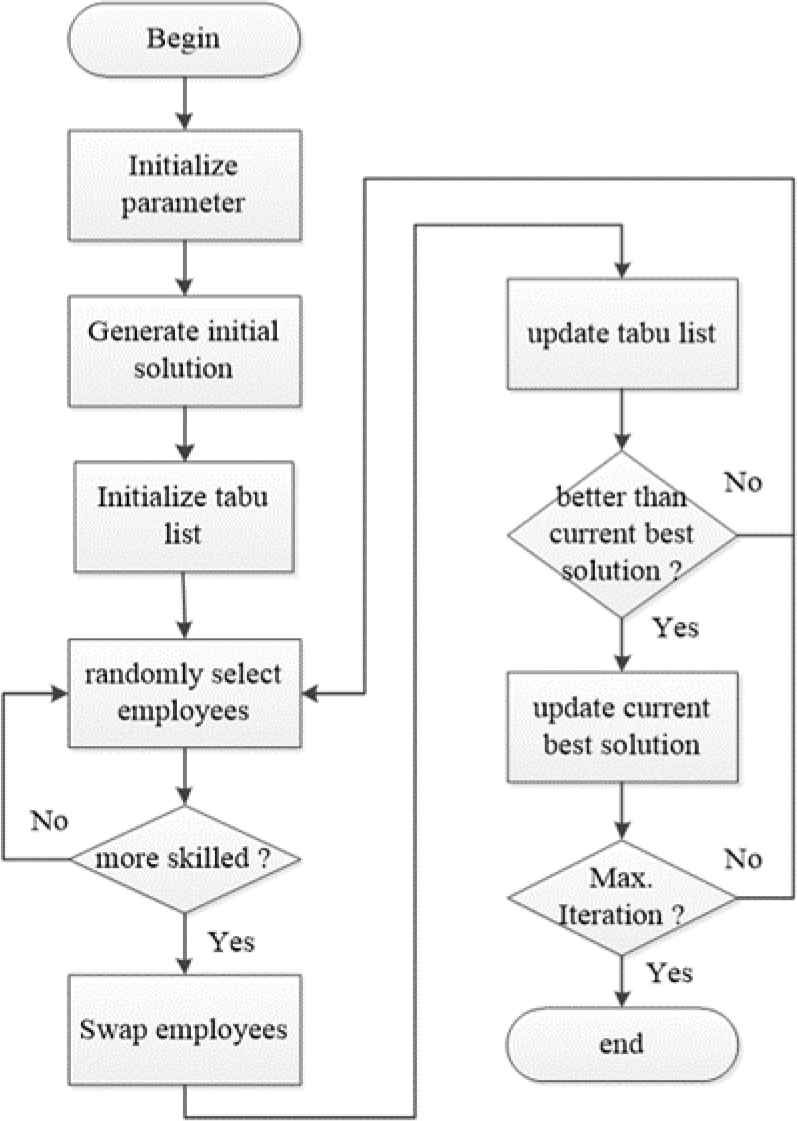
Tabu search for assembly line balancing problem with workers’ assignment.
3.5.3. SA steps
SA is a meta-heuristic, which imitates the annealing process in metallurgy by starting with the initial high temperature and slowly cooling down coupled with the Metroplis random sampling. The aim of the SA is to discover the global near-optimal solution. The algorithmic steps of SA are described as following and shown as Figure 6.
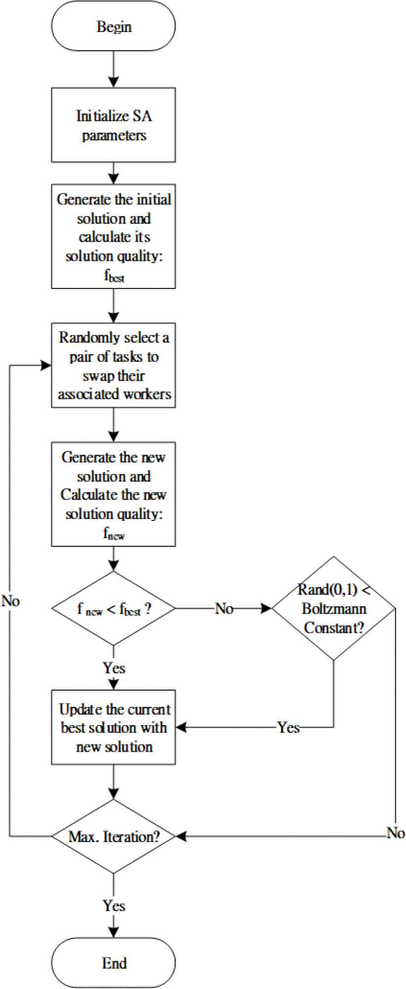
Simulated annealing for assembly line balancing with worker’s assignment.
Step 1. Similar to TS algorithm aforementioned, the workers are randomly assigned to tasks, and the adjusted processing time of each worker at each task is computed with respect to each individual’s skill proficiency.
Step 2. We Initialize the SA parameters: λ and T0. λ corresponds to the proportion of lowering the temperature while T0 corresponds to the initial temperature.
Step 3. We generate the initial solution, which is assigned as the current best solution, fbest, and calculate the solution’s fitness value or quality.
Step 4. We randomly select a pair of tasks for exchanging their corresponding workers.
Step 5. After the exchange, the new solution is generated and calculated its fitness or solution quality.
Step 6. Check the new solution, fnew, is less than the current best solution, fbest. If this is the case, the current best solution is updated with the new solution; otherwise, a random float number between (0, 1) is generated and compared against the Boltzmann constant. If the random value is less than the Boltzmann constant, the current best solution is updated with the new solution even though the new solution is no better than the current best solution. This type of update corresponds to the Metroplis random sampling strategy with the purpose to explore the global search.
Step 7. The algorithm is repeated until the maximum iteration is reached; in this case, the temperature has been lowered below the defined final temperature.
Step 8. Once the near-optimal solution of workers’ assignment to tasks is determined, the next step is to assign the tasks to the work stations with the restriction of not exceeding the average cycle time for every work station and following the precedence relationship.
4. RESULTS AND ANALYSIS
We would analyze and discuss the resulting outcomes of our proposed model in this section.
4.1. Research Environment
The research environments are as the following.
We wrote the algorithms in Java.
We executed the simulation under the Eclipse integrated development environment.
The PC where the simulation occurred consists of Intel (R) Core (TM) i3 CPU 2GB RAM PC.
4.2. Experiments and Data Analysis
Chan et al. [2] discuss the issues of task planning and personnel’s skill proficiency for men’s short-sleeved T-shirt production in the garment industry. In that paper, each task is associated with a standard allowable minute. However, Chan et al. [2] do not take into account of multitasking workers as introduced by the TPS. To better reflect the real-world scenario, thus we design two scenarios—single-task and multitask scenarios—where we assume that workers have arbitrary proficiencies at completing the tasks. The precedence relationship chart, the tables of 41-task processing time and workers’ skill tables according to Chan et al. [2] are provided as the following.
The precedence relationship of tasks is as shown in Figure 7 [13], which can be further identified as the task-work station assignment in Figure 8 [13]. During the simulations we do not update the task positions; however, we do adjust and decide the personnel assignment to tasks to obtain a better work cycle time.
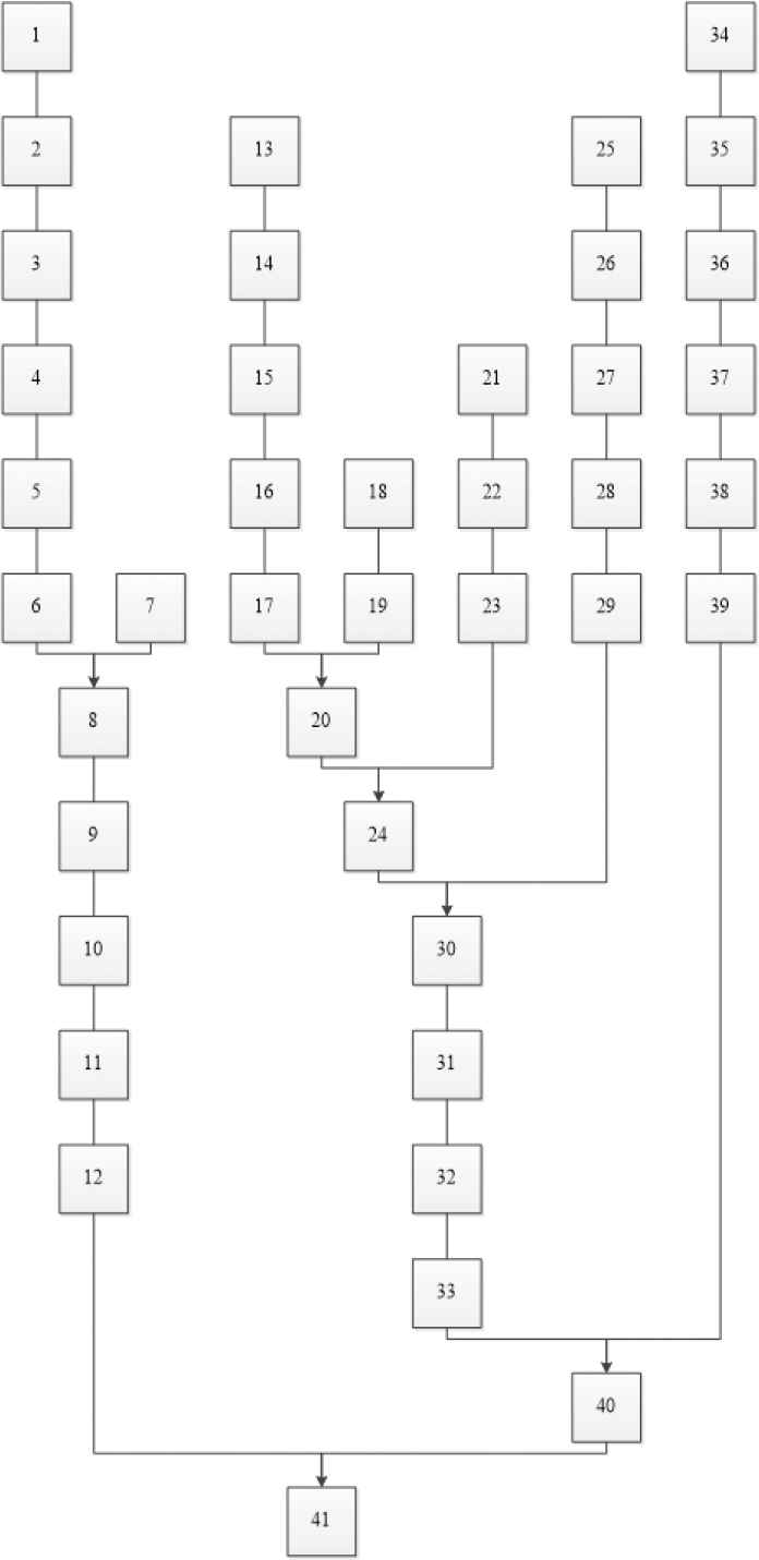
Task precedence relationship [13].
Lin [13] proposes the modular diagram by grouping tasks in the sub-assembly lines or branches of the precedence relationship [6] into modules or “work stations.” For example, Tasks 1–6 are grouped into a work station and so on. This configuration in Figure 7 is used in the simulations of multitasking workers later discussed.
The processing times of tasks in the garment industry are measured in standard allowable minutes, which consists of the basic time of the particular task and slack time (e.g., the allowable time of untying and tying garment bundles). By reducing the slack time, therefore, improve the standard allowable minutes [9]. Table 1 displays tasks and their corresponding standard allowable minutes.
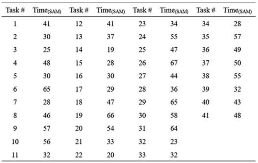 |
41-task and their processing time [2].
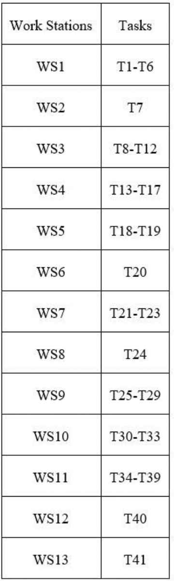
Task-work station assignment [13].
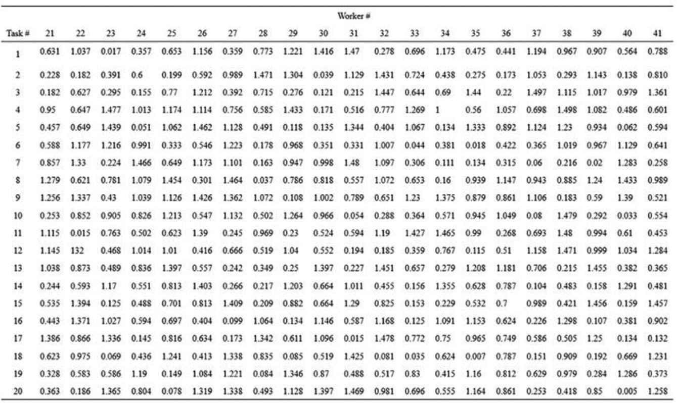
The workers’ performances for each task are rated from 0 (no skill at all) to 1.5 (fully skilled) according to the workers’ skill table provided by Chan et al. [2]. Due to the space limitation, we split up the 41-workers’ skill table into several sub-tables (Tables 2a–2d).
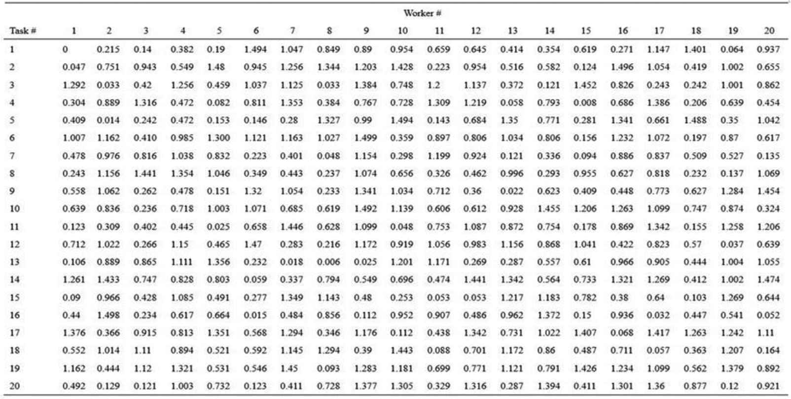 |
Worker skill (No. 1–20) vs. Task (No. 1–20) [2].
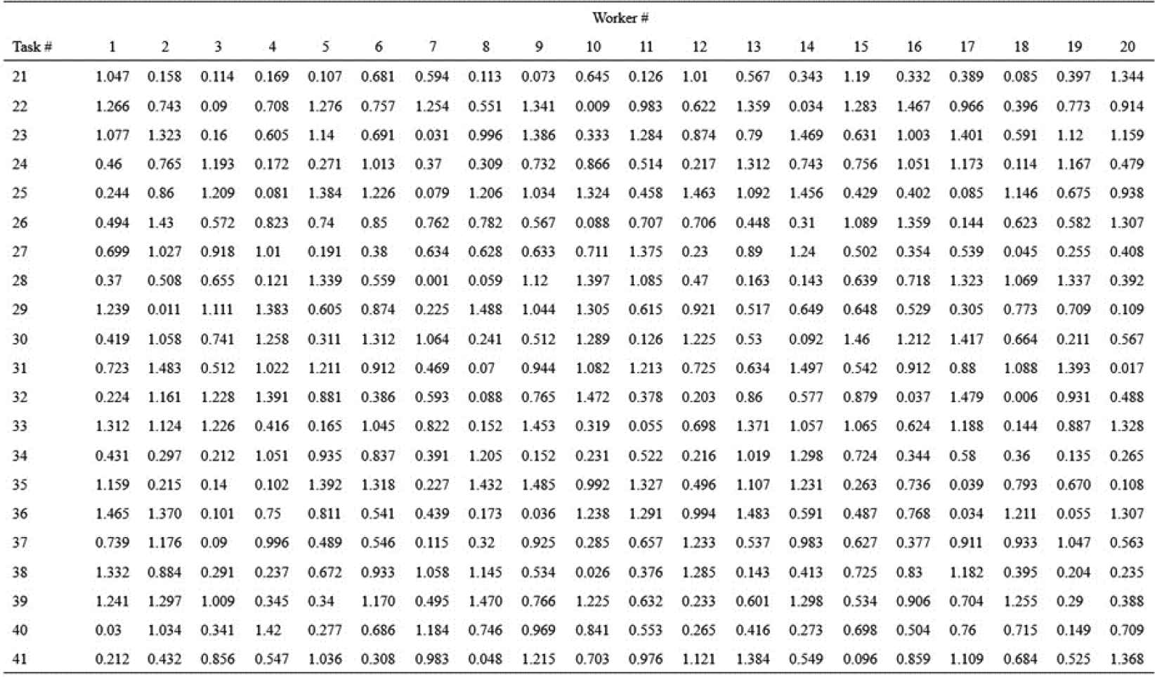 |
Worker skill (No. 1–20) vs. Task (No. 21–41) [2].
 |
Worker skill (No. 21–41) vs. Task (No. 1–20) [2].
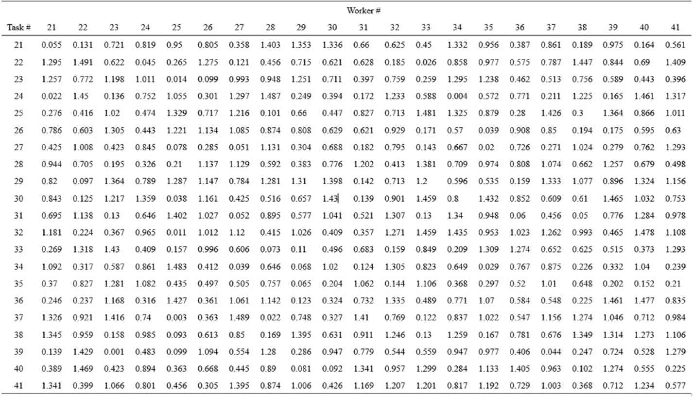 |
Worker skill (No. 21–41) vs. Task (No. 21–41) [2].
4.2.1. Worker’s assignment in the single-task mode
We first calculate the total processing time or standard allowable minutes of all tasks to be performed. In the example of the garment industry given by Chan et al. [2] the total processing time comes out to be 1,749 minutes. Next, we divide the total processing time by the number of work stations as indicated by the precedence relationship graph where each branch of the graph is an equivalent of a work station according to Chan et al. [2] and Lin [13]. The average processing time thus comes out to be roughly 135 minutes per work station. The calculated average processing time is used as the soft time constraint for assigning tasks to work stations to achieve the work balance. However, if the processing times of some tasks go slightly above the average processing time, the solution is still acceptable.
Table 3a provides the statistics on the CG algorithm and 13 work stations (corresponding to 13 branches) with task-worker assignments. The total adjusted SAM corresponding to the adjusted standard allowable minutes obtained from formula (5). The min and max correspond to the minimum and maximum work station processing times, respectively. The Std. Dev. represents the standard deviation of all the work station processing times. Additionally, Txx-Wxx represents the task and assigned worker numbers.
| Total adjusted SAM | 1,282.26 minutes | |
|---|---|---|
| Work station processing time statistics | Mean: 98.635; Min: 18.919; Max: 235.258; Std. Dev.: 69.964 | |
| Work station assignment | WS1 | {T1-W6, T2-W16, T3-W37, T4-W38, T5-W10, T6-W9} |
| WS2 | {T7-W31} | |
| WS3 | {T8-W27, T9-W20, T10-W14, T11-W34, T12-W22} | |
| WS4 | {T13-W39, T14-W12, T15-W41, T16-W2, T17-W32} | |
| WS5 | {T18-W8, T19-W7} | |
| WS6 | {T20-W30} | |
| WS7 | {T21-W28, T22-W13, T23-W17} | |
| WS8 | {T24-W40} | |
| WS9 | {T25-W33, T26-W23, T27-W11, T28-W5, T29-W4} | |
| WS10 | {T30-W15, T31-W25, T32-W3, T33-W1} | |
| WS11 | {T34-W21, T35-W24, T36-W18, T37-W19, T38-W29, T39-W26} | |
| WS12 | {T40-W36} | |
| WS13 | {T41-W35} | |
Statistics of constructive greedy algorithm for 13 work stations.
Furthermore, we also explore the possibility of assigning tasks to work stations based on the average processing time for the CG algorithm; that is, the accumulated processing time of tasks at a particular work station is less than the average processing time. Table 3b indicates the statistics of the work station processing time.
| Total adjusted SAM | 1,282.26 minutes | |
|---|---|---|
| Work station processing time statistics | Mean: 116.5689; Min: 93.649; Max: 132.904; Std. Dev: 14.73408 | |
| Work station assignment | WS1 | {T1-W6, T2-W16, T3-W37, T4-W38, T5-W10} |
| WS2 | {T6-W9, T7-W31, T8-W27, T9-W20} | |
| WS3 | {T10-W14, T11-W34, T12-W22, T13-W39, T14-W12} | |
| WS4 | {T15-W41, T16-W2, T17-W32, T18-W8} | |
| WS5 | {T19-W7, T20-W30, T21-W28, T22-W13} | |
| WS6 | {T23-W17, T24-W40, T25-W33} | |
| WS7 | {T26-W23, T27-W11, T28-W5} | |
| WS8 | {T29-W4, T30-W15, T31-W25} | |
| WS9 | {T32-W3, T33-W1, T34-W21, T35-W24} | |
| WS10 | {T36-W18, T37-W19, T38-W29} | |
| WS11 | {T39-W26, T40-W36, T41-W35} | |
Statistics of constructive greedy algorithm for nonpredetermined work stations.
In Table 4, the parameter values used in the TS are presented. The values are determined through the empirical approach. The number of iterations is user-defined at 1000 iterations; the length of Tabu list is set at 1681, which corresponds to number of workers × number of workers; the Tabu move is set at 5—number of iterations or time period within which the same move recorded in the Tabu list are prevented from making.
| Number of Iterations | Tabu List | Tabu Move |
|---|---|---|
| 1000 | 1681 | 5 |
Parameter values for Tabu search.
In Table 5, the parameter values of SA are presented. Three parameters are selected: the maximum iteration, λ (the proportional temperature cooling schedule) and initial temperature.
| Maximum Iteration | λ | Initial Temperature |
|---|---|---|
| 1000 | 0.70 | 100 |
Parameters for simulated annealing.
The results of TS executed for single-task workers are given in Table 6. Note that 24 work stations are required in this instance; the cycle time comes out to be 132 minutes.
| Total adjusted SAM | 2,325.415 minutes | |
|---|---|---|
| Work station processing time statistics | Mean: 96.892; Min: 47.235; Max: 131.998; std. Dev: 23.085 | |
| Work station assignment | WS1 | {T1-W25, T2-W6, T3-W39} |
| WS2 | {T4-W21, T5-W8} | |
| WS3 | {T6-W38, T7-W22} | |
| WS4 | {T8-W17, T9-W28} | |
| WS5 | {T10-W27} | |
| WS6 | {T11-W2} | |
| WS7 | {T12-W14} | |
| WS8 | {T13-W40, T14-W16, T15-W7} | |
| WS9 | {T16-W5, T17-W4, T18-W3} | |
| WS10 | {T19-W24, T20-W35} | |
| WS11 | {T21-W10, T22-W37} | |
| WS12 | {T23-W41} | |
| WS13 | {T24-W33} | |
| WS14 | {T25-W26, T26-W23} | |
| WS15 | {T27-W34} | |
| WS16 | {T28-W29} | |
| WS17 | {T29-W15} | |
| WS18 | {T30-W13} | |
| WS19 | {T31-W19, T32-W20} | |
| WS20 | {T33-W30, T34-W1} | |
| WS21 | {T35-W12} | |
| WS22 | {T36-W18, T37-W9} | |
| WS23 | {T38-W36, T39-W11} | |
| WS24 | {T40-W32, T41-W31} | |
Statistics of Tabu search for single-task workers for nonpredetermined work stations.
The results of SA executed for single-task workers are given in Table 7. Note that 21 work stations are required in this instance; the maximum cycle time comes out to be 183 minutes.
| Total adjusted SAM | 2,129.846 minutes | |
|---|---|---|
| Work station processing time statistics | Min: 47.714; Max: 183.007; Std Dev: 31.796 | |
| Work station assignment | WS1 | {T1-W18, T2-W37, T3-W38} |
| WS2 | {T4-W40} | |
| WS3 | {T5-W12, T6-W5, T7-W2} | |
| WS4 | {T8-W41, T9-W24} | |
| WS5 | {T10-W30, T11-W20, T12-W4} | |
| WS6 | {T13-W19, T14-W25} | |
| WS7 | {T15-W33} | |
| WS8 | {T16-W16, T17-W28} | |
| WS9 | {T18-W9} | |
| WS10 | {T19-W6} | |
| WS11 | {T20-W27, T21-W1, T22-W15} | |
| WS12 | {T23-W36, T24-W32} | |
| WS13 | {T25-W35} | |
| WS14 | {T26-W3} | |
| WS15 | {T27-W22, T28-W21} | |
| WS16 | {T29-W34} | |
| WS17 | {T30-W7, T31-W26} | |
| WS18 | {T32-W13, T33-W23, T34-W14, T35-W10} | |
| WS19 | {T36-W11, T37-W17} | |
| WS20 | {T38-W31, T39-W8, T40-W39} | |
| WS21 | {T41-W29} | |
Statistics of simulated annealing for single-task workers.
In the single-task worker scenario, we apply the CG algorithm, TS and SA algorithms to find solutions. The results indicate that in the single-task worker scenario, the CG algorithm for non-predetermined work stations performs the best among all the algorithms with shortest maximum cycle time and less work stations. The best solutions are obtained after 10 execution runs. Table 8 presents the comparison results of all algorithms executed in this paper.
| Fixed Size (CG)* | CG | TS | SA | |
|---|---|---|---|---|
| Best Soln. (maximum cycle time) | 235.258 | 132.904 | 131.998 | 183.007 |
| Number of work stations | 13 | 11 | 24 | 21 |
13 pre-determined work stations.
Comparison of solution results in the single-task scenario.
4.2.2. Worker’s assignment in the multitask scenario
In this section, we adopt the idea of TSS and make 30% of workers operate through multitasking approach (one staff being assigned to multiple tasks). Assume that we have 41 tasks and thus we will have 13 multitasking workstations. The configuration of task and work stations are shown earlier in Figure 7. Assigning one individual worker to a work station is an unique challenging problem since a worker has a portfolio of various skill levels for different tasks.
The CG algorithm operates on the principle of finding the “most fit” worker for a particular task. This principle works well for a single task; however, for a work station with multiple tasks assigned with a single worker, the strategy fails to produce promising results. This is understandable for a worker with wildly fluctuating skill levels for different tasks. Table 9 presents this point. The processing time of 13 work stations varies wildly from minimum of 18.919 minutes to maximum of 6124.305 minutes. On the other hand, with their improving and probabilistic nature of TS and SA in the multitasking mode understandably perform better by rejecting inferior solutions and keeping promising ones.
| Work station processing time statistics | Mean: 965.792; Min: 18.919; Max: 6124.305; Std Dev: 1861.080 | |
|---|---|---|
| Work station assignment | WS1 | {T[1-6]-W9} |
| WS2 | {T7-W31} | |
| WS3 | {T[8-12]-W20} | |
| WS4 | {T[13-17]-W39} | |
| WS5 | {T[18-19]-W7} | |
| WS6 | {T20-W30} | |
| WS7 | {T[21-23]-W14} | |
| WS8 | {T24-W28} | |
| WS9 | {T[25-29]-W2} | |
| WS10 | {T[30-33]-W25} | |
| WS11 | {T[34-39]-W8} | |
| WS12 | {T40-W22} | |
| WS13 | {T41-W27} | |
Statistics of constructive greedy algorithm for multitasking.
Table 10 shows the statistics of work station processing time and task-worker assignment for the TS. The processing time of 13 work stations for TS varies from minimum of 605.017 minutes to maximum of 2769.603 minutes.
| Work station processing time statistics | Mean: 605.017; Min: 91.503; Max: 2769.603; Std Dev: 755.573 | |
|---|---|---|
| Work station assignment | WS1 | {T[1-6]-W12} |
| WS2 | {T7-W33} | |
| WS3 | {T[8-12]-W13} | |
| WS4 | {T[13-17]-W11} | |
| WS5 | {T[18-19]-W28} | |
| WS6 | {T20-W15} | |
| WS7 | {T[21-23]-W6} | |
| WS8 | {T24-W7} | |
| WS9 | {T[25-29]-W29} | |
| WS10 | {T[30-33]-W10} | |
| WS11 | {T[34-39]-W2} | |
| WS12 | {T40-W1} | |
| WS13 | {T41-W26} | |
Statistics of tabu search for multitasking.
Table 11 shows the statistics of work station processing time and task-worker assignment for the SA search. The processing time of 13 work stations for SA varies from minimum of 762.782 minutes to maximum of 4129.875 minutes.
| Work station processing time statistics | Mean: 762.782; Min: 38.654; Max: 4129.875; Std Dev: 1211.692 | |
|---|---|---|
| Work station assignment | WS1 | {T[1-6]-W3} |
| WS2 | {T7-W6} | |
| WS3 | {T[8-12]-W25} | |
| WS4 | {T[13-17]-W33} | |
| WS5 | {T[18-19]-W8} | |
| WS6 | {T20-W30} | |
| WS7 | {T[21-23]-W2} | |
| WS8 | {T24-W16} | |
| WS9 | {T[25-29]-W35} | |
| WS10 | {T[30-33]-W21} | |
| WS11 | {T[34-39]-W10} | |
| WS12 | {T40-W11} | |
| WS13 | {T41-W4} | |
Statistics of simulated annealing for multitasking.
The following Table 12, displays the statistics of execution results by three algorithms. The results indicate that the TS is the best among those three when it comes to multitasking. The reason behind this may be the random skills of workers make it harder to apply greedy approach of assigning a particular best worker to a particular work station since no worker has the best of all skills (skills are varied) for a particular work station. Since the TS and SA are both improvement algorithms, they fares better than the CG algorithm which operates only on finding the best worker for a single task. Nevertheless, because a single worker may not perform top-notched for all tasks for a work station with multiple tasks, the processing time suffers for the CG algorithm.
| CG | TS | SA | |
|---|---|---|---|
| Best Soln. (maximum cycle time) | 6124.305 | 2769.603 | 4129.875 |
Best solutions of three algorithms for multitasking.
4.2.3. Discussion
In this section, we summarize and compare our research analysis. As mentioned earlier, there are few studies investigating into the issue of “labor skill”— a resource assignment problem with task precedence. This encourages us to adopt the concept of the labor skill in our model and further apply meta-heuristic algorithms to solve for the optimal solutions. With the data from Chan et al. [2], we executed the single-tasking and multitasking experiments against the CG algorithm, TS algorithm and SA approach. In the single-task scenario, the CG method turns out to be the best approach, with less required number of work stations and lowest cycle time. On the other hand, the TS outperforms both CG algorithm and SA in terms of the lowest maximum cycle time of the entire assembly line. It is worthy of mentioning that our research utilizes the existing meta-heuristic algorithms to derive the near-optimal solutions within a limited time. This would assist garment industry in implementing the scheduling model with consideration of the labor skill in an efficient manner. Furthermore, because of the Internet of Things (IoT) trend, one can expect that the data at the shop floor can be automatically collected. We can apply the labor performance data captured by tasks and then employ the artificial intelligence (AI) model to predict the behaviors of labors. This would be more accurate to formulate the labor skills in our model.
5. CONCLUSIONS AND RECOMMENDATIONS
In this research, we apply the TS and SA algorithms to solve the ALB problem considering the labor-intensive nature of the garment industry. The objective of the proposed model is to minimize the cycle time in the assembly line performed through task placement. Nevertheless, in the garment industry, since tasks or machines usually are placed at fixed positions at the early stage of facility layout planning, the cycle time can be minimized via the staff assignment. Based on the resulting outcomes for the single-task scenario, the CG method outperforms TS and SA in two aspects: work stations numbers and cycle time. Furthermore, this paper also adopts the multitasking concept of TSS derived from TPS to solve the ALB problem in the garment industry by assigning 30% of workers to work stations in the multitasking mode. The TS comes out to be the winner in terms of the lowest cycle time. We observe that with a worker with randomized skill levels for different tasks as given by [6], it is less likely that a worker, exceptional for a single task, may perform equally well against multiple tasks. Therefore, in regards to the managerial implication, a team of workers with specific talents (high skill proficiency) for particular tasks performs better than multitasking workers with disparate skill levels do.
We outline the contributions of this research as following.
Three algorithms—CG, TS and SA algorithms—are proposed and discussed.
The original single-task mode of production line is revised; 30% labor force are assigned to work stations in the multitasking scenario.
In our research, we adjust the cycle time based on employee’s proficiency assignment to calculate the cycle time. To reflect the reality of the world, we consider employee’s skill to update the standard task working time. Although, TSS promote the concept of multitasking, it should be noted that the existing limitations of production processes prevent the entire update of all or most single production into multitasking mode. For example, the turnover rate of skilled or cross-trained workers can be quite high. This may discourage employers from cross-training the entire workforce. Additionally, the ramp-up time for multitasking may dissuade the management to put new workers immediately in a cell to handle multiple tasks. Therefore, in our research we only consider 30% of workforce as multitasking workers in terms of predetermined number of work stations. For future work, we suggest a number of issues for future researchers.
Our research focuses on the scenario of tasks placed at fixed positions at the construction stage—we can only change labor assignment. For further investigation, we may take into consideration of both employee and task swapping.
In the research, we implement CG, TS and SA algorithms in this research. We can employ other approaches in the future research.
The study is concerned with a single objective—the cycle time; multiple objectives may be investigated in the future.
Due to the trend of IoT and applications of AI, researchers may further incorporate the machine learning algorithms into our model to better predict the performance of labor.
AUTHORS' CONTRIBUTIONS
Gary Yu-Hsin Chen: Conceptualization, Software, Investigation, Writing - Original Draft, Funding acquisition. Ping-Shun Chen: Methodology, Supervision, Software. Jr-Fong Dang: Formal analysis, Writing - Review & Editing, Project administration. Sung-Lien Kang: Investigation, Resources. Li-Jen Cheng: Software, Writing - Original Draft.
ACKNOWLEDGMENTS
This work was supported by Ministry of Science and Technology of Taiwan under Grant MOST 108-2221-E-992-019-.
REFERENCES
Cite this article
TY  - JOUR
AU  - Gary Yu-Hsin Chen
AU  - Ping-Shun Chen
AU  - Jr-Fong Dang
AU  - Sung-Lien Kang
AU  - Li-Jen Cheng
PY  - 2021
DA  - 2021/04/26
TI  - Applying Meta-Heuristics Algorithm to Solve Assembly Line Balancing Problem with Labor Skill Level in Garment Industry
JO  - International Journal of Computational Intelligence Systems
SP  - 1438
EP  - 1450
VL  - 14
IS  - 1
SN  - 1875-6883
UR  - https://doi.org/10.2991/ijcis.d.210420.002
DO  - 10.2991/ijcis.d.210420.002
ID  - Chen2021
ER  -