
Improved Knowledge Measures for q-Rung Orthopair Fuzzy Sets
- DOI
- 10.2991/ijcis.d.210531.002How to use a DOI?
- Keywords
- Knowledge measure; q-rung orthopair fuzzy sets; Entropy; MAGDM
- Abstract
The q-rung orthopair fuzzy set (qROFS) defined by Yager is a generalization of Atanassov intuitionistic fuzzy set (IFS) and Pythagorean fuzzy sets (PyFSs). In this paper, we define the knowledge measure for qROFS by using the cosine inverse function. The information precision and information content are two facets of knowledge measure. Both facets of knowledge measure are considered. The properties of knowledge measure and their graphical explanations are discussed. An application of the knowledge measure in multi-attribute group decision-making (MAGDM) problem under the confidence level approach is given. A numerical example of the selection of renewable energy sources is discussed.
- Copyright
- © 2021 The Authors. Published by Atlantis Press B.V.
- Open Access
- This is an open access article distributed under the CC BY-NC 4.0 license (http://creativecommons.org/licenses/by-nc/4.0/).
1. INTRODUCTION
The membership function is employed to represent the information in the fuzzy sets theory [1]. Real-world hesitations can be handled impressively by fuzzy set theory. Atanassov explicated intuitionistic fuzzy set (IFS) as a generalization of the fuzzy set theory [2]. The information in IFS is portrayed in the form of membership (favor) and nonmembership (against) functions. The membership and nonmembership degrees allocate the values from the unit interval [0,1] with the constraint that their sum is less than or equal to one that is if we represent the associate (membership) and nonassociate (nonmembership) functions by
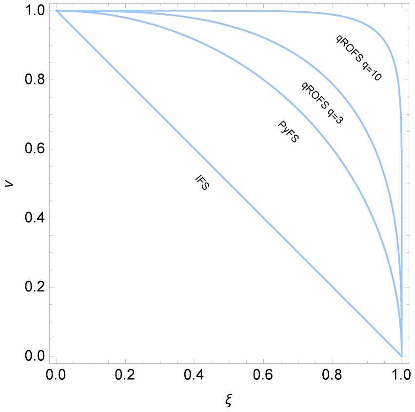
Graphical representation of IFS, PyFS and qROFSs (q = 3,10).
Yager defined Pythagorean fuzzy set (PyFS) as a generalization of IFSs and extends the range of membership and nonmembership functions that is decision-makers express their judgments more freely than IFSs [3,4]. The membership
Yager introduced the concept of q-rung orthopair fuzzy set (qROFS) as a generalization of both IFSs and PyFSs [9,10]. The condition for the membership
Figure 1 differentiate the set of order pairs available for membership and nonmembership grades for IFSs, PyFSS and qROFSs (or margin for decision-makers to make their judgments). According to Ali [11], the range of the membership functions in IFS has an area 0.5 square unit in Figure 1. For PyFS the area increases to 0.77854 square unit which is 57% more than from the IFS case. For qROFS (q=3), the area increases to 0.8832, which is approximately 13% more than the PyFS case. The range of the membership function covers up to 99% region of the unit square [0,1] × [0,1] for q=10 (see Figure 1). So for real-life applications, the value of q up to 10 is more suitable although q is the real number.
The notion of neutrosophic sets is quite different from qROFSs. In neutrosophic sets
While dealing with real-life situations qROFSs provide more flexible ways to define membership and non-membership grades. That is why nowadays many researchers are showing keen interest in qROFSs. Hussain et al. [13] combined the qROFS with soft sets and defined their aggregation operators. The generalized Maclaurin symmetric mean operators, the exponential aggregation operators, the aggregation operators, the interaction Hamy mean operators, the Dombi power partitioned Heronian mean operators, the power Maclaurin symmetric mean operators, the Heronian mean operators and the power aggregation operators for qROFSs were expounded in [14–20], respectively. The multiple heterogeneous relationships between membership functions and criterion were explored by Yang et al. [21]. Verma [22] explained order-
De Luca and Termini [34] introduced the axioms for fuzzy entropy which measures the fuzziness for fuzzy sets. Entropy has been a rich area of interest for many researchers. Entropy for IFSs was expounded by Bustince and Burillo [35]. Later Szmidt and Kacprzyk [36] defined a ratio based entropy by using the Hamming distance. The information about an intuitionistic fuzzy value (IFV) is conveying properly by this entropy that is how much intuitionistic fuzzy is an IFV? The distance, similarity, entropy and inclusion measures for qROFSs were expounded by Peng and Liu [37].
The dissimilarity and similarity measures is a rich area for scholars. Keeping in mind the applications of this area many researchers work on dissimilarity and similarity measures. The applications of this area was discussed in medical diagnosis, data mining, pattern recognition, decision-making, clustering and in image processing. The qROF multi-parametric similarity measure and combinative distance-based assessment were used to assess the classroom teaching quality [38]. The dissimilarity, similarity, entropy and inclusion measures for qROFSs were defined by Peng and Liu [37]. The similarity measures of qROFSs based on cosine and cotangent functions were expounded by Wang et al. [39]. The Minkowski dissimilarity measures (Hamming, Euclidean and Chebyshev distances) for qROFSs were discussed in [40]. The TOPSIS method based on improved cosine similarity measures was interpreted in [41]. A new dissimilarity measure was defined with a nice interpretation. The TOPSIS and ELECTRE were described based on this novel dissimilarity measure for qROFSs in [42].
Knowledge is basically related to the information considered in a particular useful context. The amount of information and the amount of knowledge are closely linked. From practical point of view, the transformation of information into the knowledge is very important, like in decision-making. Generally it is thought that knowledge measure is the dual of the entropy [43]. This approach is also adopted in [44,45]. In this regard the point of view given by Szmidt et al. [46] is bit different and they consider that a knowledge measure must depend on both hesitancy index and the entropy. Therefore while defining a knowledge measure in IFSs, both uncertainty index and entropy must be taken into account [46]. So a knowledge measure for IFSs is given in [46], which is based on both uncertainty index and entropy. It was expected that for a constant value of uncertainty index the knowledge measure defined in [46] must behave dually to entropy. Actually this does not happen for the above mentioned knowledge measure. Guo [47] and Guo and Xu [48] think that the entropy and knowledge are two distinct measures therefore these should be dealt independently. An axiomatic definition of knowledge measures is given in [47,48]. Knowledge measure in [48] is based on information clarity and information content. Singh et al. [49] proposed the knowledge, entropy and inclusion measures for fuzzy sets and it’s application in image processing. For more literature on knowledge measure, refer to [50,51].
In the first approach, the axiomatic framework of knowledge measures for qROFSs was defined [52]. The previous approach has considered the hesitancy index only. The higher value of knowledge measure is attached to qROFS with lower hesitancy indices. In other words, the approach considers the information content that is the maximum information content that results in the maximum knowledge measure. But the approach not considered the information clarity or information precision. So, the proposed approach contemplate the both aspect of knowledge measure that is the information content and information precision.
Since the qROFS is a generalization of both IFSs and PyFSs. Thus the existing models to quantify the knowledge from the intuitionistic fuzzy information are not suitable for Pythagorean and q-rung orthopair fuzzy environment. Therefore, we need to define a new generalized knowledge measure for q-rung orthopair fuzzy environment that quantifies the information from qROFSs.
Motivated by the Yager approach, we propose a method to quantify the knowledge associated with qROFS. The knowledge associated with q-rung orthopair fuzzy values (qROFVs) increases for assured and precise information and decreases when the ambiguity and uncertainty factor increases. The knowledge measure also depend both on information precision and information content. Also, the confidence level approach towards MAGDM problems is essential in the information fusion step. But there does not exist any study about how to find the confidence level. We have formulated a procedure to find the confidence level in the information fusion step.
To measure the amount of knowledge from information provided in the form of qROFS, a novel axiomatic framework is proposed in this paper that consider the information precision and information content. The main contributions of our work are:
A knowledge measure for qROFS based on inverse cosine function is defined.
The axiomatic characterization results are obtained for the proposed knowledge measure.
Properties of knowledge measure with their graphical representation are discussed.
A method to solve MAGDM problems under confidence level is proposed.
The proposed knowledge measure differentiates among the two clearly different situations: (i) the membership and non-membership functions both have same values (i.e., we have equal number of arguments in favor and against). (ii) We have no information at all (i.e., the membership and nonmembership functions both have values zero).
The remaining part of the paper is designed as follows: Section 2 consists of the basic definitions related to the IFS, PyFS and qROFS. An axiomatic definition of knowledge measure and its related properties with graphical explanations are investigated in Sections 3–5. The applications of the proposed knowledge measure in MAGDM problems under confidence level approach are explored in Section 6. The summary, limitations and future directions are debated in Section 8.
2. PRELIMINARIES
In this segment, the definitions of IFS, PyFS and qROFS and their properties are mentioned. Let X = {t1,t2,…,tn} represents the universal set throughout the paper which is discrete, finite and nonvoid discourse set. The membership and nonmembership functions and unit interval [0,1] are represented as
Definition 1.
An IFS R on a universal set X is defined as
Definition 2.
[3,4] A PyFS R on a universal set X is defined as
Definition 3.
[9,10] A qROFS R on a universal set X is defined as
For any two qROFVs
3. KNOWLEDGE MEASURE
Knowledge is basically related to the information considered in a particular useful context. The amount of information and the amount of knowledge are closely linked. From practical point of view, the transformation of information into the knowledge is very important, like in decision-making. In this part, we define the knowledge measure for qROFS by using the cosine inverse function. The information precision and information content are two facets of knowledge measure. Both facets of knowledge measure are consider in the given method.
In the following, we provide the axiomatic definition of knowledge measure for qROFSs.
Definition 4.
The knowledge measure
K1.
K2.
K3.
K4.
Now, we define the knowledge measure for qROFS by using cosine inverse function. The knowledge is measured by considering membership, nonmembership and hesitancy degrees.
Definition 5.
Let R be a qROFS in X. Then, the knowledge measure of R is defined and expressed as
Since
If X = {t}, then the knowledge measure for a qROFS R is represented as
Remark 1.
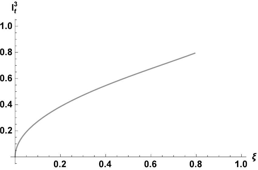
It is important to note that the knowledge measure presented in Equation (3) has two parts, that is,
Since there is maximum opacity at
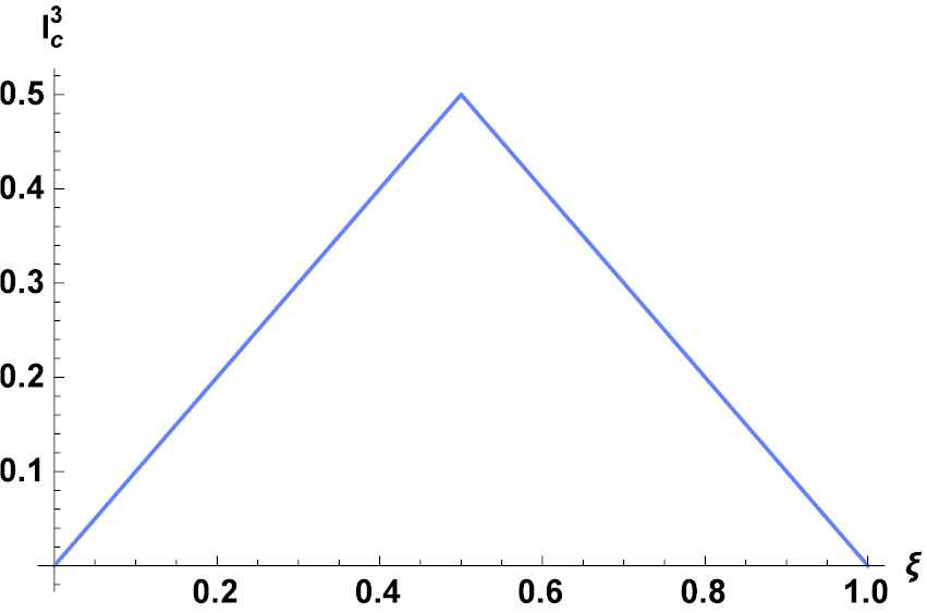
The information content is maximum at
The graphical representation of both parts displaced in Figures 2 and 3. It can easily be seen from Figure 2 that the first part have value one two times for crisp cases and remains zero for
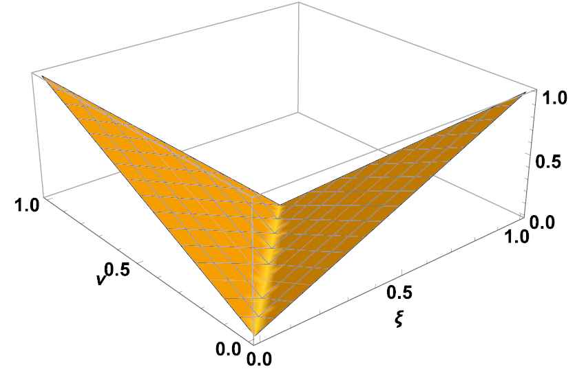
First part of Equation (3).
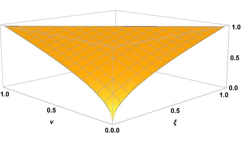
Second part of Equation (3).
The following axiomatic properties are satisfied for the proposed knowledge measure
Theorem 1.
If
(K1).
(K2).
(K3).
(K4).
Proof.
Proof. (K1). Since
The left-hand side of the Equation (4) has two parts, that is,
Thus Equation (4) holds only when both parts have value one, that is,
Now,
Therefore, the necessary and sufficient condition for Equation (4) to hold is
Hence it holds only for crisp sets.
(K2). From Equation (2), we have
The left-hand side of the Equation (6) has two parts, that is,
Now,
Therefore, the necessary and sufficient condition for Equation (6) to hold is
(K3). To prove the axiom
To complete the proof, we need to show the function in Equation (8) monotonically increasing with respect to
So, the Equations (9) and (10) show the required monotonicity.
4. PROPERTIES OF KNOWLEDGE MEASURE I c q
This part consist of properties and analysis of the knowledge measure
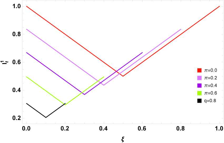
P1: Figure 4 shows the geometric interpretation of knowledge measure
Point
While points
The graph remains symmetric around line
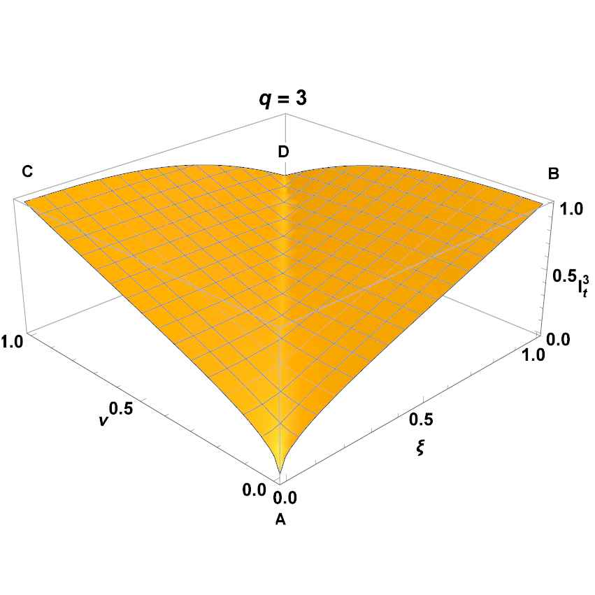
Graphical representations of knowledge measure
P2: The proposed knowledge measure
The membership
We have no information at all (the membership and nonmembership functions have values zero, i.e.,
In fact, the information measure should be different for the most fuzzy qROFS
Equation (11) shows that there is no information precision for
Figure 5 shows the geometric interpretation of knowledge measure
Knowledge measure when
P3: Now we consider the case when
Since the information content is maximum at
P4: The proposed knowledge measure
As a dual measure, the entropy measure of fuzzy set
The geometric interpretation of E(R) is given in Figure 6. From Figure 6, we can easily see that E(R) has value zero only for crisp cases. E(R) has maximum value at (x,0.5,0.5). At last, E(R) is greater than E(S) where R is any “sharpened" version of
Knowledge measure as De Luka and Termini entropy.
P5: Next, we have seen that when π(t)=c (constant), then
Now, the part
Definition 6.
To make analysis more clear and understandable, for each fixed value of
Remark 2.
For each fixed value of
Theorem 2.
The relation
Proof.
Straightforward
From Theorem 2, it is clear that the quotient set is defined with the help of
It is important to note that for each class
The shape of some classes generated by relation
It is necessary to observe the behavior of the classes in
5. ENTROPY INDEPENDENT KNOWLEDGE MEASURE
In this section, the analytical and numerical proofs are provided to prop the entropy independent knowledge measure. Entropy for qROFSs was defined by Peng and Liu [37] and discussed twelve different models that fulfilled the required properties for entropy measure. To discuss the relation between knowledge and entropy measures for qROFSs, let us recall the axioms for entropy measure presented in [37].
Definition 7.
The entropy measure
E1.
E2.
E3.
E4.
Axioms E1 and E4 in Definition 5 are closely related to the axioms K1 and K4 in Definition 3. The Axioms E2 and K2 are significantly different from each other, like if we consider the knowledge measure as a dual of entropy then it attains value one whenever
Now, the conditions in axiom
On the other hand if
6. APPLICATION IN MCGDM PROBLEMS
This section is devoted to the application of knowledge measure in MCGDM problems. The confidence q-rung orthopair fuzzy Einstein weighted averaging (CqREWA) operator, decision-making process, CRITIC method are discussed in this section. At the end, a step-wise procedure for MCGDM problems is discussed.
6.1. q-Rung Orthopair Fuzzy Einstein-Weighted Averaging Operator Under Confidence Level
Besides these achievements under the generalizations of a fuzzy environment, few existing approaches consolidate the familiarity degree in the information fusion step. The specialist in an MCDM problem assesses the alternatives based on the mentioned criteria only, that is, the familiarity (called confidence levels) of the specialist with the evaluation objects is not incorporated in most of the existing studies. So, it is a must to include the familiarity of an expert in the original information. Xia et al. [53] formulated the induced aggregation operators for fuzzy and hesitant fuzzy sets. The aggregation operators under the confidence level for IFSs were considered by Yu [54]. Garg [55] expounded the confidence levels based on Pythagorean fuzzy aggregation operators. The qROF aggregation operators under confidence level were proposed by Joshi and Gegov [56].
Yu [54] and Rahman et al. [57] discussed the confidence intuitionistic fuzzy Einstein weighted averaging operators and generalized confidence intuitionistic fuzzy Einstein hybrid averaging/geometric operators, respectively. They discussed the closure property with respect to their environments. So, we will extend their approach to qROFSs and define CqREWA operator. Since, the operator CqREWA is a natural extension of them, so it definitely closed with respect to qROFSs. The details of the proposed aggregation operator and geometric and hybrid aggregation operators will be discuss in another paper.
Definition 8.
Let
6.2. Decision-Making Process
The aim of decision making process is to select the favorite alternative on the basis of the criteria defined by the experts. In decision-making process, let
| Linguistic Variables | Corr. qROFVs | Linguistic Variables | Corr. qROFVs |
|---|---|---|---|
| EH | (0.9, 0.1) | L | (0.4, 0.6) |
| VH | (0.8, 0.2) | VL | (0.25, 0.75) |
| H | (0.7, 0.3) | EL | (0.1, 0.9) |
| F | (0.5, 0.5) |
A linguistic ratings and their corresponding.
6.3. CRITIC Method
Diakoulaki et al. [58] have proposed the CRITIC (The Criteria Importance Through Intercriteria Correlation) method that uses correlation analysis to detect contrasts between criteria and standard deviation, which quantifies the contrast intensity of the corresponding criterion [59]. The method developed is based on the analytical investigation of the evaluation matrix for extracting all information contained in the evaluation criteria [59]. The CRITIC method reflects the inner information of data transmission and the approximation of subjective weight to some extent. Thus Yalcin and Unlu [60] used CRITIC method to obtain weights for IPO performance analysis, Tus and Adali [61] used for attendance software assessment, and Peng et al. [62] used to obtain weights for 5G industry evaluation.
The weights of criteria are formulated by CRITIC method by following steps:
Step 1: Calculate the knowledge measure
Step 2: Normalize the matrix
Step 3: The standard deviations for each criterion are calculated by Equation (21).
Step 4: Correlation coefficients between each criterion are calculated by Equation (22) which constitute the correlation coefficient matrix
Step 5: The quantity of information of each criterion are computed using standard deviation and correlation coefficient as follows:
Step 6 The weights of criteria are based on quantity of information and determine by Equation (24) as follows:
6.4. Proposed MCGDM Method
To understand the whole procedure of the MCGDM method, we divided into 6 steps.
Let
Step 2: Normalize the qROF decision matrix
Since the knowledge measure
Step 3: The information from qROF decision matrices
Step 4: Weights
Step 5: Again, the CqREWA operator is use to aggregate the information from qROF decision matrix
Step 6: Rank the qROFVs
6.5. Renewable Energy Source Selection by Proposed Method
The dependence on imported sources are very much reduced and the security of supply are provided by renewable energy (RE). RE addressed our energy needs by replacing foreign energy imports with reliable and clean home-grown electricity. Also, RE added bonus of fantastic local economic opportunities. By using RE instead of fossil fuels, we would significantly decrease the current levels of greenhouse gas emissions, and this would have positive environmental impact for our entire planet. RE is not all about environment as it can also give strong boost to our economy in form of new jobs. RE often referred to as clean energy, comes from natural sources or processes that are constantly replenished. For example, sunlight or wind keep shining and blowing, even if their availability depends on time and weather. Many studies have made to analyze and prioritize the RE sources for a region. These studies were based on some suitable MCGDM methods. Interested reader can find the relevant studies in [64,65]. We discuss here a general method to select and prioritize the RE source against the prescribed criteria.
Let
Step 1 & 2: Each individual decision maker
| e1 | e2 | e3 | e4 | e5 | e6 | e7 | e8 | e9 | e10 | e11 | e12 | |
|---|---|---|---|---|---|---|---|---|---|---|---|---|
| t1 | VH | F | H | EH | F | EH | VH | F | H | EL | F | EH |
| t2 | L | F | VH | H | EH | H | L | F | VH | H | EH | H |
| t3 | EH | L | F | VH | VL | VH | EH | L | F | VH | VL | VH |
| t4 | H | F | VH | L | H | F | H | F | VH | L | H | F |
| t5 | F | H | VH | VL | VH | F | F | H | VH | VL | VH | VL |
Performance comparison with state-of-the-art methods. The number in red indicates the best result and the number in blue indicates the second best result.
| e1 | e2 | e3 | e4 | e5 | e6 | e7 | e8 | e9 | e10 | e11 | e12 | |
|---|---|---|---|---|---|---|---|---|---|---|---|---|
| t1 | F | F | H | H | F | EH | VH | F | H | L | F | EH |
| t2 | EL | F | VH | H | H | H | L | F | VH | H | F | H |
| t3 | H | L | F | H | VL | VH | EH | L | F | H | VL | H |
| t4 | H | H | H | L | H | EH | H | F | VH | VL | H | F |
| t5 | H | L | VH | L | VH | F | F | H | VH | L | VH | VL |
Associated linguistic information by
| e1 | e2 | e3 | e4 | e5 | e6 | e7 | e8 | e9 | e10 | e11 | e12 | |
|---|---|---|---|---|---|---|---|---|---|---|---|---|
| t1 | VH | F | F | EH | F | H | VH | L | H | EL | F | H |
| t2 | H | F | H | H | EH | H | L | F | F | H | EH | H |
| t3 | H | F | F | VH | L | H | EH | L | F | VH | VL | VH |
| t4 | VH | F | H | L | H | F | H | F | VH | F | H | F |
| t5 | H | H | VH | L | VH | F | F | H | VH | VL | L | L |
Associated linguistic information by
| e1 | e2 | e3 | e4 | e5 | e6 | |
| t1 | ((0.8, 0.2), 0.84) | ((0.5, 0.5), 0.61) | ((0.7, 0.3), 0.76) | ((0.9, 0.1), 0.92) | ((0.5, 0.5), 0.61) | ((0.9, 0.1), 0.92) |
| t2 | ((0.4, 0.6), 0.68) | ((0.5, 0.5), 0.61) | ((0.8, 0.2), 0.84) | ((0.7, 0.3), 0.76) | ((0.9, 0.1), 0.92) | ((0.7, 0.3), 0.76) |
| t3 | ((0.9, 0.1), 0.92) | ((0.4, 0.6), 0.68) | ((0.5, 0.5), 0.61) | ((0.8, 0.2), 0.84) | ((0.25, 0.75), 0.80) | ((0.8, 0.2), 0.84) |
| t4 | ((0.7, 0.3), 0.76) | ((0.5, 0.5), 0.61) | ((0.8, 0.2), 0.84) | ((0.4, 0.6), 0.68) | ((0.7, 0.3), 0.76) | ((0.5, 0.5), 0.61) |
| t5 | ((0.5, 0.5), 0.61) | ((0.7, 0.3), 0.76) | ((0.8, 0.2), 0.84) | ((0.25, 0.75), 0.80) | ((0.8, 0.2), 0.84) | ((0.5, 0.5), 0.61) |
| e7 | e8 | e9 | e10 | e11 | e12 | |
| t1 | ((0.8, 0.2), 0.84) | ((0.5, 0.5), 0.61) | ((0.7, 0.3), 0.76) | ((0.1, 0.9), 0.92) | ((0.5, 0.5), 0.61) | ((0.9, 0.1), 0.92) |
| t2 | ((0.4, 0.6), 0.68) | ((0.5, 0.5), 0.61) | ((0.8, 0.2), 0.84) | ((0.7, 0.3), 0.76) | ((0.9, 0.1), 0.92) | ((0.7, 0.3), 0.76) |
| t3 | ((0.9, 0.1), 0.92) | ((0.4, 0.6), 0.68) | ((0.5, 0.5), 0.61) | ((0.8, 0.2), 0.84) | ((0.25, 0.75), 0.80) | ((0.8, 0.2), 0.84) |
| t4 | ((0.7, 0.3), 0.76) | ((0.5, 0.5), 0.61) | ((0.8, 0.2), 0.84) | ((0.4, 0.6), 0.68) | ((0.7, 0.3), 0.76) | ((0.5, 0.5), 0.61) |
| t5 | ((0.5, 0.5), 0.61) | ((0.7, 0.3), 0.76) | ((0.8, 0.2), 0.84) | ((0.25, 0.75), 0.80) | ((0.8, 0.2), 0.84) | ((0.25, 0.75), 0.80) |
Converted qROFVs information for
| e1 | e2 | e3 | e4 | e5 | e6 | |
| t1 | ((0.5, 0.5), 0.61) | ((0.5, 0.5), 0.61) | ((0.7, 0.3), 0.76) | ((0.7, 0.3), 0.76) | ((0.5, 0.5), 0.61) | ((0.9, 0.1), 0.92) |
| t2 | ((0.1, 0.9), 0.92) | ((0.5, 0.5), 0.61) | ((0.8, 0.2), 0.84) | ((0.7, 0.3), 0.76) | ((0.7, 0.3), 0.76) | ((0.7, 0.3), 0.76) |
| t3 | ((0.7, 0.3), 0.76) | ((0.4, 0.6), 0.68) | ((0.5, 0.5), 0.61) | ((0.7, 0.3), 0.76) | ((0.25, 0.75), 0.80) | ((0.8, 0.2), 0.84) |
| t4 | ((0.7, 0.3), 0.76) | ((0.7, 0.3), 0.76) | ((0.7, 0.3), 0.76) | ((0.4, 0.6), 0.68) | ((0.7, 0.3), 0.76) | ((0.9, 0.1), 0.92) |
| t5 | ((0.7, 0.3), 0.76) | ((0.4, 0.6), 0.68) | ((0.8, 0.2), 0.84) | ((0.4, 0.6), 0.68) | ((0.8, 0.2), 0.84) | ((0.5, 0.5), 0.61) |
| e7 | e8 | e9 | e10 | e11 | e12 | |
| t1 | ((0.8, 0.2), 0.84) | ((0.5, 0.5), 0.61) | ((0.7, 0.3), 0.76) | ((0.4, 0.6), 0.68) | ((0.5, 0.5), 0.61) | ((0.9, 0.1), 0.92) |
| t2 | ((0.4, 0.6), 0.68) | ((0.5, 0.5), 0.61) | ((0.8, 0.2), 0.84) | ((0.7, 0.3), 0.76) | ((0.5, 0.5), 0.61) | ((0.7, 0.3), 0.76) |
| t3 | ((0.9, 0.1), 0.92) | ((0.4, 0.6), 0.68) | ((0.5, 0.5), 0.61) | ((0.7, 0.3), 0.76) | ((0.25, 0.75), 0.80) | ((0.7, 0.3), 0.76) |
| t4 | ((0.7, 0.3), 0.76) | ((0.5, 0.5), 0.61) | ((0.8, 0.2), 0.84) | ((0.25, 0.75), 0.80) | ((0.7, 0.3), 0.76) | ((0.5, 0.5), 0.61) |
| t5 | ((0.5, 0.5), 0.61) | ((0.7, 0.3), 0.76) | ((0.8, 0.2), 0.84) | ((0.4, 0.6), 0.68) | ((0.8, 0.2), 0.84) | ((0.25, 0.75), 0.80) |
Converted qROFVs information for
| e1 | e2 | e3 | e4 | e5 | e6 | |
| t1 | ((0.8, 0.2), 0.84) | ((0.5, 0.5), 0.61) | ((0.5, 0.5), 0.61) | ((0.9, 0.1), 0.92) | ((0.5, 0.5), 0.61) | ((0.7, 0.3), 0.76) |
| t2 | ((0.7, 0.3), 0.76) | ((0.5, 0.5), 0.61) | ((0.7, 0.3), 0.76) | ((0.7, 0.3), 0.76) | ((0.9, 0.1), 0.92) | ((0.7, 0.3), 0.76) |
| t3 | ((0.7, 0.3), 0.76) | ((0.5, 0.5), 0.61) | ((0.5, 0.5), 0.61) | ((0.8, 0.2), 0.84) | ((0.4, 0.6), 0.68) | ((0.7, 0.3), 0.76) |
| t4 | ((0.8, 0.2), 0.84) | ((0.5, 0.5), 0.61) | ((0.7, 0.3), 0.76) | ((0.4, 0.6), 0.68) | ((0.7, 0.3), 0.76) | ((0.5, 0.5), 0.61) |
| t5 | ((0.7, 0.3), 0.76) | ((0.7, 0.3), 0.76) | ((0.8, 0.2), 0.84) | ((0.25, 0.75), 0.80) | ((0.8, 0.2), 0.84) | ((0.5, 0.5), 0.61) |
| e7 | e8 | e9 | e10 | e11 | e12 | |
| t1 | ((0.8, 0.2), 0.84) | ((0.4, 0.6), 0.68) | ((0.7, 0.3), 0.76) | ((0.1, 0.9), 0.92) | ((0.5, 0.5), 0.61) | ((0.7, 0.3), 0.76) |
| t2 | ((0.4, 0.6), 0.68) | ((0.5, 0.5), 0.61) | ((0.5, 0.5), 0.61) | ((0.7, 0.3), 0.76) | ((0.9, 0.1), 0.92) | ((0.7, 0.3), 0.76) |
| t3 | ((0.9, 0.1), 0.92) | ((0.4, 0.6), 0.68) | ((0.5, 0.5), 0.61) | ((0.8, 0.2), 0.84) | ((0.25, 0.75), 0.80) | ((0.8, 0.2), 0.84) |
| t4 | ((0.7, 0.3), 0.76) | ((0.5, 0.5), 0.61) | ((0.8, 0.2), 0.84) | ((0.5, 0.5), 0.61) | ((0.7, 0.3), 0.76) | ((0.5, 0.5), 0.61) |
| t5 | ((0.5, 0.5), 0.61) | ((0.7, 0.3), 0.76) | ((0.8, 0.2), 0.84) | ((0.25, 0.75), 0.80) | ((0.4, 0.6), 0.68) | ((0.4, 0.6), 0.68) |
Converted qROFVs information for
For example,
Similarly, we calculate the confidence levels of all qROFVs.
Step 3: To aggregate the information from each qROF decision matrix
| e1 | e2 | e3 | e4 | e5 | e6 | |
| t1 | (0.70, 0.36) | (0.43, 0.68) | (0.58, 0.51) | (0.84, 0.18) | (0.43, 0.68) | (0.82, 0.20) |
| t2 | (0.50, 0.64) | (0.43, 0.68) | (0.72, 0.32) | (0.64, 0.42) | (0.84, 0.18) | (0.64, 0.42) |
| t3 | (0.75, 0.29) | (0.38, 0.71) | (0.43, 0.68) | (0.73, 0.31) | (0.29, 0.77) | (0.72, 0.32) |
| t4 | (0.69, 0.36) | (0.51, 0.59) | (0.68, 0.37) | (0.35, 0.73) | (0.64, 0.42) | (0.38, 0.70) |
| t5 | (0.59, 0.49) | (0.64, 0.43) | (0.74, 0.3) | (0.28, 0.78) | (0.74, 0.3) | (0.38, 0.72) |
| e7 | e8 | e9 | e10 | e11 | e12 | |
| t1 | (0.76, 0.27) | (0.40, 0.70) | (0.64, 0.42) | (0.24, 0.85) | (0.43, 0.68) | (0.82, 0.20) |
| t2 | (0.35, 0.73) | (0.43, 0.68) | (0.67, 0.40) | (0.64, 0.42) | (0.82, 0.21) | (0.64, 0.42) |
| t3 | (0.88, 0.12) | (0.35, 0.73) | (0.43, 0.68) | (0.73, 0.31) | (0.23, 0.80) | (0.73, 0.31) |
| t4 | (0.64, 0.42) | (0.43, 0.68) | (0.76, 0.27) | (0.36, 0.73) | (0.64, 0.42) | (0.43, 0.68) |
| t5 | (0.49, 0.63) | (0.60, 0.47) | (0.76, 0.27) | (0.23, 0.81) | (0.63, 0.45) | (0.37, 0.71) |
Aggregated information (Matrix N).
Step 4: Information in Table 8 is used to calculate weights by CRITIC method described in Section 6.3 and the weights are as follows:
Step 5: Again, the CqREWA operator define in Equation (27) is use to aggregate the information from qROF decision matrix
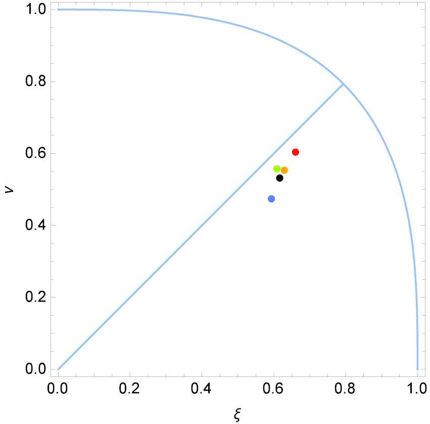
Position of the associated qROFVs
Step 6: We used the graphical ranking method to rank the qROFVs. Figure 6 shows that all qROFVs are below the equal line and thus rank based on the hesitancy index. The qROFVs with less hesitancy index ranked highest. The hesitancy degrees of qROFVs are as follows:
Remark 3.
It can be easily observed from Table 9 that optimal alternative remain same for all values of parameter
| q | π(χ1) | π(χ2) | π(χ3) | π(χ4) | π(χ5) | Developed Ranking |
|---|---|---|---|---|---|---|
| 1 | 0.10617 | 0.01938 | 0.14110 | 0.14645 | 0.10162 | |
| 2 | 0.65516 | 0.54507 | 0.70729 | 0.64501 | 0.61932 | |
| 3 | 0.85052 | 0.78930 | 0.88100 | 0.84412 | 0.83461 | |
| 4 | 0.92558 | 0.88906 | 0.94338 | 0.92204 | 0.91676 | |
| 5 | 0.95887 | 0.93592 | 0.96909 | 0.95738 | 0.95383 |
Sensitivity analysis.
7. COMPARISON ANALYSIS
This paper provides us the improved knowledge measure for qROFSs. Khan el al. [52] was first discussed the knowledge measures for qROFSs. According to them, the knowledge measure decreases with higher values of the hesitancy index, that is, the maximum information content leads to maximum knowledge. But they have not considered the information clarity facets of knowledge measure. But, as we discussed in Section 3, our proposed knowledge measure considers both perspectives of knowledge measure, that is, information content and information clarity. Hence the proposed approach is better than the previous one.
The entropy for qROFSs was discussed by Peng and Liu [37] and Verma [22]. The maximum entropy is obtained when the membership degree is equal to the nonmembership degree, that is, ξ = v. So, in these complex situations, the entropy alone can’t handle the situation. Thus it is necessary and significant work to develop an independent technique with robust properties to take measurements of the amount of knowledge in the context of qROFSs to distinguish between them. From Remark 1, we have seen that when the membership degree is equal to the nonmembership degree, the information clarity becomes zero and the knowledge is measured from an information content perspective. The higher value of knowledge measure is attached to higher value information content. Hence our proposed knowledge measure is appropriate for such situations.
8. CONCLUSION
In this paper, the knowledge measure for qROFSs is discussed with respect to information clarity and information content. Both facets of knowledge are used to quantify the knowledge from associated qROFSs. The knowledge measure is monotonically nonincreasing with respect to hesitancy index. The maximum and minimum values of knowledge measure are attached at crisp and (0,0) cases, that is, the knowledge is maximum at sure information and minimum when there is not information. For constant values of hesitancy index (say c), the equivalence classes are generated and each class has a minimum at
CONFLICT OF INTEREST
The authors declare that they have no conflict of interest.
AUTHORS' CONTRIBUTIONS
All authors contribute equally for this study.
COMPLIANCE WITH ETHICAL STANDARDS
This article does not contain any studies with human participants or animals performed by any of the authors.
ACKNOWLEDGMENTS
The Center of Excellence in Theoretical and Computational Science (TaCS-CoE), KMUTT support this project. The Petchra Pra Jom Klao Ph.D. Research Scholarship from King Mongkut’s University of Technology Thonburi support the first author (Grant No. 39/2561). Moreover, this research project is supported by Thailand Science Research and Innovation (TSRI) Basic Research Fund: Fiscal year 2021 under project number 64A306000005.
REFERENCES
Cite this article
TY  - JOUR
AU  - Muhammad Jabir Khan
AU  - Poom Kumam
AU  - Meshal Shutaywi
AU  - Wiyada Kumam
PY  - 2021
DA  - 2021/06/11
TI  - Improved Knowledge Measures for q-Rung Orthopair Fuzzy Sets
JO  - International Journal of Computational Intelligence Systems
SP  - 1700
EP  - 1713
VL  - 14
IS  - 1
SN  - 1875-6883
UR  - https://doi.org/10.2991/ijcis.d.210531.002
DO  - 10.2991/ijcis.d.210531.002
ID  - Khan2021
ER  -