
Predictive Analytics for Product Configurations in Software Product Lines
 , Ayaz H. Khan4, *, , Rehan Ullah Khan5, , Ali Mustafa Qamar6
- DOI
- 10.2991/ijcis.d.210620.003How to use a DOI?
- Keywords
- Software product line; Predictive analytics; Data science; Feature model; Inconsistency; Information system
- Abstract
A Software Product Line (SPL) is a collection of software for configuring software products in which sets of features are configured by different teams of product developers. This process often leads to inconsistencies (or dissatisfaction of constraints) in the resulting product configurations, whose resolution consumes considerable business resources. In this paper, we aim to solve this problem by learning, or mathematically modeling, all previous patterns of feature selection by SPL developers, and then use these patterns to predict inconsistent configuration patterns at runtime. We propose and implement an informative Predictive Analytics tool called predictive Software Product LIne Tool (p-SPLIT) which provides runtime decision support to SPL developers in three ways: 1) by identifying configurations of feature selections (patterns) that lead to inconsistent product configurations, 2) by identifying feature selection patterns that lead to consistent product configurations, and 3) by predicting feature inconsistencies in the product that is currently being configured (at runtime). p-SPLIT provides the first application of Predictive Analytics for the SPL feature modeling domain at the application engineering level. With different experiments in representative SPL settings, we obtained 85% predictive accuracy for p-SPLIT and a 98% Area Under the Curve (AUC) score. We also obtained subjective feedback from the practitioners who validate the usability of p-SPLIT in providing runtime decision support to SPL developers. Our results prove that p-SPLIT technology is a potential addition for the global SPL product configuration community, and we further validate this by comparing p-SPLIT's characteristics with state-of-the-art SPL development solutions.
- Copyright
- © 2021 The Authors. Published by Atlantis Press B.V.
- Open Access
- This is an open access article distributed under the CC BY-NC 4.0 license (http://creativecommons.org/licenses/by-nc/4.0/).
1. INTRODUCTION
Software Product Lines (SPLs) [1–3] are used to configure software products in which different sets of features are configured and then integrated by different teams of product developers. This is called “product configuration” wherein each team selects its feature sets from a domain-engineered Feature Model (FM) having one or more constraints [4–6]. Product configuration itself happens during the application engineering phase. When individual feature sets are integrated to form the final product, inconsistencies can occur because domain FM constraints can collectively remain unresolved due to selection of contradictory features. Much effort is then required by teams to reconfigure their feature sets, which is a complicated, resource-intensive, and a well-known problem in SPL industry [5,7–12]. A need to solve this problem during application engineering has always been highlighted by major SPL industries [13–23].
Some Artificial Intelligence (AI) [24] techniques have since been used to solve this problem, albeit during domain engineering to ensure that the FM itself remains consistent with respect to the features being added by developers. For instance, in [25], the authors have translated the FM into description logic to resolve internal inconsistencies, and in [26,27], the authors have done the same using abductive reasoning and knowledge-base (KB) rules, respectively. A review of these AI techniques (from 1990 to 2009) is given in [28]. However, we have been unable to discover any AI-based solution to resolve inconsistencies during product configuration at runtime (using a consistent FM) at the application engineering level. Rather, the focus of SPL industry in this case has been mostly on identifying inconsistencies [8]. This research gap becomes more critical as inconsistencies can also arise due to a lack of communication between developers, a change of requirements during the configuration, and the iterative transfer of inconsistencies from one development stage to another [5].
In this paper, we focus on a novel idea that the process of selection of features for any SPL product has a characteristic regularity or pattern, similarly to how different patterns of human behavior can be easily detected in online shopping and other human-centric applications. Our idea is to create an information system that can detect and memorize, rather learn, these patterns through applicable and well-known mathematical models. In this way, the selected model can be trained to have complete knowledge of how features have been selected up to now, specifically, the different steps of feature selection that have been followed by all individual SPL developers. In addition, such a system can then identify which types of patterns lead to inconsistent or consistent configurations, and provide this information to SPL developers who are currently configuring products at runtime. In fact, AI has seen a rapid pace of research since the publication of [28], and it is possible to implement our idea by using the Predictive Analytics (PA) technology [29–31], commonly known as data science or machine learning, to predict inconsistencies which can occur in the future with a given probability at runtime [10] (detailed in Section 2.2). Our contribution is the development of an information system for SPL product configuration, called p-SPLIT (predictive Software Product LIne Tool), which uses PA to extract patterns or regularities from historical product configuration data for both consistent or inconsistent configurations. It then uses these patterns to make runtime predictions about upcoming inconsistencies during future product configurations. This is the first application of PA to application engineering phase of SPL product configuration to resolve the inconsistency-related problems. In p-SPLIT, we employ the Random Forest (RF) algorithm [32] to classify and distinguish between inconsistent and consistent patterns of feature selection, because it is efficient, robust to noise and outliers, its output patterns are actually visible and comprehensible, and has shown to outsmart at least 170 other PA algorithms in a comprehensive evaluation [33] and in other papers [32,34–36].1
From aforementioned discussion, we derive the following single research question which we address thoroughly in this paper: RQ: What is the possible value which PA technology can bring to the SPL configuration process to resolve the issue of occurrence of inconsistencies at runtime during application engineering? To answer RQ, we implemented and tested p-SPLIT on real-world, historical, product configuration data obtained from a representative, anonymous multinational SPL organization (more details in Section 3). We also conducted a subjective evaluation of p-SPLIT's results with industry-based SPL designers, who validated the usefulness of our tool with respect to usability, effectiveness, efficiency, and user satisfaction. We show that p-SPLIT is able to extract patterns of inconsistent and consistent product configurations from the historical data. These patterns can be generalized to future product configurations and are capable of indicating those runtime configurations which can potentially become inconsistent (or consistent) later on. The designers' subjective responses to these patterns do indicate the latter's potential for implementation in SPL industry.
Our anonymized dataset sample and the programming code are available at sites.google.com/site/afzaluzmaa/research/i-split/p-split which provides the more critical functions of p-SPLIT to allow reproduction of our experiments. The rest of the paper is organized as follows. In Section 2, we present the relevant background and in Section 3, we provide State-of-the-Art. The proposed p-SPLIT tool is detailed in Section 4, along with the experimental methodology. In Section 5, we present the results and evaluation of p-SPLIT. Finally, we conclude and present the future work in Section 6.
2. RELEVANT BACKGROUND
In this section, we first describe the configuration of a SPL and then present different concepts of PA.
2.1. Configuring the SPL Product
During the application engineering phase, an application developer configures an SPL product by selecting a set of features from the domain-engineered FM, according to the user preferences and predefined constraints (e.g., the selection of a single feature from an alternative group of features) [37]. In this paper, we use the following notation to describe a product configuration [8]:
The curly braces denote a product configuration, for instance, if a product
We will now use an exemplary FM presented in [7] to describe the SPL product configuration. Specifically, the FM shown in Figure 1 represents the Vendor Master (VM) module of an Enterprise Resource Planning (ERP) SPL. An ERP is a large-scale information system which integrates different business units into a single information system. Each business units automates a specific department, like human resource management, product sales and purchase, production, warehousing, customer master, and VM. VM automates the business process related to the vendors that supply a business enterprise. For more details on ERP, please refer to [38]. The description of the FM in Figure 1 is as follows:
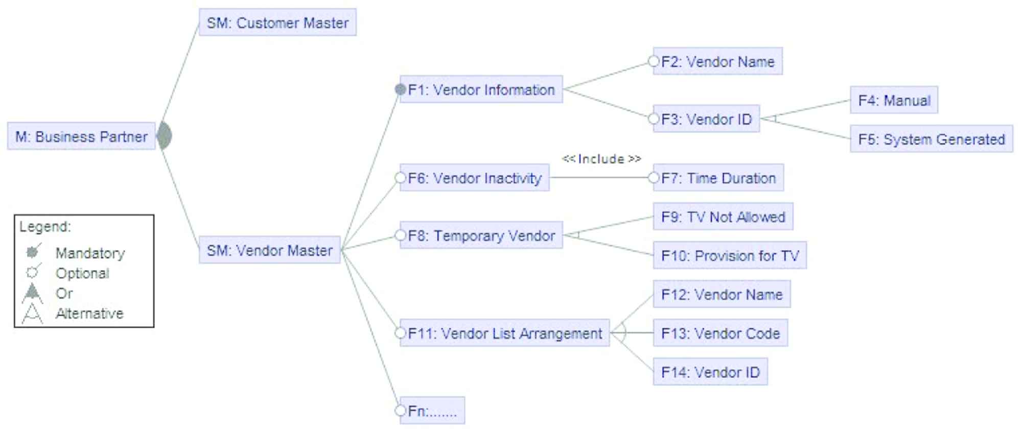
The vendor master feature model (adapted from [7]).
Using this FM of VM module as a reference, following are the examples of some consistent SPL product configurations (compliant with the constraints):
An SPL product configuration becomes inconsistent, if the selected features violate the predefined constraints (not compliant with FM). Again using FM of VM as a reference, following are some inconsistent SPL products:
2.2. Predictive Analytics
As we already defined that PA is an advanced data analytics technology used to make predictions about unknown future events. It integrates knowledge from stochastic processes, mathematical modeling, machine learning, information technology, and business management, and has a diverse application domain including customer relationship management, clinical decision support system, direct marketing, customer retention, risk analysis, fraud detection, and recommender system [29–31,39–41]. In our work, we target PA's classification process.
Classification maps input data to output predictions based on a model inferred from a given dataset. Assume an input dataset with
2.2.1. RF algorithm
There are many machine learning algorithms available to implement PA. These algorithms use different statistical approaches and hence their effectiveness varies in different scenarios [32,39,40]. As described in Section 1, we have selected the RF algorithm which constructs a multitude of Decision Trees (DTs) as predictive models [32]. DTs use concepts of entropy and information gain to select the features which are most useful in distinguishing between the labels (values) of the class variable
Algorithm 1: Pseudocode for Generating a Decision Tree for the Binary Classification
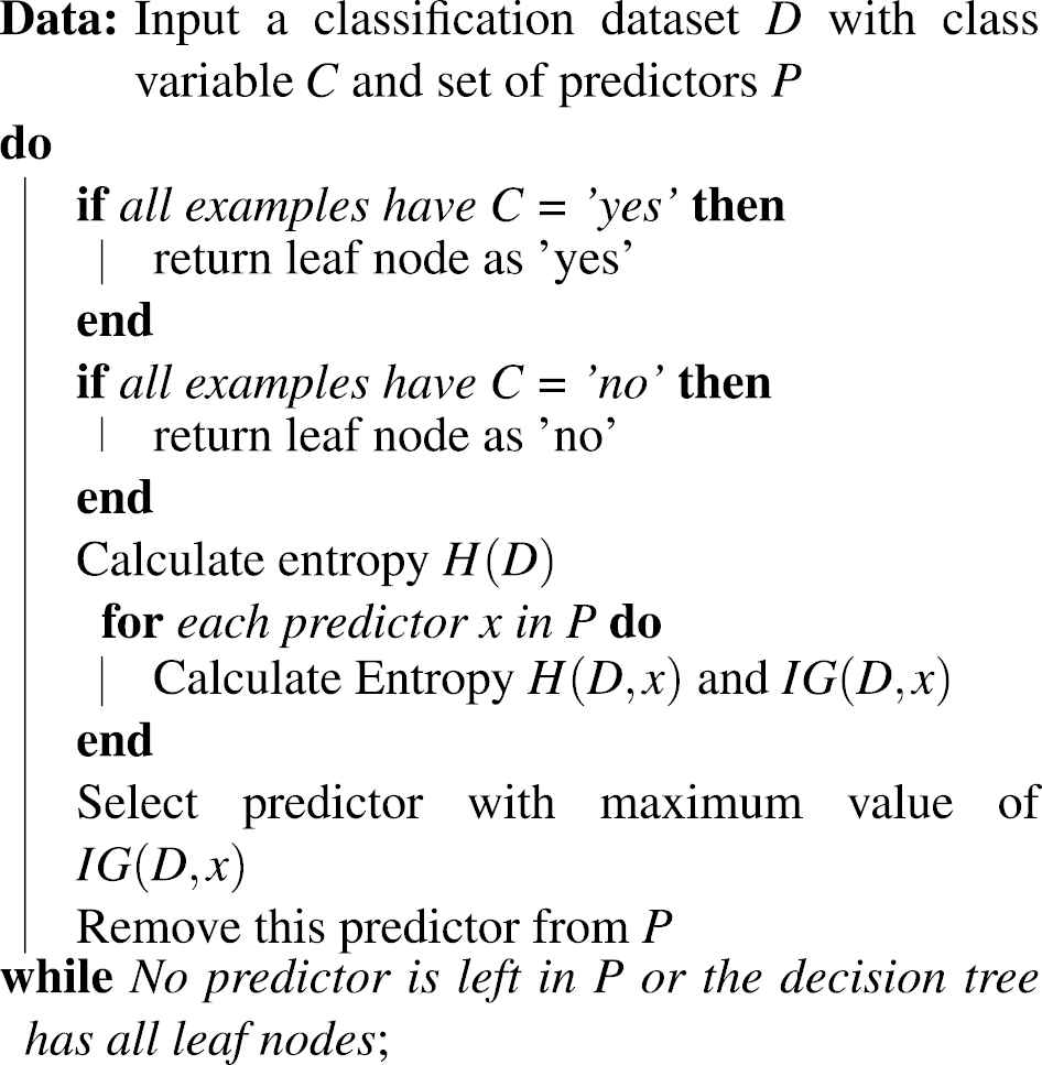
In a DT structure, the leaves represent the class labels (values of
As an example, consider the classification dataset shown in Figure 2 in which “Play Golf” is the binary class variable and the other features are weather-related predictors. The variable “Day” is an incremental counter and cannot be considered as a predictor which can have an influence on the decision to play golf. The classification problem is to use these 14 daily weather recording data to learn a DT through which we can predict whether we should play golf for a weather occurrence that will happen in the future.
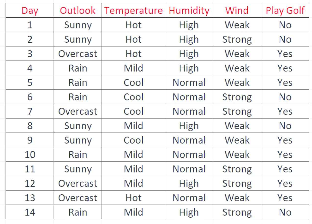
Classification dataset for playing golf.
The entropy of

Final decision tree for predicting the playing of golf.
Two well-known methods to classify a typical DT are boosting and bagging [42,43]. In boosting method, an extra weight is given to those examples which have been incorrectly predicted by the earlier predictors. In bagging methods, successive trees are constructed using a bootstrap sample which are independent of the earlier trees. RF provides an additional layer of randomness to the bagging method. A typical DT splits each node using the best split among all variables; while RF splits a node using the best among a subset of variables randomly selected for that particular node, which makes it robust against overfitting. RF is simpler in nature because it uses only a few parameters, such as the number of DTs in the RF and the number of variables in the random sample at each node. Algorithm 2 presents the pseudocode of the RF which starts from the bootstrap sampling of the dataset, followed by the selection of the best split from a random sampling of predictors. Finally, it grows DT from the split.
Algorithm 2: Random Forest—Pseudocode [34]
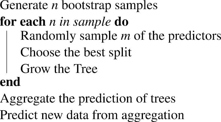
As discussed earlier, RF does not grow a single tree. Rather, it generates a collection of DTs which help in the visual and explicit representation of decisions and decision making. Similar to a typical DT, DTs in RF also construct models that can predict the value of a target variable based on several input variables. Here, each interior node corresponds to one of the input variables and the edges connect child nodes, so that all the possible values of that input variable are represented. Each leaf represents a value of the target variable on the basis of the values of input variables, represented by the path from the root to the leaf. Traversing different branches of the DT from the root node to the leaves provides different attribute combinations which classify the class labels.
2.2.2. RF evaluation
We evaluated RF on the basis of six representative performance measures, namely Accuracy, Classification Error (CE), Kappa, Area Under the Curve (AUC), Precision, and Recall. Accuracy measures the systematic errors and can be calculated as:
Precision, recall, kappa and AUC are also good classifier measures for SPL product inconsistency problem owing to its binary nature. The decision made by the binary classifier can be represented in a structure known as confusion matrix, which contains four categories, i.e., True Positive (TP), True Negative (TN), False Positive (FP), and False Negative (FN). TP and TN represent the number of correct classification of positive and negative examples, respectively. Similarly, FP and FN represent the number of incorrect classification of positive and negative examples, respectively. Precision and recall, which measure the exactness and completeness of the classifiers, respectively, are then defined as:
Because of the slightly imbalanced nature of our datasets (most of the data belong to one class), we also used Kappa statistics and AUC to measure the classification performance [40]. Kappa is calculated as:
Finally, AUC plots the TP rate vs the FP rate as the threshold value for item classification is 0 or is increased from 0 to 1. The TP rate increases quickly for the good classifier, and for the bad one, it increases linearly.
3. SPL: STATE-OF-THE-ART
Table 1 presents the state-of-the-art techniques to cater the SPL issues including inconsistent product configuration. In Noorian et al. [25], the authors present a description logic-based framework to manage the inconsistencies by identifying and resolving them. The framework is tested using a limited feature set, i.e., 35 features. An inconsistent configuration is passed to the framework which identifies and fixes the inconsistencies and generates a minimal set of consistent features. High identification and resolution times are recorded for large-scale feature set. Trinidad and Cortés [27] propose an abductive reasoning approach to identify an inconsistency with the possible reason. The proposed solution does not fix inconsistencies, moreover, an exemplary FM with a limited set of features is used for validation. Elfaki et al. [26] present a knowledge-based solution to fix the inconsistencies. The primary objective of the research is to correct an inconsistent FM due to dead and inconsistent features. For this, the given FM is converted into a KB to generate a list of inconsistent and dead features. An exemplary FM with 35 features is used to test the solution.
| Ref. | Problem Solved | Technology Used to Solve the Problem |
|---|---|---|
| [44] | Variability Mining | Recommendation System |
| [45] | Requirements Analysis | Framework Based on Cluster Analysis |
| [46] | Product Configuration | Feature Subset Recommendation based on Association Rule Mining |
| [47] | Manufacturing | Neural Network and Rules Induction |
| [48] | Product Requirements | Decision Model |
| [49] | Feature Model Design | Text Mining |
| [6] | Product Variability | Semantic Analysis |
| [25] | Product Inconsistencies | Description Logic; tested on limited feature set |
| [27] | Product Inconsistencies | Abductive Reasoning; Only identifies the inconsistencies, tested on limited feature set |
| [26] | Product Inconsistencies | Knowledge-base; focuses on inconsistent feature model |
| p-SPLIT | Product Inconsistencies | Predictive Analytics; detailed in next Section |
SPL Issuesol; column “Ref.” is the citation number; “Problem Solved” means the SPL problem solved.
From a general perspective, there are several research papers which strongly motivate the application of novel IT and CS-related technologies to solve software-related problems for the customers. For instance, the work done in [50] stressed the importance of using AI in order to model the platform development process in SPLs. In our case, platform development is synonymous with feature modeling, and AI is synonymous with PA, which can be easily considered a sub-branch of AI in the context of Machine Learning [24]. Besides this, the importance of using data mining (a traditional name for PA) to predict the customers' business requirements in advance was stressed in [51,52]. In these papers, the authors propose a customer relationship framework or model that uses data mining to anticipate in advance the business requirements of the customer. In our case, we are doing the same by using PA to predict SPL features, which are synonymous with requirements.
Also, the work done in [53] has critically evaluated the impact of web-based PA (data mining) tools for the software industries and the clients. It mentions that such a venture can face complex issues, e.g., risk of investment, reduced budget, difficulty of communicating between different stake holders, and reduced knowledge of data mining outputs and processes.
From a technical perspective, the research articles applying PA or related technologies to SPL-related issues are quite limited (Table 1). Perhaps the work most related to our approach is the one by Kastner et al. [44], in which the authors introduce a new approach called variability mining. Here, given the domain knowledge of SPL features and the corresponding programming code, an internal representation of feature mappings and code structures is first built. Based on this model, a recommendation system is then used to recommend (or mine) the fragments of code, which the SLP developer should consider for configuring the product. Developers have the independence to accept or reject the recommendations, along with incorporating domain knowledge manually in the process. The system obtains a high average recall of 90% but a low average precision of 42%.
In another related paper [45], the authors present a framework based on cluster analysis [30] to analyze functional requirements in the SPL development process. This outputs different clusters of feature selections, particularly based on the perspectives of the stakeholders.
Another important work is presented in [46], where the authors use association rule mining to recommend the potential subset of features to configure an SPL product at runtime. The authors validate their work in an industrial setting but do not implement any comprehensive decision support system that uses the results in a more usable and personalized manner. The authors have not presented the results in enough detail to clearly understand the impact of the proposed technology in an industrial setting. Also, the work done in [47] validates the use of data mining techniques to solve complex problems in semiconductor wafer manufacturing SPLs. Some major issues include nonlinear interactions between different design groups, fast-changing business processes, a large variety of products, and the increasing volume of data (big data). The authors demonstrate how self-organizing neural networks and rule induction [24,30] can be used to solve these problems and increase the yield from 3% to 15% along with solving problems 10 times more efficiently.
In a somewhat more historical work [48], the author proposes the design and implementation of a specification infrastructure for SPLs, which can be reused by SPL developers later on to configure products in a better way. The specification can be structured to suit the needs of the customers, including a systematic method of reuse. The authors present a limited case study to validate the technology. However, it cannot handle the complex variability of SPL design, which is definitely not a hindrance for our PA-based approach, given that PA can also be based on techniques from Big Data Analytics and provides more robust models as compared to a simple specification.
In Maazoun et al. [49], the authors explore text mining technique to design the FM. They analyse and compare the quality of the FMs designed using text mining with the FMs developed by experts. In Zhou et al. [6] authors discuss the importance of FM in identifying variability and commonality of SPL product. They use sentiment analysis to incorporate client's preferences.
4. PREDICTIVE SOFTWARE PRODUCT LINE TOOL (p-SPLIT)
In this section, we describe the proposed predictive framework. Figure 4 shows the architectural view of different modules of p-SPLIT.
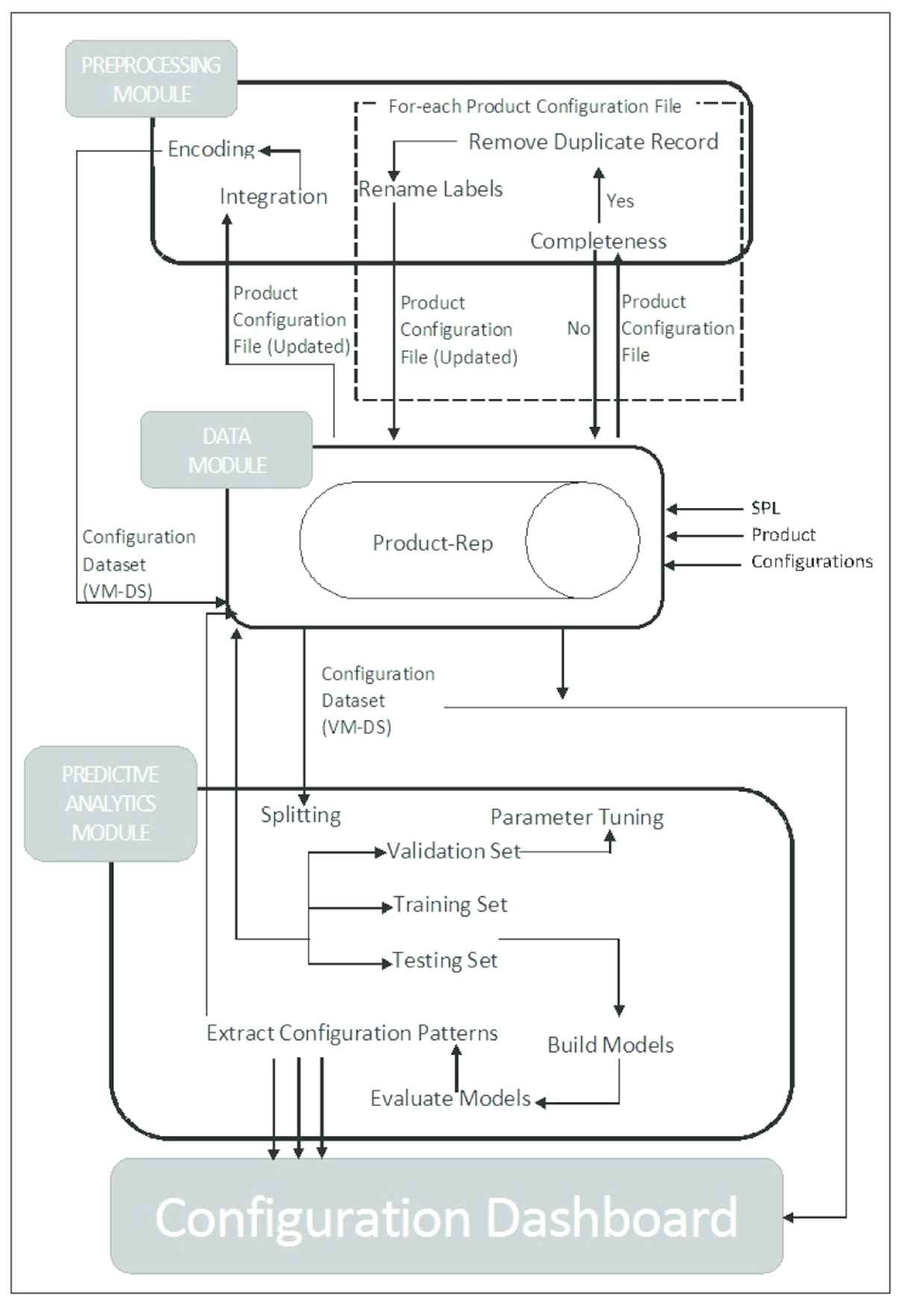
Architecture of Predictive Software Product Line Tool (p-SPLIT): predictive software product line tool.
4.1. Data Module
Data Module (DM) stores SPL configurations to the Product-Rep(ository). We acquired real-world data of an anonymous, multinational ERP-based SPL.2 The essence of p-SPLIT is to give the developers decision support during the product configuration process. Moreover, configuration is a collaborative process, which involves multiple developer teams. Each team is solely responsible for the assigned configuration module. Keeping all these things in mind, it does not make sense to design a single dataset for a complete SPL product, because irrelevant configuration rules (or those related to other modules) being displayed on the developer's dashboard introduce more confusions and increase the complexity of the overall process. Therefore, we advocate the mining of SPL product configuration on a module by module basis. For p-SPLIT experiments, we acquired the configuration data of VM module from the configuration repository of our anonymous company. This data contained both types of configurations, i.e., consistent and inconsistent, stored in a text file. It contained a total of 178 different configurations.
4.2. Preprocessing Module
Before generating a complete dataset, we preprocessed and cleaned the individual configuration text files. For this, Preprocessing Module (PM) implemented programs in Java and C#.
PM checked the completeness of the data by analyzing the metadata and data stored in the files. The metadata contains the information about the SPL product configuration, including the number of features configured and the number of inconsistencies present in the configuration. PM imported the data from a text file to regenerate the configuration information and matched this information to the original metadata information to confirm the completeness and occurrence of missing features. In case, a data file was found to be faulty, PM used backup files. PM also checked the data for data inconsistencies by removing the duplicate entries of features.
PM also renamed the feature labels and combined the name of a feature with its constraint. For instance, for feature
After this, PM integrated these text files to produce a single data file. These configurations are imported into an Excel file, wherein each configuration was mapped to a row with a unique configuration ID. PM then transformed and encoded the data into binary data. A binary variable is created for each of the configuration features. After that, data reduction is applied and configuration ID column is removed from the dataset. For the given configuration with
Furthermore, a column is introduced to represent the class label, which stores “Consistent” for the consistent configurations and “Inconsistent” for the inconsistent SPL product configurations. This dataset is stored in Product-Rep as VM-DS (VM DataSet) which is further divided into training, validation, and testing sets.
4.3. Predictive Analytics Module
Predictive Analytics Module (PAM) is the core module of p-SPLIT which implements RF DT to generate the decision support rules for SPL developers' team. It acquires the dataset of inconsistent and consistent product configurations from the DM (Product-Rep repository) to build a DT model. This model is validated on a testing set. The performance of models is compared in terms of their accuracy, precision, and recall. After the model validation, the decision rules are extracted from the model. Finally, these decision rules are passed to the Configuration Dashboard (CD). In PAM, we employed the RapidMiner tool [54] to estimate the predictions, and then visualized the results in C# language to provide decision support to the developers' teams.
4.3.1. Process design
The process flow of PAM starts with the reading of relevant dataset from the file. Then, the dataset is split into training, validation, and testing sets (a representative approach [55,56]). The primary parameters are tuned using the validation dataset. Using the training set with the tuned values of parameters, we then generate the RF models. These models are then applied on testing sets, and the performance for both sets is evaluated (recall that our performance measures are Accuracy, Kappa, AUC, Precision, and Recall). Finally, we generated the configuration rules from the trees which had better performance. We then hardcoded these into the CD. We performed all of these PAM experiments on a Windows 8 machine with Intel Core i7 CPU, 2.4 GHz processor, and 16GB of RAM.
4.3.2. Parameters tuning
The primary parameters of RF, such as the number of trees, criteria on which the attributes will be selected for tree splitting, the maximal depth of the tree, and prepruning were tuned according to the dataset and the nature of the problem. To determine the range of trees within a RF, we used the suggestions of [36]. We also tuned the maximal depth parameter with different bounds. To tune the feature selection criterion for splitting, we experimented PAM with information gain and gini index. We deselected the pruning, prepruning, and local seed selection options to obtain fully-grown DTs in RF. We allowed RF to guess the subset ratio to generate the trees.
To determine the range of trees within a RF, we used the suggestions of [36] and set the value to 70 which is a good balance between AUC, processing time, and memory usage. For the maximal depth parameter, we put no bound on the depth of the tree, i.e., a tree of maximum depth is generated. We used information gain as the feature selection criterion for splitting over gini index, as gini index targets continuous features while entropy targets features which occur in classes [57]. It should also be mentioned that in [58], the authors analyze the frequency of agreement/disagreement of the gini index and the information gain function. They found that the disagreement is only 2% and concluded that it is not possible to decide which one should be preferred. Therefore, our selection of information gain can also be attributed to our own preference and the previous experience. The optimal values of RF parameters which we selected are shown in Table 2.
| Number of Trees | 70 |
| Criterion | Information Gain |
| Maximal Depth | No Bound |
PAM: optimal values for parameters.
4.4. Configuration Dashboard
CD in Figure 4 is an interface to provide the textual and graphical representation of the product under configuration. It also provides support to the developers on the basis of the decision rules, which are fetched from PAM. CD has the following features:
It provides the current status of the configuration including: the number of features configured, number of inconsistencies in the current configuration along with the detail of each inconsistency type, and the Inconsistent features with their constraints.
Configuration patterns, which lead to an inconsistent configuration.
Configuration patterns, which lead to a consistent configuration.
We have implemented CD in C# programming language and it fetches all the relevant information from the DM (configuration repositories) and PAM.
5. RESULTS AND DISCUSSIONS
We ran PAM experiments based on the experimental methodology explained in the previous section. In this section, we discuss the results of these experiments.
5.1. VM-DS Results and Discussion
In this subsection, we answer the research question RQ1. For this, we experimented VM-DS with the tuned value of the parameters (shown in Table 2). The dataset is splitted into two parts, i.e., training and testing. After that, we trained RF classifier on the training set and tested on the testing set. Finally, we analyze the performance of the model in terms of Accuracy, CE, Kappa, AUC, Precision, and Recall. Table 3 shows the result.
| VM-DS | |
|---|---|
| Accuracy | 85% |
| CE | 14% |
| Kappa | 0.66 |
| AUC | 0.978 |
| Precision | 81% |
| Recall | 73% |
PAM-results.
The accuracy of VM-DS model is 85% and CE is 14% with 0.66 kappa value and 0.978 AUC. The precision and recall of the VM-DS model are 81% and 73%, respectively.
Now, we discuss the possible role of PA through RF to solve the product configuration problem. PAM results show that the model generated from VM-DS has a good performance. Therefore, we used it to extract the configuration rules, which are further encoded to the CD. Figure 5 shows a snapshot of the RF generated with VM-DS. In this figure, the leaf labels represent either an inconsistent pattern (blue color) or a consistent pattern (red color). A complete red or blue leaf node represents a complete pattern for consistent or inconsistent configuration, respectively (i.e., no more features are needed to classify this particular consistency or inconsistency). Leaf nodes containing both red and blue color imply that more features are needed to acquire complete patterns. However, if one color has a larger frequency (and hence a larger size of the bar) than the other in this hybrid combination, then the former can be considered as the predicted class; RapidMiner has labeled these hybrid nodes accordingly.
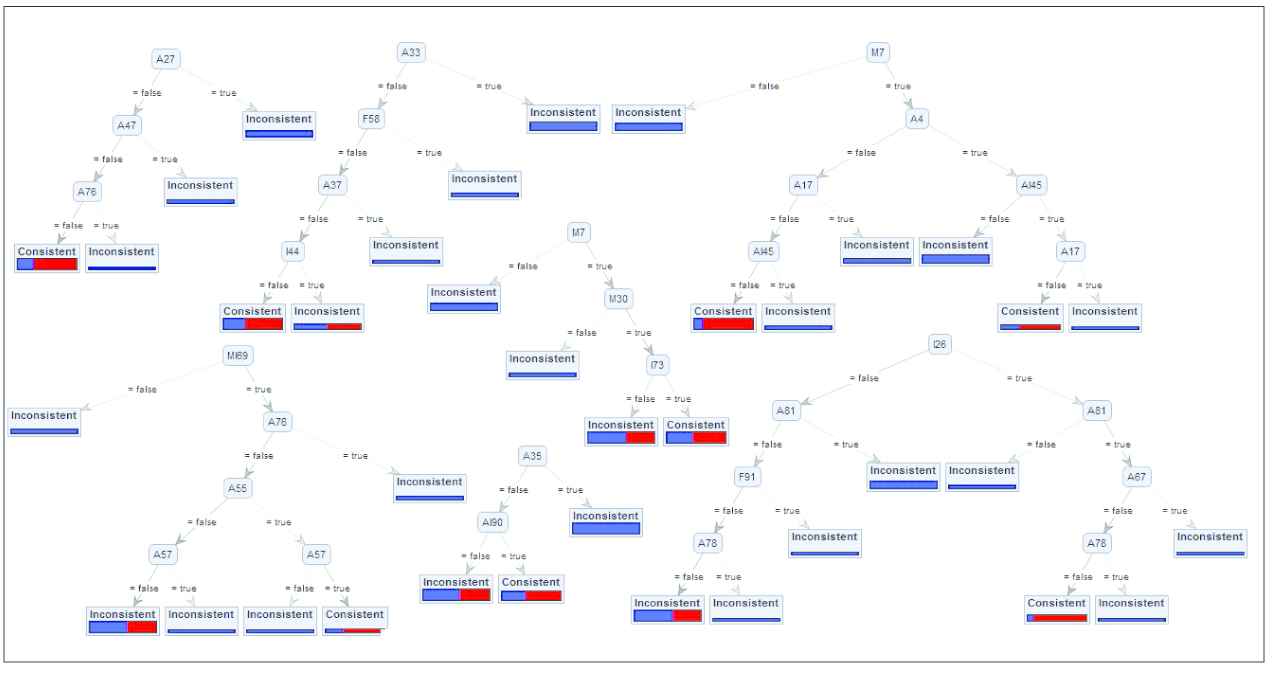
A snapshot of the tree output by random forest algorithm.
To explain the extraction of the configuration rules and their usability, we randomly picked a DT from the RF.
Figure 6 shows a sub-tree of the RF tree shown in Figure 5, which presents three classification patterns for inconsistent configuration and two for the consistent one. The dynamics of the model are as follows:
The selection of A37 leads to inconsistencies 75% of the time.
Deselection of A37 along with M10 leads to inconsistencies 63% of the time.
If M10 and I74 are selected, then not selecting A37 leads to consistent configuration 62% of the time.
If M10 is selected, then not selecting A37, I74, and M7 leads to inconsistencies 57% of the time.
The partial classification indicates that most of the configurations in our VM-DS-Comp data have a strong probability of turning out to be inconsistent.
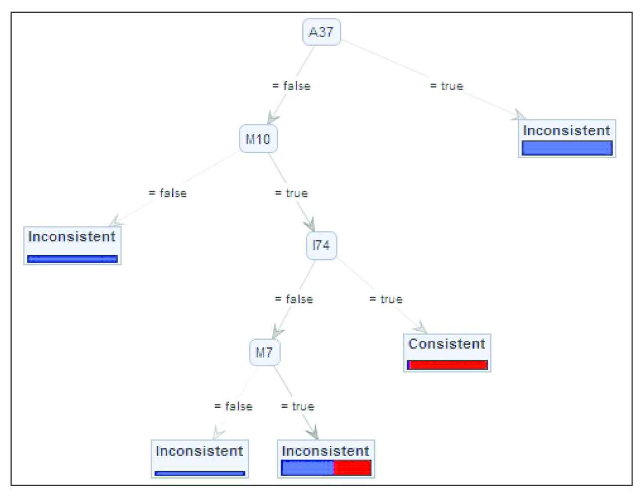
A sub-tree of the random forest tree shown in Figure 5.
These configurations rules along with their statistics and visuals are encoded to the CD, which helps developers during a product configuration and provides a runtime decision support.
We discuss the functionalities of CD with the help of a working example of an SPL product configuration. Figure 7 shows the configuration process of VM-ERP module of CL-T-ERP. The top left of Figure 7(A) shows the tracking information of VM-ERP, i.e., CL-T-ERP (product name) and T-ERP (SPL name), the top right shows the information of the features already configured within VM-ERP. The bottom of Figure 7(A) shows a list of the potential features which are not part of VM-ERP, but can still be selected. Figure 7 also shows an integrated support of PA-based CD. The bottom of Figure 7(B) shows how a runtime help is available to support the configuration decisions.
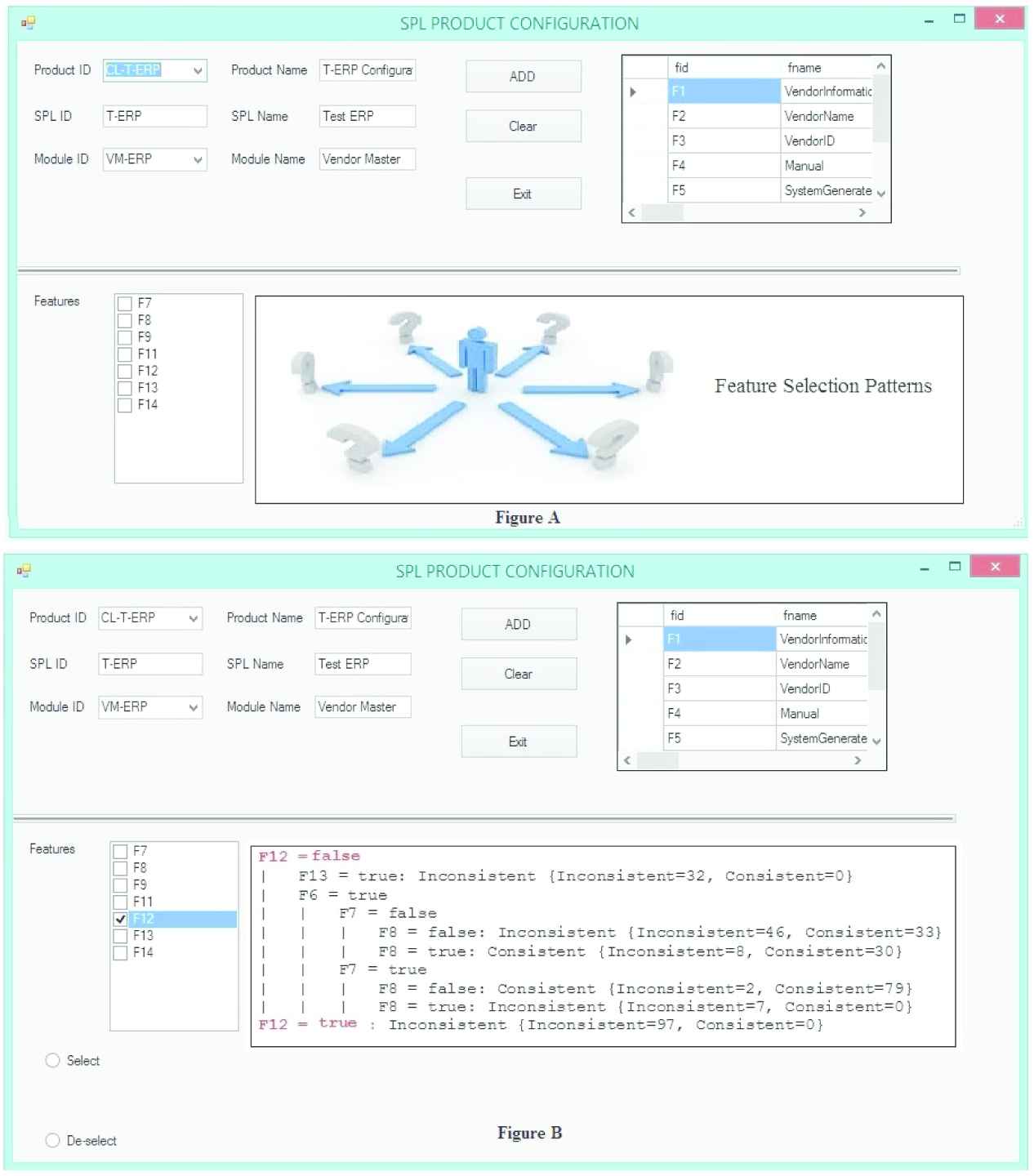
Software product line configuration dashboard (SPL CD) of predictive software product line tool (p-SPLIT).
As the developer team selects
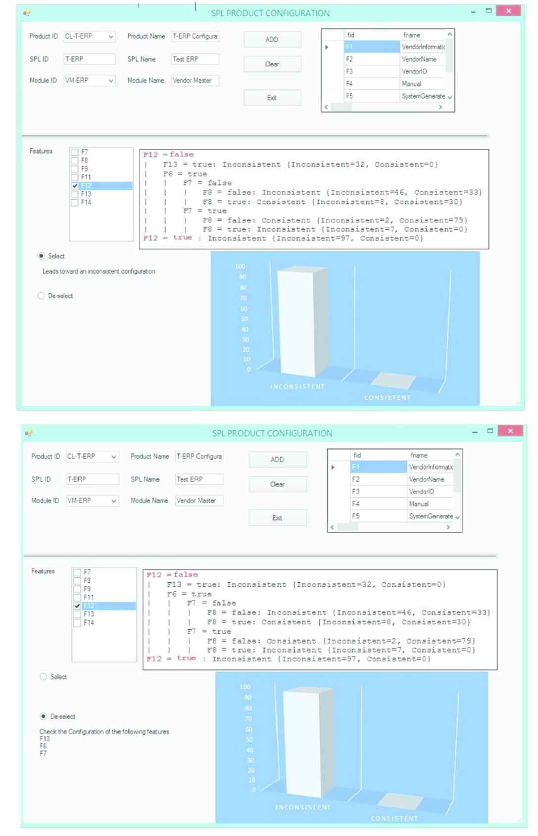
Detailed configuration dashboard (CD) of predictive software product line tool (p-SPLIT).
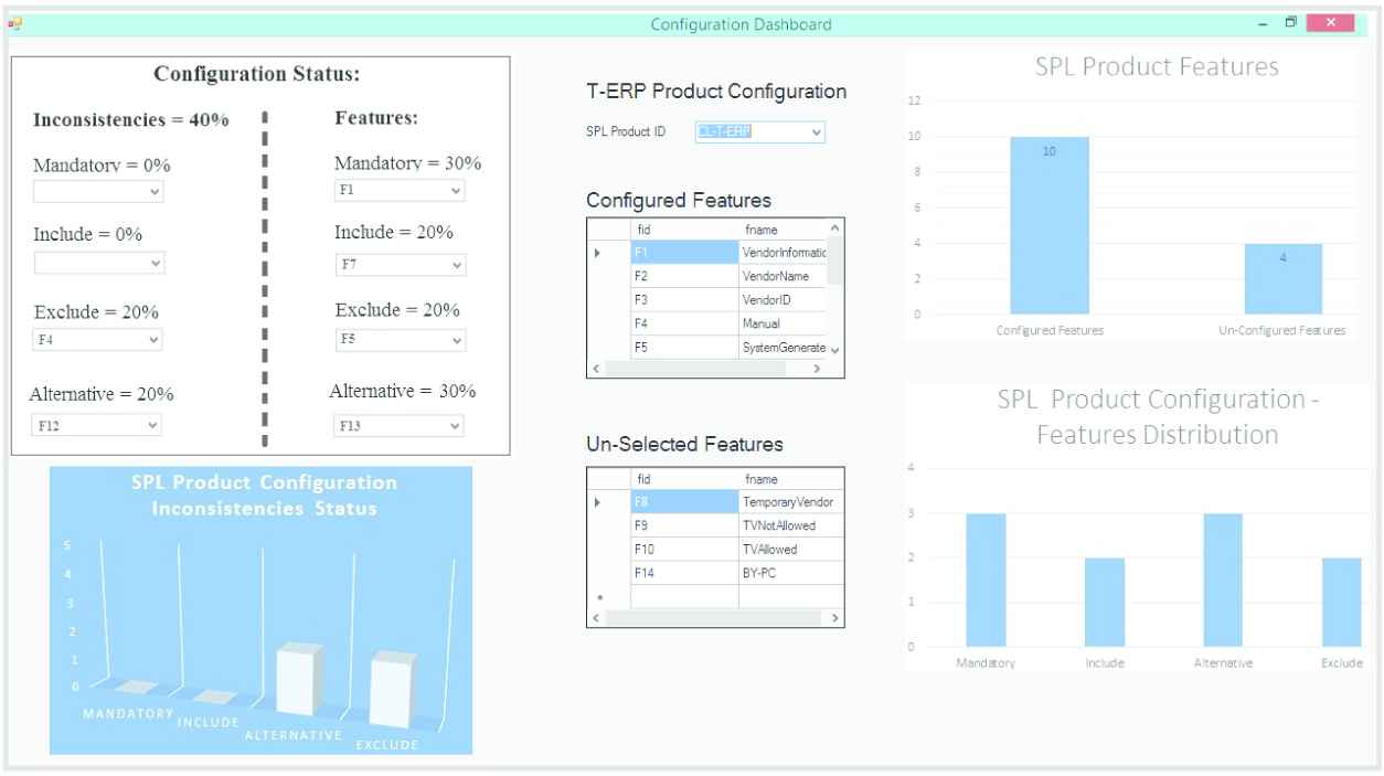
Product details shown in configuration dashboard.
CD also lists down the features which introduce the listed inconsistencies in the Inconsistencies combo boxes. The bottom left of the figure shows a visual representation of the inconsistencies. The top left of the figure (labeled as Features) shows the division of the configured features on the basis of their constraint types. CL-T-ERP configuration contains 30% mandatory features, 20% include and exclude features, and 30% alternative features. The bottom right of the figure presents graphs of the CL-T-ERP configured features distribution. The combo boxes of CD populate only the first 100 records to keep it efficient, while developers can customize combo boxes to show all of the records.
Based on this example and subsequent discussion, we can now answer our research question by stating that a PA-equipped CD can facilitate SPL developers teams in three ways: 1) By displaying patterns of feature selection leading to inconsistent product configurations, 2) By displaying patterns of feature selection leading to consistent product configurations, and 3) Predicting inconsistencies in products that are currently under configuration.
5.2. Subjective Evaluation and Benefits of p-SPLIT
To acquire subjective feedback for p-SPLIT, we implemented p-SPLIT in our client company whose FM and datasets were used to run our experiments. Initially, we developed a testing environment to configure a medium-scale ERP product for a team of ten developers (comprising four junior and six senior developers). We setup ten test servers and a single database server, where one test server was assigned to every developer. We connected all test servers to the database server for sharing SPL repositories and equipped each with p-SPLIT interface. We populated the database server with configuration repositories of p-SPLIT. We also populated the p-SPLIT repositories with the test FM data for medium-scale configuration. We started the testing process with domain engineering of a medium-scaled FM. After that, we configured a product for an exemplary client. runtime decision support was available throughout the configuration process. After the successful execution of p-SPLIT in the testing environment, we acquired subjective feedback from the developers involved in the test configuration.
We acquired this feedback through a subjective questionnaire based on standard guidelines [59]. The developers provided feedback for p-SPLIT results on a scale of 1 (strongly disagree) to 5 (strongly agree) for the following four questions:
Q1: The statistics displayed on CD are helpful.
Q2: The PAM results, displayed on CD, provide an appropriate runtime feature selection and deselection support.
Q3: The decision support provided by CD is efficient as compared to the manual configurations.
Q4: The decision support provided by CD has a practical applicability to the business domain.
We acquired feedback from all the ten developers and calculated the average response for each question. Q3 received an average of 5, i.e., all developers strongly agreed that the decision support by p-SPLIT makes the configuration process more efficient as compared to traditional method. Q1 and Q2 received an average of 3.8, while Q4 received an average of 4. Although we agree that these results are acquired for only a single evaluation in a limited setting, they do indicate that p-SPLIT has the potential to provide the relevant decision support for SPL developers.
Besides this subjective evaluation, we present a comparison of two widely used industrial tools with p-SPLIT to highlight the advantages of proposed solution. Pure::variants [60] and Gears [61] have widespread applications as compared to other tools [62,63]. Table 4 shows that p-SPLIT can facilitate SPL developers teams in three ways:
Classifying patterns of feature selection leading to inconsistent FM.
Classifying patterns of feature selection leading to consistent FM
Predicting inconsistencies in FM that are currently under configuration.
| pure::variants | Gears | p-SPLIT | |
|---|---|---|---|
| Generate Pattern of Inconsistent Features | X | X | ✓ |
| Generate Pattern of Consistent Features | X | X | ✓ |
| Predicting Inconsistencies | X | X | ✓ |
| Identify Inconsistencies | ✓ | ✓ | ✓ |
| Resolve Inconsistencies | ✓ | ✓ | X |
A Comparison of state-of-the-art gears and pure::variants industrial tools with p-SPLIT.
p-SPLIT also provides current status of the configuration including:
Number of features configured.
Number of inconsistencies in the current configuration with the detail of each inconsistency type.
Inconsistent features with their constraints.
6. CONCLUSIONS AND FUTURE WORK
In this paper, we present a novel technology for the SPL business domain called p-SPLIT, which uses PA to address the SPL product configuration issues by providing decision support to SPL developers' team at runtime. p-SPLIT provides this runtime by offering a CD, which helps the developers using the configuration rules generated by PA. p-SPLIT classifies the pattern of configurations of feature selection leading to inconsistent and consistent product configurations. It also predicts the inconsistencies of FM which are currently under configuration by showing them on CD.
As a future work, we intend to expand our experiments with large-scale datasets (big data) and equip the CD with relevant inter-module configurations patterns. Work on the the inter-operability of p-SPLIT with other industrial tools such as Gears and Purevariants is another future direction. We are also planning to share p-SPLIT through a web interface which can be integrated with SPLOT and BeTTy and made freely available for academic and research purpose.
CONFLICTS OF INTEREST
The authors declares that they have no conflict of interest.
Footnotes
This has been proven in several of our industrial projects conducted in the following companies: https://nexdegree.com/, https://codexnow.com/, and https://frontiertechnologyinstitute.com/
Due to a Nondisclosure Agreement, we cannot disclose the name of the company
REFERENCES
Cite this article
TY  - JOUR
AU  - Uzma Afzal
AU  - Tariq Mahmood
AU  - Raihan ur Rasool
AU  - Ayaz H. Khan
AU  - Rehan Ullah Khan
AU  - Ali Mustafa Qamar
PY  - 2021
DA  - 2021/06/28
TI  - Predictive Analytics for Product Configurations in Software Product Lines
JO  - International Journal of Computational Intelligence Systems
SP  - 1880
EP  - 1894
VL  - 14
IS  - 1
SN  - 1875-6883
UR  - https://doi.org/10.2991/ijcis.d.210620.003
DO  - 10.2991/ijcis.d.210620.003
ID  - Afzal2021
ER  -