
Order-αCQ Divergence Measures and Aggregation Operators Based on Complex q-Rung Orthopair Normal Fuzzy Sets and Their Application to Multi-Attribute Decision-Making
 , Abdu Gumaei2, *,
 - DOI
- 10.2991/ijcis.d.210622.004How to use a DOI?
- Keywords
- Complex q-Rung orthopair normal fuzzy sets; Order-αCQ divergence measures; Aggregation operators; Multi-attribute decision-making
- Abstract
Complex q-rung orthopair fuzzy set (CQROFS) contains the grade of supporting and the grade of supporting against in the form of polar coordinates belonging to unit disc in a complex plane and is a proficient technique to address awkward information, although the normal fuzzy number (NFN) examines normal distribution information in anthropogenic action and a realistic environment. Based on the advantages of both notions, in this manuscript, we explored the novel concept of a complex q-rung orthopair normal fuzzy set (CQRONFS) as an imperative technique to evaluate unreliable and complicated information. Some operational laws based on CQRONFSs are also explored. Additionally, some distance measures, called complex q-rung orthopair normal fuzzy generalized distance measure (CQRONFGDM), complex q-rung orthopair normal fuzzy symmetric distance measure (CQROFNFSDM), two types of complex q-rung orthopair normal fuzzy order- divergence measures (CQRONFODMs), and their special cases are discussed. Moreover, weighted averaging, weighted geometric, generalized weighted averaging, and generalized weighted geometric operators based on CQRONFSs are also presented. In last, we solved a numerical example of a multi-attribute decision-making (MADM) problem is shown to justify the proficiency of the presented operators. The advantages, comparative and sensitive analyses are used to express the efficiency and flexibility of the explored approach.
- Copyright
- © 2021 The Authors. Published by Atlantis Press B.V.
- Open Access
- This is an open access article distributed under the CC BY-NC 4.0 license (http://creativecommons.org/licenses/by-nc/4.0/).
1. INTRODUCTION
In our everyday life, most people are regularly confronted with MADM issues, which may include various other options and numerous assessment components. Because of the multifaceted nature of human social exercises and the vulnerability of indigenous habitats, the way to manage such dubious data has gotten the key to taking care of the MADM issues. Zadeh [1] explored a supporting-based fuzzy set (FS), which viably portrayed the fuzzy data and dubious condition, and hence the advantage to suggest a superior choice. Additionally, Atanassove [2] modified the theory of FS to intuitionistic FS (IFS) containing three components, that is, participation degree, nonenrollment degree, and hesitation degree. IFS has been broadly considered, and various scholars have extended into different kinds of notions [3–6]. Additionally, Yager [7] situated the modified version of IFS is called Pythagorean FS (PFS) and meet the conditions that the square sum of its supporting grade and supporting against grade is not exceeded from unit interval. Several scholars have utilized it in different fields [8–12]. Further, Yager [13] situated the modified version of PFS is called q-rung orthopair FS (QROFS) and meet the conditions that the q-power sum of its supporting grade and supporting against grade is not exceeded from unit interval. Several scholars have utilized it in different fields [14–18].
From the above winning investigations, it has been breaking down that the above examination has been led under the uncertainties or their expansions which can just arrangement with the vulnerability that exists in the data. None of these models can speak to the incomplete numbness of the information and its variances at a given period. Nonetheless, in complex informational indexes, for example, information from the clinical research, database for biometric and facial acknowledgment, and so on. Vulnerability and dubiousness in the information happen simultaneously with changes to the stage (periodicity) of the information. To deal with the periodicity of the information into the decision-making problems, Ramot et al. [19] presented the idea of the complex fuzzy set (CFS), a modified version of the FS, displayed by complex-valued supporting grade with a co-domain unit circle in an unpredictable plane. Additionally, Alkouri and Salleh [20] modified the theory of CFS to complex IFS (CIFS) containing three components, that is, complex-valued participation degree, complex-valued nonenrollment degree, and complex-valued hesitation degree. CIFS has been broadly considered and various scholars have extended it into different kinds of notions [21–23]. Additionally, Ullah et al. [24] situated the modified version of CIFS is called complex PFS (CPFS) and meet the conditions that the square sum of its real part (also for the imaginary part) of the supporting grade and real part (also for the imaginary part) of the supporting against grade is not exceeded form unit interval. Several scholars have utilized it in different fields [25]. Further, Liu et al. [26,27] situated the modified version of CPFS is called complex QROFS (CQROFS) and meet the conditions that the q-power sum of its real part (also for the imaginary part) of the supporting grade and real part (also for the imaginary part) of the supporting against grade is not exceeded form unit interval. Several scholars have utilized it in different fields [28].
The point of this exploration is to introduce a novel decision-making technique to take care of the MADM issues utilizing CQRONFSs which is a mixture of CQROFSs and normal fuzzy numbers (NFNs) [29] with powerful averaging and geometric operators. The CQRONFSs is a speculation of the QRONFS thinking about the supporting grade and supporting against are complex-valued and are expressed in polar coordinates with NFNs. The amplitude term gives the degree of belongingness of an item in a CQRONFS and the stage terms are commonly identified with periodicity. These stage terms recognize the CQRONFS and customary QRONFS theories. Uncertainties hypothesis manages just each measurement in turn which brings about data misfortune in certain examples. Be that as it may, all things considered, we run over complex characteristic marvels where it gets basic to add the second measurement to the declaration of participation and non-enrollment grades. By presenting this subsequent measurement, the total data can be expert projected in one set, and henceforth, loss of data can stay away from. To delineate the essentialness of the stage term, we give a model. “Consider XYZ organization chooses to set up biometric-based participation gadgets (BBPGs) in the entirety of its workplaces spread everywhere throughout the nation. For this, the organization counsels a specialist who gives the data regarding (i) demonstrates of BBPGs and (ii) creation dates of BBPGs. The organization needs to choose the most ideal model of BBPGs with its creation date all the while. Here, the issue is two-dimensional, which cannot be demonstrated at the same time utilizing customary QRONFS theories. The most ideal approach to speak to the entirety of the data gave by the master is by utilizing CQRONFS theories. The amplitude terms in CQRONFS might be utilized to give the organization's choice concerning the model of BBPGs, and the stage terms might be utilized to speak to the organization's judgment concerning creation date of BBPGs.”
When a decision-maker gives
If we choose the value of the imaginary part will be zero in CQRONFS, then the CQRONFS is converted for q-rung orthopair normal FS.
If we choose the value of the imaginary part will be zero in CQRONFS for q = 2, then the CQRONFS is converted for the Pythagorean normal FS.
If we choose the value of the imaginary part will be zero in CQRONFS for q = 1, then the CQRONFS is converted for an intuitionistic normal FS.
If we choose the value of the q = 2 in CQRONFS, then the CQRONFS is converted for a complex Pythagorean normal FS.
If we choose the value of the q = 1 in CQRONFS, then the CQRONFS is converted for a complex intuitionistic normal FS.
If we choose the value of normal FS will be zero in CQRONFS, then the CQRONFS is converted for CQROFS.
If we choose the value of the normal FS will be zero in CQRONFS for q = 2, then the CQRONFS is converted for a complex PFS.
If we choose the value of the normal FS will be zero in CQRONFS for q = 1, then the CQRONFS is converted for a complex IFS. The geometrical expression of the unit disc is discussed in the form of Figure 1.
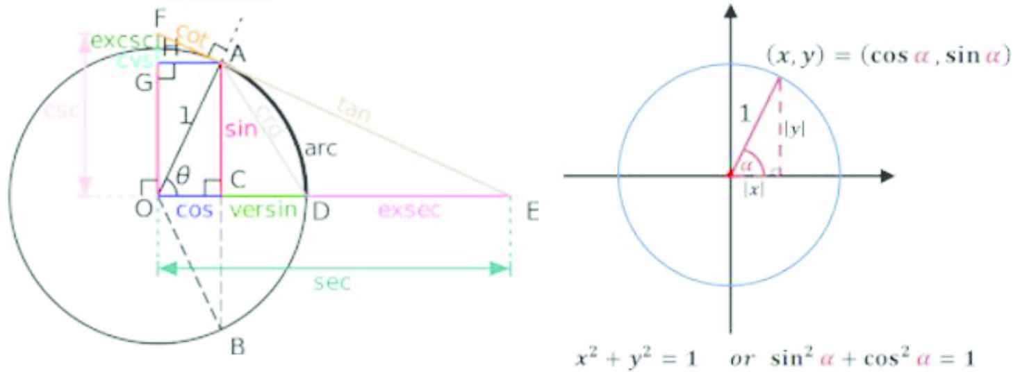
Expressions of the unit disc in complex plane in unit disc.
In this way, inspired by the attributes of the CQRONFS model and the significance of data aggregation, this paper centers around investigating the basic qualities of CQRONFSs and their aggregation operators (AOs) for dealing with the multidimensional complex informational collections. The primary accomplishments of this examination are:
To handle the uncertainties in a more precise environment using CQRONFSs and their fundamental properties are explored.
To explore some new Order-
To explore some new AOs to combine the preferences.
To explore an efficient algorithm based on explored measures and operators to solve MADM problems.
To illustrate the approach with a numerical example for evaluating the proficiency and reliability of the presented approaches.
To achieve these objectives, we provide more flexibility to the decision-maker to provide their preferences in terms of CQRONFSs to achieve the first objective. The second objective is done by proposing some new Order-
The remaining text is outlined as follows: in Section 2, we review some notions like NFN, CQROFS, and their operational laws. In Section 3, we explored the novel concept of CQRONFS is an important technique to evaluate unreliable and complicated information. Some operational laws based on CQRONFSs are also explored. In Section 4, some distance measures are called CQRONFGDM, CQROFNFSDM, two types of CQRONFODMs, and their special cases are discussed. In Section 5, some weighted averaging, weighted geometric, generalized weighted averaging, and generalized weighted geometric operators based on CQRONFSs are also presented. In Section 6, we solve a numerical example on multi-attribute decision-making (MADM) problem is shown to justify the proficiency of the presented operators. The advantages, comparative and sensitive analysis are used to express the efficiency and flexibility of the explored approach. The conclusion of this article is discussed in Section 7.
2. PRELIMINARIES
The purpose of this communication is to review some notions like NFN, CQROFS, and their operational laws. Throughout, this manuscript, the symbol
Definition 1.
[29] A NFN
Definition 2.
[29] For any two NFNs
The distance measure based on NFNs is stated by
Definition 3.
[26,27] The CQROFS
Definition 4.
[26,27] For any two CQROFNs
Definition 5.
[26,27] For any CQROFN
For finding the relationships between any two CQROFNs, we use the following inequalities:
If
If
If
If
3. COMPLEX Q-RUNG ORTHOPAIR NF N
The purpose of this communication is to present the notion of CQRONFN, which is the mixture of CQROFS and NFN to cope with uncertain and awkward information in realistic decision theory. Some basic operational laws for CQRONFN are also explored.
Definition 6.
The CQRONFN
Definition 7.
For any two CQRONFNs
Definition 8.
For any CQRONFN
For finding the relationships between any two CQRONFNs, we use the following inequalities:
If
If
If
If
Theorem 1.
For any two CQRONFNs
Proof.
Straightforward.
4. DISTANCE MEASURES BASED ON CQRONFNs
The purpose of this section is to explore some distance measures are called CQRONFGDM, CQROFNFSDM, complex q-rung orthopair normal fuzzy Order-
Definition 9.
For any two CQRONFNs
Eq. (26), must hold the following conditions:
In the CQRONFS hypothesis, enrollment and nonmembership degrees are intricate esteemed and are spoken to in polar directions. The abundance term comparing to the participation (nonmembership) degree gives the degree of things (not‐belongings) of an item in a CQRONFS, and the stage term related to enrollment (nonmembership) degree gives the extra data, by and large, related with periodicity. The stage terms are novel boundaries of the participation and nonmembership degrees, and these are the boundaries that recognize the customary QRONFS and CQRONFS hypothesis. QRONFS hypothesis manages just each measurement in turn, which brings about data misfortune on certain occasions. In any case, in day‐to‐day life, we run over complex normal marvels where it gets fundamental to add the second measurement to the statement of participation and nonmembership grades. By presenting this subsequent measurement, the total data can be extended in one set, and henceforth, loss of data can be maintained a strategic distance from. To show the hugeness of the stage term, consider an illustration of a specific organization that chooses to put in new information handling and examination programming. For this, the organization counsels a specialist who gives the data concerning (a) alternate choices of programing (b) relating programing variant. The organization needs to choose the most ideal alternative(s) of programing with its most recent form all the while. Here, the issue is two-dimensional, to be specific, to choose the ideal option of programing and its most recent form. This issue cannot be displayed precisely utilizing the conventional QRONFS hypothesis. Along these lines, the most ideal approach to speak to all the data gave by the master is by utilizing the CQRONFS hypothesis. The adequacy terms in CQRONFS might be utilized to give an organization's choice concerning the option of programing and the stage terms might be utilized to speak to the organization's choice regarding programing adaptation. Various researchers have used various sorts of measures in the fields of FS hypothesis and their expansions. However, cutting-edge nobody investigated the veers estimates dependent on proposed thoughts because the proposed thoughts are more summed up than existing thoughts.
Definition 10.
For any two CQRONFNs
Definition 11.
For any two CQRONFNs
Eqs. (27–29) are also satisfied the three conditions of Definition 9. Further, we have discussed some special cases of the explored measures which are discussed below.
Is called complex q-rung orthopair normal fuzzy generalized similarity measure. Similarly, we can find more similarity measures from Eqs. (27–29).
5. AOs BASED ON CQRONFNs
The purpose of this communication is to present some AOs based on CQRONFNs is called complex q-rung orthopair normal fuzzy weighted averaging (CQRONFWA), complex q-rung orthopair normal fuzzy weighted geometric (CQRONFWG), complex q-rung orthopair normal fuzzy generalized weighted averaging (CQRONFGWA), complex q-rung orthopair normal fuzzy generalized weighted geometric (CQRONFGWG) operators, and their special cases.
Definition 12.
For any family of CQRONFNs
Theorem 2.
For any family of CQRONFNs
Proof.
By using the mathematical induction, we have proven the Eq. (32), if
Further, we choose for
We have proved that for
Hence the result is completed.
Further, we have discussed some properties based on CQRONFNs are called idempotent, boundedness, and monotonicity.
Theorem 3.
For any family of CQRONFNs
Proof.
By hypothesis, it's clear that
Theorem 4.
For any family of CQRONFNs
Proof.
From the above analysis it is clear that
Case 1: We have considered the real part of the supporting grade, such that
Because
Similarly, we can find for the imaginary part of the complex-valued supporting grade, we have
Case 2: We have considered the real part of the supporting against the grade, such that
And because
Then combined the above two cases, which is discussed for real parts, we have
By the Eqs. (10) and (11), we get
Similarly, we will find imaginary parts. So based on cases (1) and (2) and Eq. (10), we get
Theorem 5.
For any family of CQRONFNs
Proof.
Consider that
And the real part of the supporting grade is following as
Similarly, for the imaginary part of the supporting grade, we have
And the real part of the supporting against grade is following as
Similarly, for the imaginary part of the supporting against the grade, we have
By combing these all, we get
Hence
Definition 13.
For any family of CQRONFNs
Theorem 6.
For any family of CQRONFNs
Proof.
Straightforward.
Definition 14.
For any family of CQRONFNs
Theorem 7.
For any family of CQRONFNs
Proof.
Straightforward.
Theorems 3–5 are the same for Definitions 13 and 14.
Definition 15.
For any family of CQRONFNs
Theorem.
For any family of CQRONFNs
Proof.
Straightforward.
6. MADM METHOD BASED ON CQRONFNs
In this study, we present the proficiency and reliability of the explored approach, we develop a MADM technique based on CQRONFSs. For solving these issues, we choose the family of alternatives and their attributes concerning weight vector, whose representations are followed as
TOPSIS Method
Step 1: By using Eq. (42), we construct the decision matrix, whose entry in the form of CQRONFNs.
Step 2: By using Eq. (43), we normalize the decision matrix, which is given in step 1, if needed, we have
Step 3: By using Eq. (41), we aggregate the values, which are normalized in step 2.
Step 4: By using Eqs. (44) and (45), we evaluate the positive and negative ideas, such that
Step 5: By using the Eq. (28), we examine the Order-
Step 6: By using Eq. (46), we examine the overall distance measure based on the
Step 7: Rank all alternatives, which we get in step 6, and examine the best alternative from the family of alternatives.
Step 8: The end. The graphical representation of the explored algorithm is summarized in the form of Figure 2.
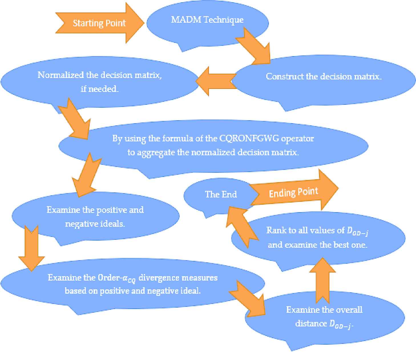
Geometrical interpretation of the explored algorithm.
Example 1.
With the improvement of internet business stages, web-based shopping has become a typical utilization propensity for buyers. A customer plans to purchase a cell phone on a web-based business stage. The mobile phones are considered as alternatives, whose representations are followed as
For alternatives
Step 1: By using Eq. (42), we construct the decision matrix, whose entries in the form of CQRONFNs.
Step 2: By using Eq. (43), we normalize the decision matrix, which is given in step 1, if needed. The matrix, which is mention in the Table 1 is not needed to normalize it.
| Symbols | ||||
|---|---|---|---|---|
Original decision matrix, whose every entry in the form of complex q-rung orthopair normal fuzzy numbers.
Step 3: By using Eq. (41), we aggregate the values, which are normalized in step 2, for
Step 4: By using Eqs. (44) and (45), we evaluate the positive and negative ideas, such that
Step 5: By using the Eq. (28), we examine the Order-
Step 6: By using Eq. (46), we examine the overall distance measure based on the
Step 7: Rank all alternatives, which we get in step 6 and we examine the best alternative from the family of alternatives, such that
The best alternative is
Step 8: The end.
6.1. Comparative Analysis
Keeping the advantages of the explored notions is called CQRONFSs and their AOs, we solve some numerical examples to examine the reliability and effectiveness of the presented work. For coping with such kind of issues, we considered different kinds of information and resolved it by using explored and existing operators, whose information's are discussed below.
Additionally, the compassion among presented work and existing works are discussed to observe the proficiency and expertise of the explored approach. The existing technique of intuitionistic normal fuzzy AOs was proposed by Wang and Li [30], and the q-rung orthopair normal fuzzy AOs were presented by Yang et al. [31].
From the above analysis, it is clear that the existing approaches [30,31] and explored approach in these manuscripts give the same ranking results, which is in the form of
| Symbols | ||
|---|---|---|
By using Eq. (28), we examine the distance measures based on positive and negative ideals.
| Methods | Operators | Score Values | Ranking |
|---|---|---|---|
| Wang and Li [30] | WA | ||
| WG | |||
| GWA | |||
| GWG | |||
| Yang et al. [31] | WA | ||
| WG | |||
| GWA | |||
| GWG | |||
| Proposed method for q = 1 | WA | ||
| WG | |||
| GWA | |||
| GWG | |||
| Proposed method for q = 2 | WA | ||
| WG | |||
| GWA | |||
| GWG | |||
| Proposed method for q = 3 | WA | ||
| WG | |||
| GWA | |||
| GWG |
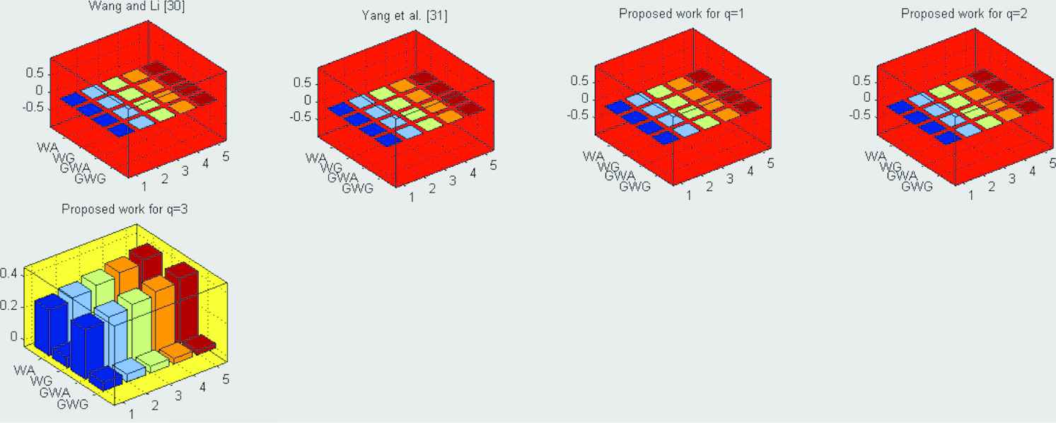
Comparison between explored work with some existing operators.
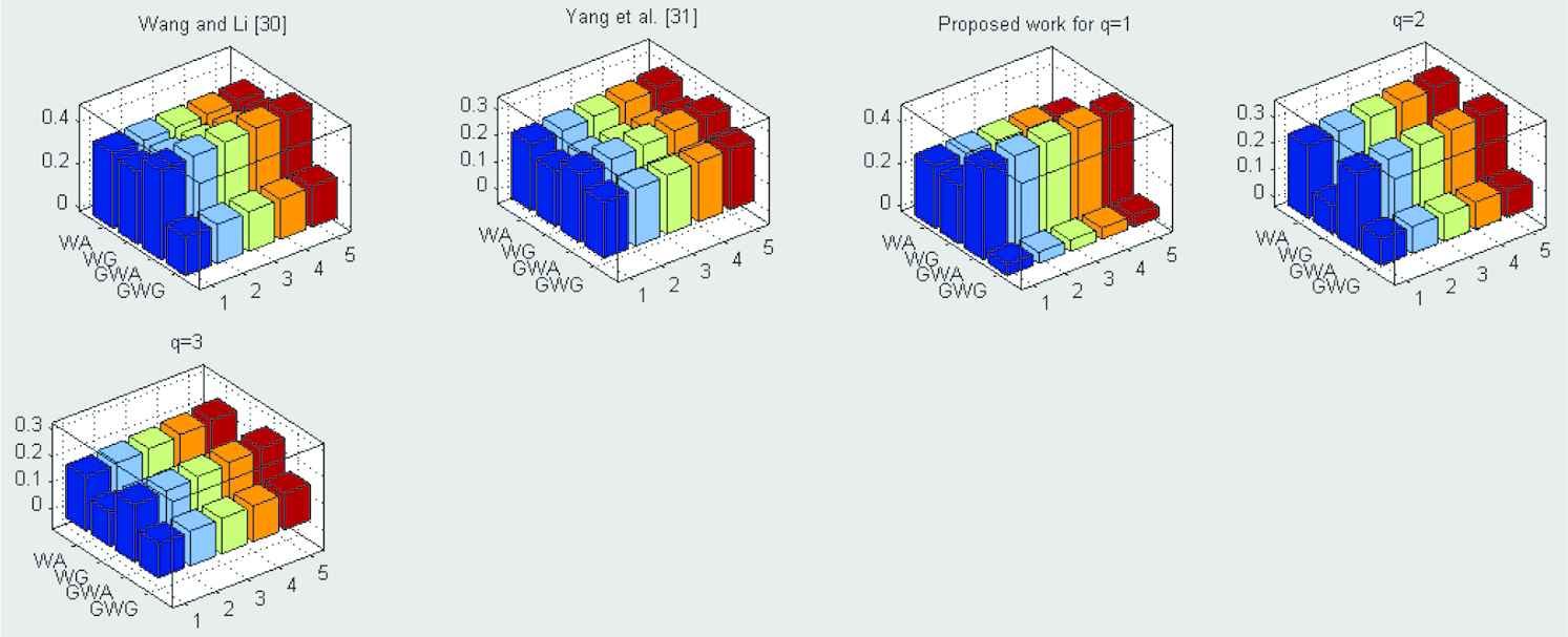
Geometrical representation for the informations of Table 4.
| Symbols | ||||
|---|---|---|---|---|
Original decision matrix, whose information in the form of complex Pythagorean normal fuzzy numbers.
From Table 2 we considered the complex intuitionistic normal fuzzy information and resolved it by using the explored and existing operators [30,31] to examine the proficiency and expertise of the presented approach. Further, to find the reliability of the explored operator, we choose the complex Pythagorean normal fuzzy information and solve it by using the explored and existing operators [30,31].
Form Figure 3 there are mentions five kinds of series, which are denoted the graph of alternatives in different colors. From Figure 3, we easily obtained that which one is the best alternative, see the above figure the series five is moved on the top in all series, so series five is the best alternative from the set of alternatives. The information's are discussed in Table 5 for
| Methods | Operators | Score Values | Ranking |
|---|---|---|---|
| Wang and Li [30] | WA | Failed | Failed |
| WG | Failed | Failed | |
| GWA | Failed | Failed | |
| GWG | Failed | Failed | |
| Yang et al. [31] | WA | ||
| WG | |||
| GWA | |||
| GWG | |||
| Proposed method for q = 1 | WA | Failed | Failed |
| WG | Failed | Failed | |
| GWA | Failed | Failed | |
| GWG | Failed | Failed | |
| Proposed method for q = 2 | WA | ||
| WG | |||
| GWA | |||
| GWG | |||
| Proposed method for q = 3 | WA | ||
| WG | |||
| Proposed method for q = 3 | GWA | ||
| GWG |
Comparison between explored work with some existing operators.
Based on the explored operators are called WA, WG, GWA, GWG operators based on complex Pythagorean normal fuzzy information's, the compassion among presented work and existing works are discussed to observe the proficiency and expertise of the explored approach. The existing technique of intuitionistic normal fuzzy AOs was proposed by Wang and Li [30], and the q-rung orthopair normal fuzzy AOs were presented by Yang et al. [31]. The aggregated values for proposed work and existing works are illustrated in Table 6.
| Symbols | ||||
|---|---|---|---|---|
Original decision matrix, whose information in the form of complex q-rung orthopair normal fuzzy numbers.
From the above analysis, it is clear that the existing approaches [30,31] and explored approach in this manuscripts give the different ranking results, which are in the form of
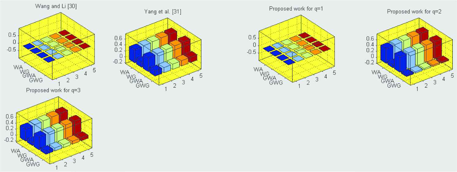
Geometrical representation for the informations of Table 6.
Form Figure 4 there are mentions five kinds of series, which are denoted the graph of alternatives in different colors. From Figure 4, we easily obtained that which one is the best alternative, see the above figure the series five is moved on the top in all series, so series five is the best alternative from the set of alternatives. From Tables 1 and 5 we considered the complex intuitionistic normal fuzzy information, complex Pythagorean normal fuzzy information and resolved it by using the explored and existing operators [30,31] to examine the proficiency and expertise of the presented approach. Further, to find the reliability of the explored operator, we choose the complex q-rung orthopair normal fuzzy information and solve it by using the explored and existing operators [30,31]. The information is discussed in Table 7.
| Methods | Operators | Score Values | Ranking |
|---|---|---|---|
| Wang and Li [30] | WA | Failed | Failed |
| WG | Failed | Failed | |
| GWA | Failed | Failed | |
| GWG | Failed | Failed | |
| Yang et al. [31] | WA | Failed | Failed |
| WG | Failed | Failed | |
| GWA | Failed | Failed | |
| GWG | Failed | Failed | |
| Proposed method for q=1 | WA | Failed | Failed |
| WG | Failed | Failed | |
| GWA | Failed | Failed | |
| GWG | Failed | Failed | |
| Proposed method for q = 2 | WA | Failed | Failed |
| WG | Failed | Failed | |
| GWA | Failed | Failed | |
| GWG | Failed | Failed | |
| Proposed method for q = 8 | WA | ||
| WG | |||
| GWA | |||
| GWG |
Comparison between explored work with some existing operators.
Based on the explored operators are called WA, WG, GWA, GWG operators based on complex Pythagorean normal fuzzy information's, the compassion among presented work and existing works are discussed to observe the proficiency and expertise of the explored approach. The existing technique of intuitionistic normal fuzzy AOs was proposed by Wang and Li [30], and the q-rung orthopair normal fuzzy AOs were presented by Yang et al. [31]. The aggregated values for proposed work and existing works are illustrated in Table 8.
| Symbols | ||||
|---|---|---|---|---|
Original decision matrix.
From the above analysis, it is clear that the existing approaches [30,31] and explored approach in this manuscripts give different ranking results, which are in the form of
Geometrical representation for the informations of Table 8.
Form Figure 5 there are mentions five kinds of series, which are denoted the graph of alternatives in different colors. From Figure 5, we easily obtained that which one is the best alternative, see the above figure the series five is moved on the top in all series, so series five is the best alternative from the set of alternatives. Further, we examine the reliability and proficiency of the explored measures and operators based on CQRONFSs. We illustrate a numerical example which is discussed below is taken from Ref. [31].
Example 2.
As economic globalization makes enterprises face a more complex internal and external environment, finding an appropriate partner is an important way to maintain their competitiveness, which is affected by many factors. To select a suitable global partner, an enterprise has selected five candidate enterprises in the global scope. The set of alternative enterprises is
Based on the explored operators are called WA, WG, GWA, GWG operators based on complex Pythagorean normal fuzzy information's, the compassion among presented work and existing works are discussed to observe the proficiency and expertise of the explored approach. The existing technique of intuitionistic normal fuzzy AOs was proposed by Wang and Li [30], and the q-rung orthopair normal fuzzy AOs were presented by Yang et al. [31]. The aggregated values for proposed work and existing works are illustrated in Table 9.
| Methods | Operators | Score Values | Ranking |
|---|---|---|---|
| Wang and Li [30] | WA | Failed | Failed |
| WG | Failed | Failed | |
| GWA | Failed | Failed | |
| GWG | Failed | Failed | |
| Yang et al. [31] | WA | ||
| WG | |||
| GWA | |||
| GWG | |||
| Proposed method for q = 1 | WA | Failed | Failed |
| WG | Failed | Failed | |
| GWA | Failed | Failed | |
| GWG | Failed | Failed | |
| Proposed method for q = 2 | WA | Failed | Failed |
| WG | Failed | Failed | |
| GWA | Failed | Failed | |
| GWG | Failed | Failed | |
| Proposed method for q = 8 | WA | ||
| WG | |||
| GWA | |||
| GWG |
Comparison between explored work with some existing operators.
From the above analysis, the ranking results of the proposed and existing notions are the same which is in the form of
Original decision matrix.
Based on the explored operators are called WA, WG, GWA, GWG operators based on complex Pythagorean normal fuzzy information's, the compassion among presented work and existing works are discussed to observe the proficiency and expertise of the explored approach. The existing technique of intuitionistic normal fuzzy AOs was proposed by Wang and Li [30], and the q-rung orthopair normal fuzzy AOs were presented by Yang et al. [31]. The aggregated values for proposed work and existing works are illustrated in Table 11.
| Methods | Operators | Score Values | Ranking |
|---|---|---|---|
| Wang and Li [30] | WA | ||
| WG | |||
| GWA | |||
| GWG | |||
| Yang et al. [31] | WA | ||
| WG | |||
| GWA | |||
| GWG | |||
| Proposed method for q = 1 | WA | ||
| WG | |||
| GWA | |||
| GWG | |||
| Proposed method for q = 2 | WA | ||
| WG | |||
| GWA | |||
| GWG | |||
| Proposed method for q = 3 | WA | ||
| WG | |||
| GWA | |||
| GWG |
Comparison between explored works with some existing operators.
From the above analysis, the ranking results of the proposed and existing notions are the same which is in the form of
| Parameter | Score Values | Ranking Values |
|---|---|---|
Discussed for different values of the parameter
Therefore, the explored operators based on CQRONFSs are more proficient and more flexible than existing operators, which is discussed in Ref. [30,31]. Hence, the presented approach is extensively powerful and more general than complex intuitionistic normal fuzzy setFSs and complex Pythagorean normal FSs.
7. CONCLUSION
One of the most proficient and beneficial theories is called CQROFS, containing the grade of supporting and the grade of supporting against in the form of polar coordinates belonging to unit disc in a complex plane. CQROFS is a proficient technique to address awkward information, although the NFN is examining normal distribution information in anthropogenic action and realistic environment. Based on the advantages of both notions, in this manuscript, we explored the novel concept of CQRONFS as an important technique to evaluate unreliable and complicated information. Some operational laws based on CQRONFSs are also explored. Additionally, some distance measures are called CQRONFGDM, CQROFNFSDM, two types of CQRONFODMs, and their special cases are discussed. Moreover, weighted averaging, weighted geometric, generalized weighted averaging, and generalized weighted geometric operators based on CQRONFSs are also presented. In last, we solve a numerical example of the MADM problem is shown to justify the proficiency of the presented operators. The advantages, comparative and sensitive analysis are used to express the efficiency and flexibility of the explored approach.
In further research, considering the superiority of new CQRONFSs, we can extend them to some other work based on FSs [32,33], picture FSs [34], PFSs [35], hesitant fuzzy setFSs [36], and so on [37–42].
CONFLICTS OF INTEREST
The authors declare no conflict of interest.
AUTHORS’ CONTRIBUTIONS
All authors have equally contributed to this manuscript.
ACKNOWLEDGMENTS
The authors are grateful to the Deanship of Scientific Research, King Saud University for funding through Vice Deanship of Scientific Research Chairs.
REFERENCES
Cite this article
TY  - JOUR
AU  - Zeeshan Ali
AU  - Tahir Mahmood
AU  - Abdu Gumaei
PY  - 2021
DA  - 2021/07/01
TI  - Order-αCQ Divergence Measures and Aggregation Operators Based on Complex q-Rung Orthopair Normal Fuzzy Sets and Their Application to Multi-Attribute Decision-Making
JO  - International Journal of Computational Intelligence Systems
SP  - 1895
EP  - 1922
VL  - 14
IS  - 1
SN  - 1875-6883
UR  - https://doi.org/10.2991/ijcis.d.210622.004
DO  - 10.2991/ijcis.d.210622.004
ID  - Ali2021
ER  -