
Continuous Prediction of the Gas Dew Point Temperature for the Prevention of the Foaming Phenomenon in Acid Gas Removal Units Using Artificial Intelligence Models
- DOI
- 10.2991/ijcis.2017.10.1.12How to use a DOI?
- Keywords
- Foaming; Acid Gas Removal; Artificial Neural Network; Imperialist Competitive Algorithm; Particle Swarm Optimization
- Abstract
Acid gas removal (AGR) units are widely used to remove CO2 and H2S from sour gas streams in natural gas processing. When foaming occurs in an AGR system, the efficiency of the process extremely decreases. In this paper, a novel approach is suggested to regularly predict the gas dew point temperature (GDPT) in order to anticipate the foaming conditions. Prediction of GDPT is advantageous because the conventional methods of measuring GDPT such as: (i) using a chilled mirror device is time consuming; and (ii) the use of gas chromatograph for composition determination combined with the equation-of-state calculations involve column retention time and is expensive. New hybrid modeling algorithms based on the artificial neural network (ANN) combined with either the imperialist competitive algorithm (ICA) or particle swarm optimization (PSO) are employed to model the process. The models can then be used to prevent the foaming phenomenon. The proposed algorithms combine the local searching ability of ANN with the global searching abilities of ICA and PSO. ICA and PSO are used to optimize the initial weights of the neural networks. The resulting ICA-ANN and PSO-ANN combined algorithms are then applied to model the occurrence of foaming in the AGR plant based on a simulation data set acquired from the 6th refinery of the south Pars gas complex in Iran. The performances of the ICA-ANN, PSO-ANN and conventional ANN models are then compared against each other. It was found that the accuracies of the ICA-ANN and PSO-ANN models are better than that of the conventional ANN model. In addition, the PSO-ANN model outperformed the ICA-ANN model.
- Copyright
- © 2017, the Authors. Published by Atlantis Press.
- Open Access
- This is an open access article under the CC BY-NC license (http://creativecommons.org/licences/by-nc/4.0/).
1. Introduction
AGR units are used to remove CO2 and H2S from sour gas in natural gas processing. When foaming occurs in an AGR system, the efficiency of the acid gas removal process extremely decreases. One of the principle causes of foaming is the formation of liquid hydrocarbons in the process. Liquid hydrocarbons are highly soluble in the amine solution and reduce the surface tension of the solution. The reduced surface tension then results in foaming. Determining the dew point of the inlet gas provides the opportunity to avoid liquid hydrocarbons entering the process1.
ANN is a tool widely used in modeling and control problems. The most important factor in utilizing ANN is the determinations of its network structure and parameters. Evolutionary algorithms such as ICA2 and PSO3, 4 can be employed to achieve these objectives. ICA and PSO5–7 are evolutionary optimization methods which have shown great performance in the global optimum achievement. In the present work, ICA and PSO are employed to optimize the initial weights of ANN. The simulation results demonstrated the effectiveness and potential of the newly proposed ICA-ANN and PSO-ANN for modeling and prediction of the foaming conditions in the 6th refinery of the south Pars gas complex. The performances of the resulting models and the conventional neural network model are then compared against each other utilizing the same data set.
2. Acid Gas Removal and Foaming
Natural gas contains toxic components such as CO2 and H2S and must be treated in natural gas refineries before being utilized. The acid gas removal process, also known as the gas sweetening process, widely uses amines as solvent to treat the sour gas. The amine solution and sour gas are contacted in an absorber column to remove the acid gas. A typical absorber column is illustrated in Fig. 1.
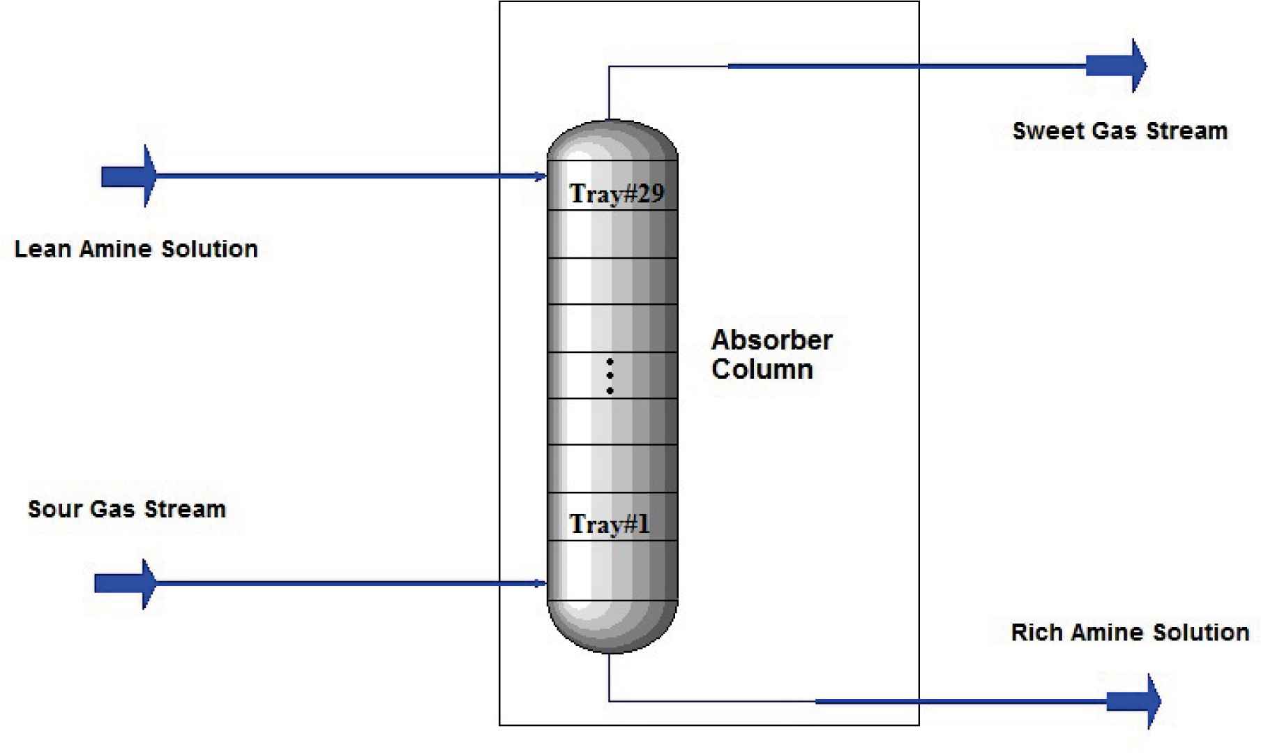
Schematic of a typical absorber column.
As shown in this figure, the sour gas stream enters the bottom of the absorber and is contacted to the lean amine solution entered from the top. The lean amine absorbs the acid gas and leaves the bottom of column as rich amine. On the other side, the sour gas passes the height of column and leaves the top of the column as sweet gas (containing no acid gas).
Foaming is an undesirable phenomenon and needs to be prevented. Foam is the result of confinement of a volume of gas into a liquid. The liquid film surrounds the gas and creates a bubble. The foaming tendency of a liquid is indicated by a parameter called the surface tension (g). The surface tension is a force which acts parallel to the liquid surface and opposes the expansion of its surface area (A). The work required to expand the surface area is called the surface free energy (G) which depends on the cohesive and intermolecular forces in the liquid. The incremental values of the variables G and A are related by:
For liquid surface expansion, molecules must move from the interior of the liquid to the surface. Liquids with a low surface tension require less energy to expand their surfaces and tend to foam easily; therefore the lower the surface tension the more will be their tendency to create foam.
Like any liquid, the amine solutions could also foam. Foaming in amine plants is an undesirable common phenomenon which reduces the efficiency of the plant. When foaming becomes severe, amine is often carried over from the top of absorber and causes upset8.
Pure amines have a polar structure in which strong intermolecular forces lead to a high surface tension; therefore they do not form stable foams. When one or more components are present in the amine solution as impurities, its foaming tendency greatly increases.
The primary cause of foaming problems has been considered to be due to the existence of liquid hydrocarbons in the amine solutions. Liquid hydrocarbons have a non-polar and weak structure and therefore will reduce the surface tension of the amine solution and increase its tendency to foam. In fact, avoiding entrance of liquid hydrocarbons into the amine solutions makes it possible to prevent the foaming problems in the AGR plants8.
3. The Novel Proposed Technique: Dew Point Monitoring
As mentioned before, the principle reason of the amine foaming is the formation of liquid hydrocarbons in the amine absorber.
When liquid hydrocarbons form in the gas stream in the absorber, they are highly soluble into the amine solution and reduce its surface tension. The reduced surface tension then aids in foaming.
Dew point temperature of a gas in a constant pressure is defined as the temperature at which the components of gas start to condense and form a liquid phase. In order to prevent the creation of the liquid hydrocarbons in the gas stream, the temperature of the gas in the absorber must not be lower than its dew point temperature.
In this work, a novel approach in which two temperatures are to be regularly monitored to avoid foaming is suggested: (i) GDPT at the absorber pressure; and (ii) the gas temperature in the absorber.
Fig. 2 illustrates the concept of the suggested approach. As shown in this figure, when the gas temperature is above GDPT, the flowing stream is a single phase gas and there is no risk of foaming; but when it approaches and equals GDPT, the heavier components of gas begin to drop out into the liquid phase, increasing the risk of foaming in the amine absorber. If the temperature is below GDPT, the gas stream no longer is in the gas phase and has a two-phase flow which means liquid hydrocarbons are entered into the absorber and the foaming is imminent.
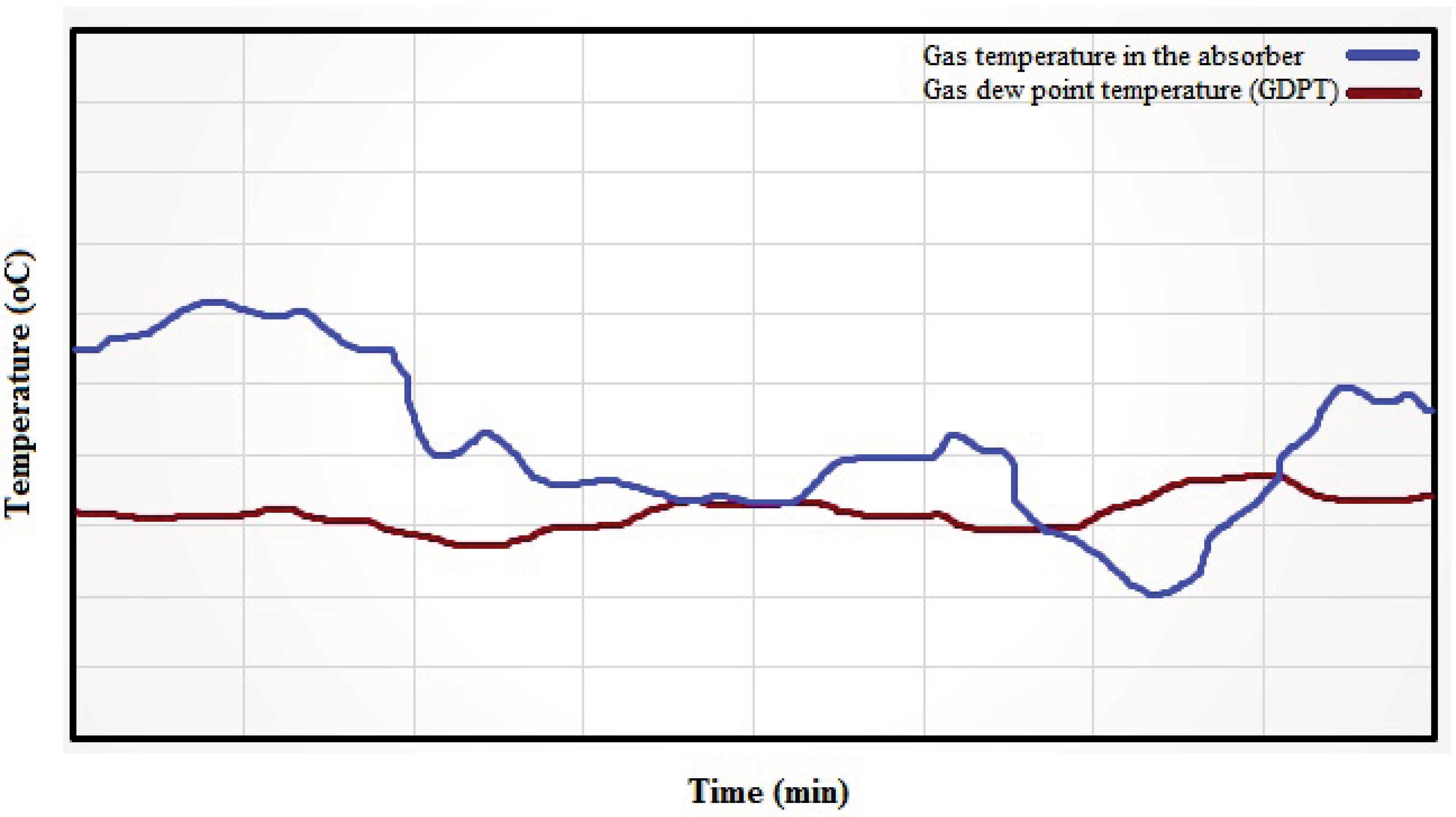
Typical illustration of the proposed temperature monitoring approach for the detection of foaming.
The suggested GDPT monitoring approach could be modeled by a robust modeling tool which will be utilized to prevent foaming of the AGR plant.
4. Artificial Neural Network
ANN is a modeling tool composed of elements inspired by human nervous systems. ANNs are structured from simple units called neurons representing processing cells in human brain. Neurons are connected together by weighted connections. ANNs are able to express non-linear relationships using experimental input-output data. A simplified procedure of training an ANN is shown in Fig. 3. In network training, an input leads to a specific output; then the output is compared to a given target and based on the comparison, the network elements (weights) are adjusted until the network output matches the target9.

Simplified procedure of the network training.
The approximation capabilities of the multilayer perceptron (MLP) architecture make it a popular choice for modeling cases employed by chemical, petroleum and natural gas engineers10. MLPs are composed of the input layer, hidden layer(s) and output layer.
A typical three layer MLP network may consists of I neurons in the input layer, J neurons in the hidden layer, and K neurons in the output layer.
The number of independent input parameters affecting the target parameter(s) specifies the number of neurons in the input layer and number of target parameter(s) defines the number of the output layer neurons. Commonly, the optimum number of neurons in the hidden layer(s) is determined by a trial and error procedure. The privilege of the MLP network is its ability to express non-linear functions. Activation transfer functions like threshold, log-sigmoid, and tan-sigmoid could be employed to incorporate non-linearity into MLPs.
To adjust the values of weights of the network in order to train the MLP network, a proper learning algorithm should be utilized. The back propagation (BP) training algorithm is one of the most commonly used algorithms due to its high performance in lowering the generated error11. In a feed-forward neural network which utilizes the BP algorithm, a set of input data is introduced to the network and the outputs are estimated by the network. In the next step, the difference between the actual and the estimated output values, i.e. error, is calculated and the network starts going backward to adjust the weights. When all the weights are updated, the network returns back to the forward propagation to estimate the new output for the network. Error calculation and weight adjustment steps continue until the generated error reaches a minimum12.
A three layered feed-forward neural network employing the BP algorithm can estimate any non-linear function to an arbitrary accuracy.
The BP algorithm uses the gradient descent method to minimize the error and is vulnerable to get trapped into a local minimum, making it entirely dependent on its initial settings (weights). This problem can be alleviated by the global searching ability of an evolutionary algorithm such as PSO13.
5. Imperialist Competitive Algorithm
ICA14–17 is a new global search strategy that has lately been introduced for dealing with different optimization obligations. ICA can be used to design an optimal controller or find the optimized weights of ANNs18. Like other evolutionary algorithms, ICA commences with an initial population of P countries produced accidentally within an achievable space. The best Nimp number of countries in the initial population, considering the cost functions of them, are chosen as the imperialists and other countries are taken as the colonies of these imperialists. To construct the initial empires, colonies are apportioned among the imperialists based on the power of each imperialist. To distribute the colonies among the imperialists proportionally, the following normalized cost of an imperialist is defined:
After dividing colonies among imperialists, a colony moves toward its relevant imperialist.
The entire power of an empire can be equal to the power of the imperialist country plus a percentage of the power of its colonies as:
After starting competition, any empire that cannot succeed in this competition and cannot increase its power will be removed from the competition. The results of competition will be an increase in the powers of the robust empires and a decrease in the powers of weak ones. At the end, by using the movement of colonies toward their related imperialists, one empire will emerge as the answer of optimization problem. The optimization steps of ICA are as follows10:
- (i)
Select some random points and initialize the empires.
- (ii)
Move the colonies towards their relevant imperialists (assimilation).
- (iii)
Randomly change the position of some colonies (revolution).
- (iv)
If there is a colony in an empire which has a lower cost than the imperialist, change the positions of that colony and the imperialist.
- (v)
Unite the similar empires.
- (vi)
Compute the total cost of all empires.
- (vii)
Separate the weakest colony (colonies) from the weakest empires and give it (them) to one of the empires (imperialistic competition).
- (viii)
Destroy the powerless empires.
- (ix)
If the stop conditions (maximum number of iterations or a sufficiently low mean square error (MSE) value are satisfied, then stop, if not go to step (ii).
6. Particle Swarm Optimization
The PSO Algorithm was first proposed by Kennedy and Eberhart19 and has proven to be a powerful tool for global optimization problems. PSO is inspired by social behavior of bird or fish crowd and is interesting due to its small number of parameters required to be tuned. Furthermore, PSO has simple procedure which could be summarized by the following steps:
- (i)
Initialize the swarm by assigning a random position in the parameter space to each particle with a rational random velocity.
- (ii)
Evaluate the fitness function for each particle.
- (iii)
For each individual particle, compare the particle’s fitness value with its personal best position (pbest). If the current value is better than the pbest value, then the pbest value and the corresponding position are replaced by the current fitness value and position, respectively.
- (iv)
Update the global best fitness value and the corresponding best position.
- (v)
Update the velocities and positions of all the particles.
- (vi)
Repeat steps (ii) to (v) until a stopping criterion (maximum number of iterations or a sufficiently low MSE value) is encountered.
7. Model Development
The purpose of the present study is to develop ANN-based models using ICA and PSO to estimate the conditions of the foaming phenomenon in an absorber column of a gas sweetening plant. The two optimization algorithms ICA and PSO are used for the ANN training and the results are then compared to the corresponding simple ANN model. The parameters corresponding to the PSO and ICA algorithms utilized in this work are tabulated in Table 1.
| PSO parameters | ICA parameters | ||
|---|---|---|---|
| Population size | 80 | Population size | 80 |
| Initial inertia weight | 0.2 | Initial empires | 8 |
| Final inertia weight | 0.9 | Initial colonies | 72 |
| Cognitive parameter c1 | 1.2 | Movement parameter β | 2.1 |
| Social parameter c2 | 2.8 | Direction deviation parameter γ | π/4 (rad) |
Parameters of PSO and ICA.
To develop the network, data were collected from the dynamic plant simulation relevant to the 6th refinery of the south Pars gas complex in Iran. A simulation package known as the DYNAMIC20 is utilized to simulate the dynamic behavior of the absorber column.
In the developed model, GDPT is predicted. GDPT is a function of the temperature of sour gas (TSG) stream, temperature of lean amine (TLA), the flow of lean amine (FLA), and the pressure of sour gas (PSG).
Random step change signals were imposed on TSG, TLA, FLA, and PSG as the model inputs and the variations of GDPT were recorded as the model output. The simulation data collection time lasted for 2000 minutes and the data were recorded every 2 minutes. A white Gaussian noise with 5% variance of the magnitude of GDPT was also added to the datasets. This is performed in order to obtain a more realistic measured data.
The operating ranges of the collected dataset are given in Table 2. The datasets of input variables of the model: FLA, TLA, TSG, and PSG are correspondingly shown in Figs. 4(a), 4(b), 4(c), and 4(d). The variable GDPT (output dataset of the model) is depicted in Fig. 4(e).
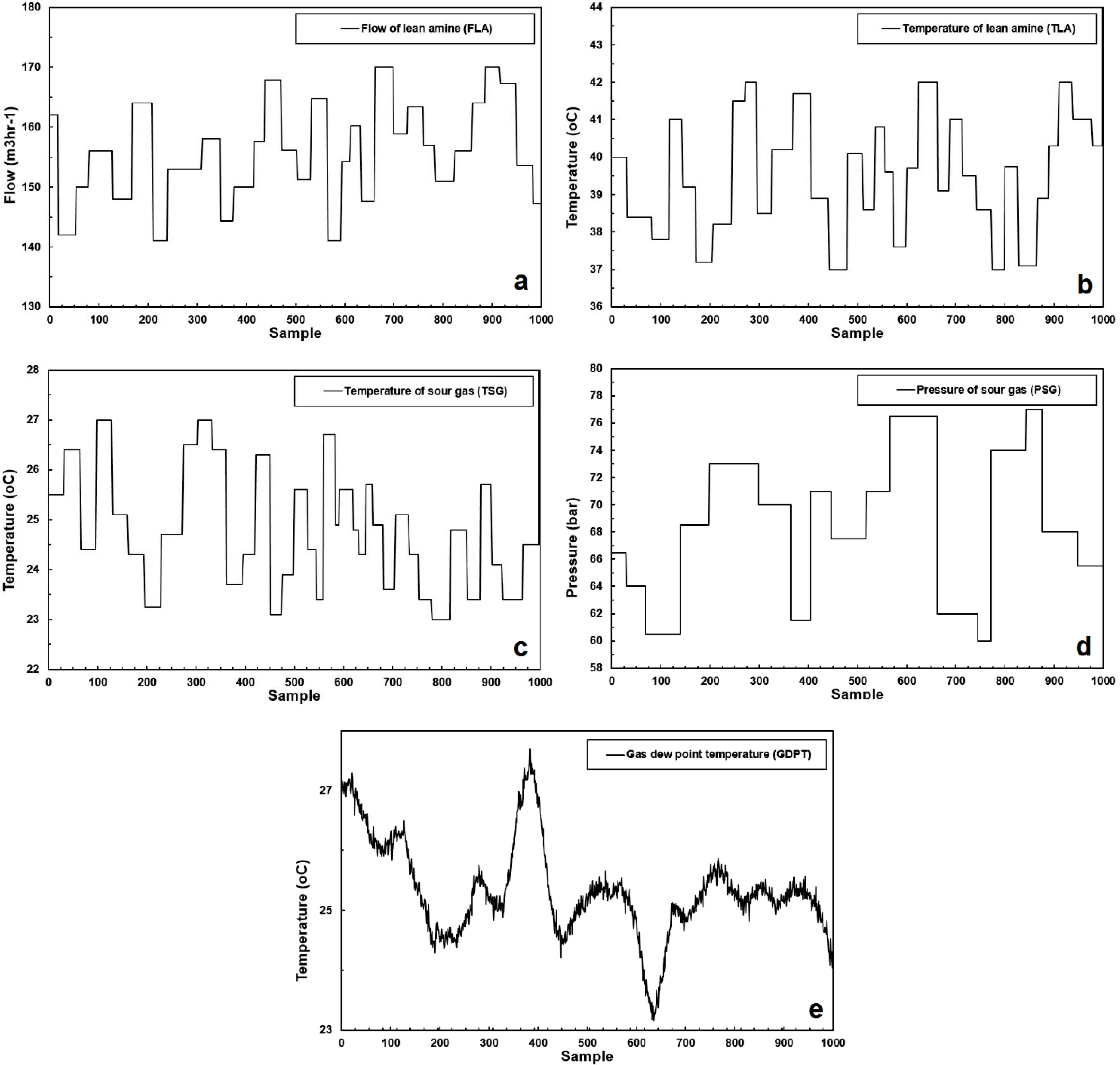
(a) Flow of the lean amine; (b) temperature of the lean amine; (c) temperature of the sour gas stream; (d) pressure of the sour gas stream; and (e) the gas dew point temperature.
| Parameter | Min. | Max. |
|---|---|---|
| TSG (°C) | 23 | 27 |
| FLA (m3hr−1) | 140 | 170 |
| TLA (°C) | 37 | 42 |
| PSG (bar) | 60 | 77 |
The operating ranges of the collected dataset employed to estimate GDPT.
To express the dynamic behavior of the model, a first order lag is utilized. Therefore the model can be written as:
Before developing the models, all the collected input data points were normalized between zero and one as the preprocessing step using the following equation:
In the next step the normalized dataset were divided into three sub-datasets including the training data (70%), validation data (15%), and test data (15%). The training sub-dataset is used to tune the weights of the network and train the model. The validation sub-dataset is employed to avoid over-fitting. The test set is utilized to evaluate the estimation ability of the model.
To determine the best structure for the network there is no unique procedure; therefore trial and error is performed. In this study, the best network topology is chosen based on the correlation coefficient (R-squared) and the MSE criteria. A BP ANN with a single hidden layer is employed to develop the model. The network is trained by the Levenberge Marquardt (LM) technique and the tan-sigmoid and linear transfer functions have been assigned to the hidden and output layers, respectively. The number of hidden neurons is selected to be equal to seven. This is achieved by changing the hidden neurons from three to ten, training the resulting networks using the train and validation data sets and testing the resulting networks using the test data set. Consequently, the network with the number of hidden neurons equal to seven resulted in a minimum MSE for the test data set. Therefore, considering equation 5, the best topology for the model will be 8-7-1. Model verification is the final and the most important step in the model development. In this study, the R-squared and MSE are chosen as the criteria for the accuracy determination of the model. The model becomes accurate as the R-squared and MSE approach to 1 and 0, respectively.
The R-squared and MSE are correspondingly defined by the following two equations:
In these two equations, n is the number of data points, yi is the actual value of GDPT, ye is the estimated value of GDPT, and ya is the average value of the plant data.
The stopping criteria for the ANN models are considered as either the MSE value being equal to 1e-8 or the maximum number of iterations becomes equal to 500.
8. Results and Discussion
The predicted output and the measured data for GDPT are given in Figs. 5(a), 5(b), and 5(c) for the ANN, ICA-ANN, and PSO-ANN models, respectively.
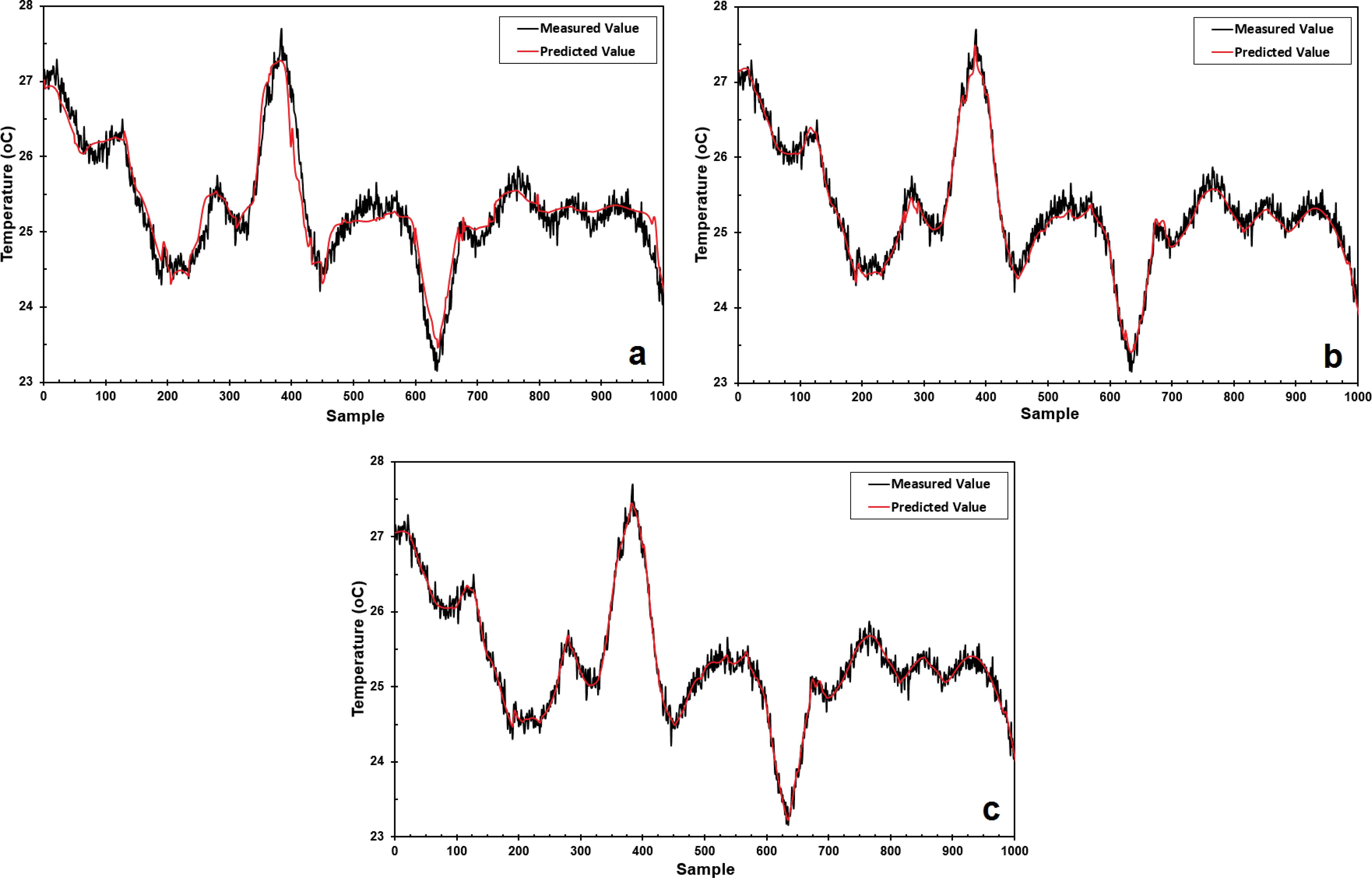
(a) The predicted output and the measured data of the GDPT for the: (a) ANN model; (b) ICA-ANN model; and (c) PSO-ANN model.
Figs. 6(a), 6(b), and 6(c) depict the parity plots of the train dataset for the outputs predicted by the models against the measured plant data, for the ANN, ICA-ANN, and PSO-ANN models, respectively. Figs. 7(a), 7(b), and 7(c) show the parity plots of the test dataset for the outputs predicted by the models against the measured data, for the ANN, ICA-ANN, and PSO-ANN models, respectively. The performances of the developed models with regard to their MSE values versus epochs are graphically shown in Figs. 8(a), 8(b), and 8(c) for the ANN, ICA-ANN, and PSO-ANN models, respectively. The circles in these figures indicate the iterations beyond which no appreciable performance improvements are resulted and the performances may well deteriorate on the validation data sets.
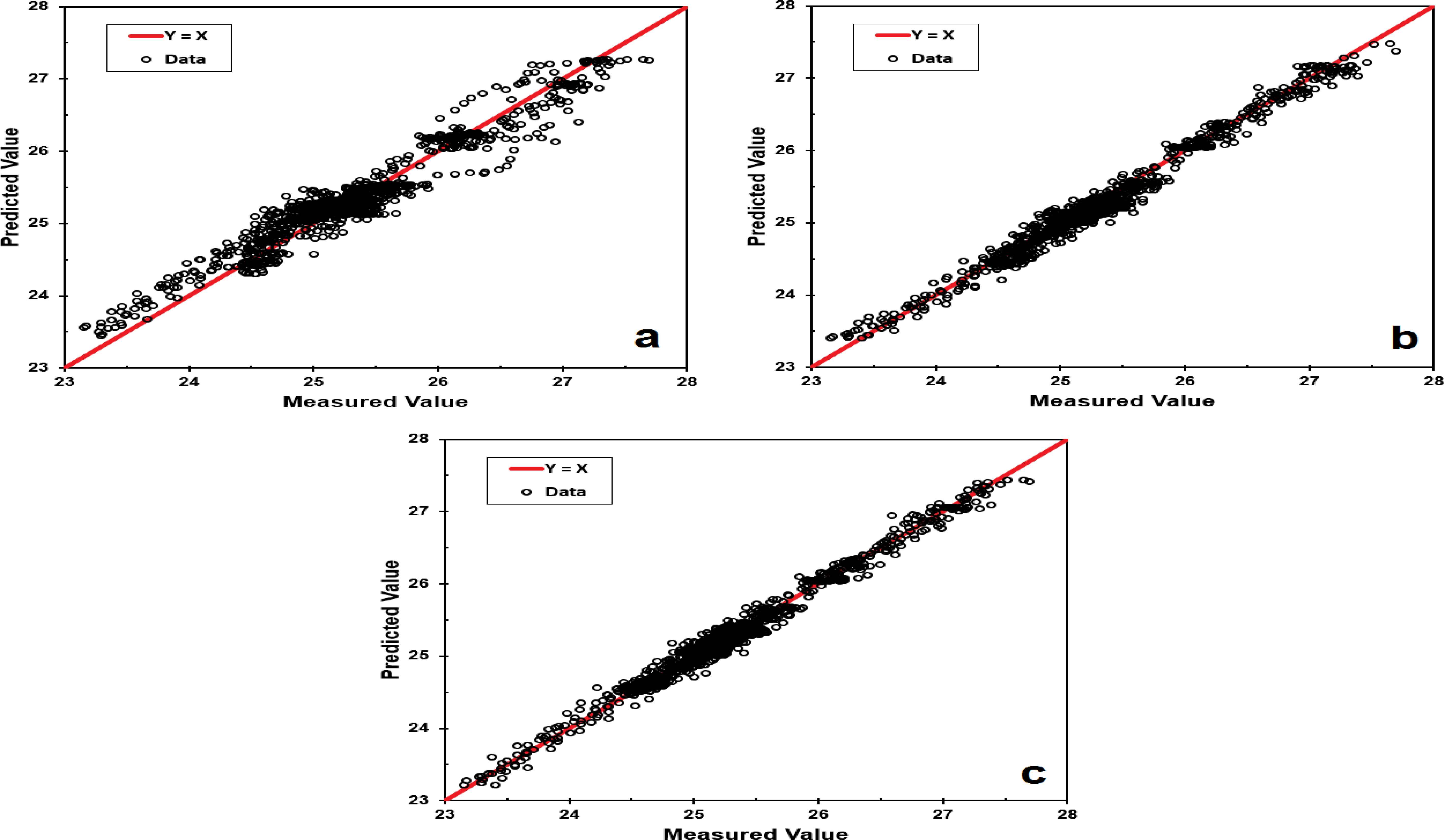
Parity plots of the train dataset for the outputs predicted by the models against the measured data: (a) ANN model; (b) ICA-ANN model; and (c) PSO-ANN model.
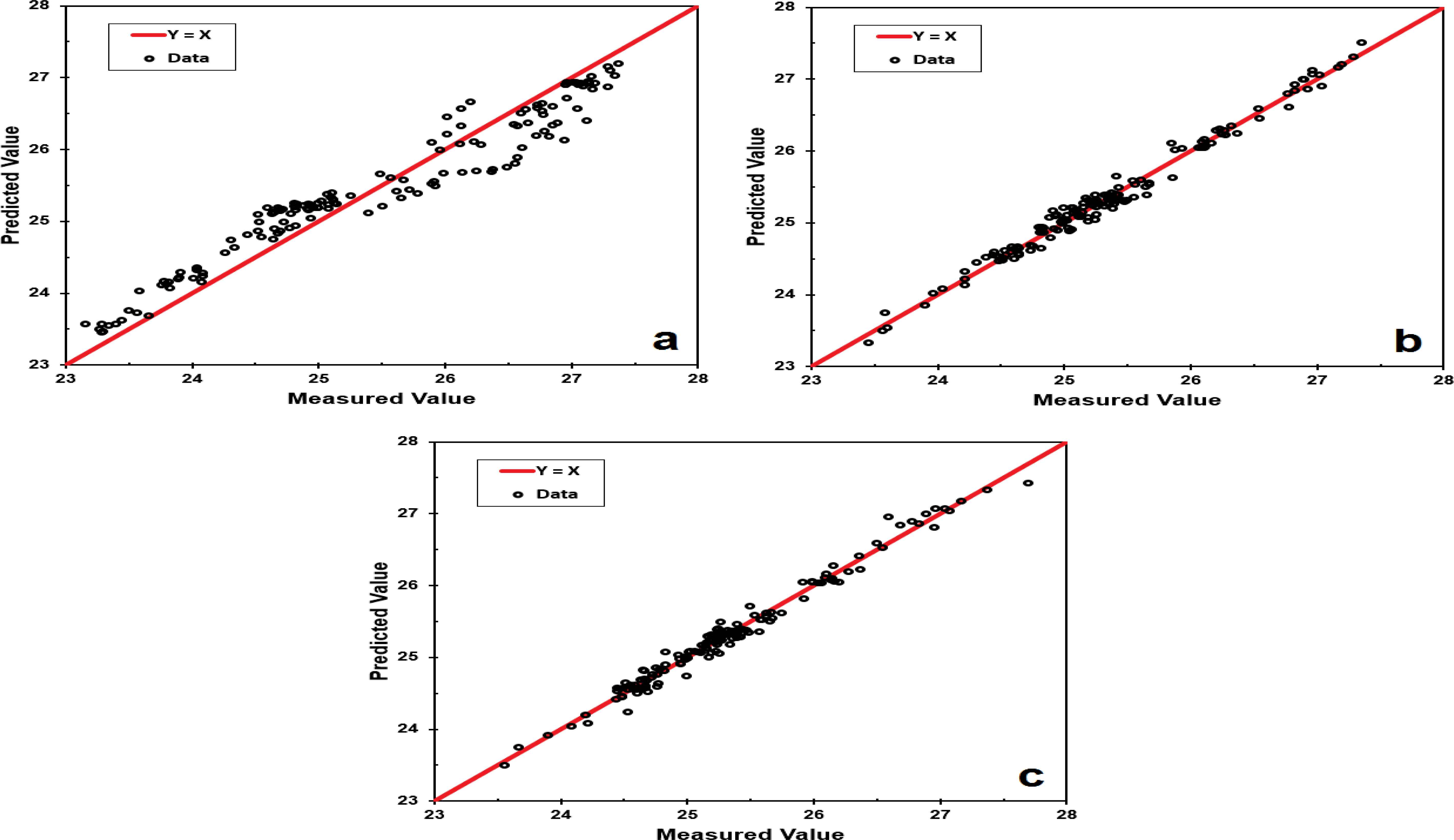
Parity plots of the test dataset for the outputs predicted by the models against the measured data: (a) ANN model; ICA-ANN model; and (c) PSO-ANN model.
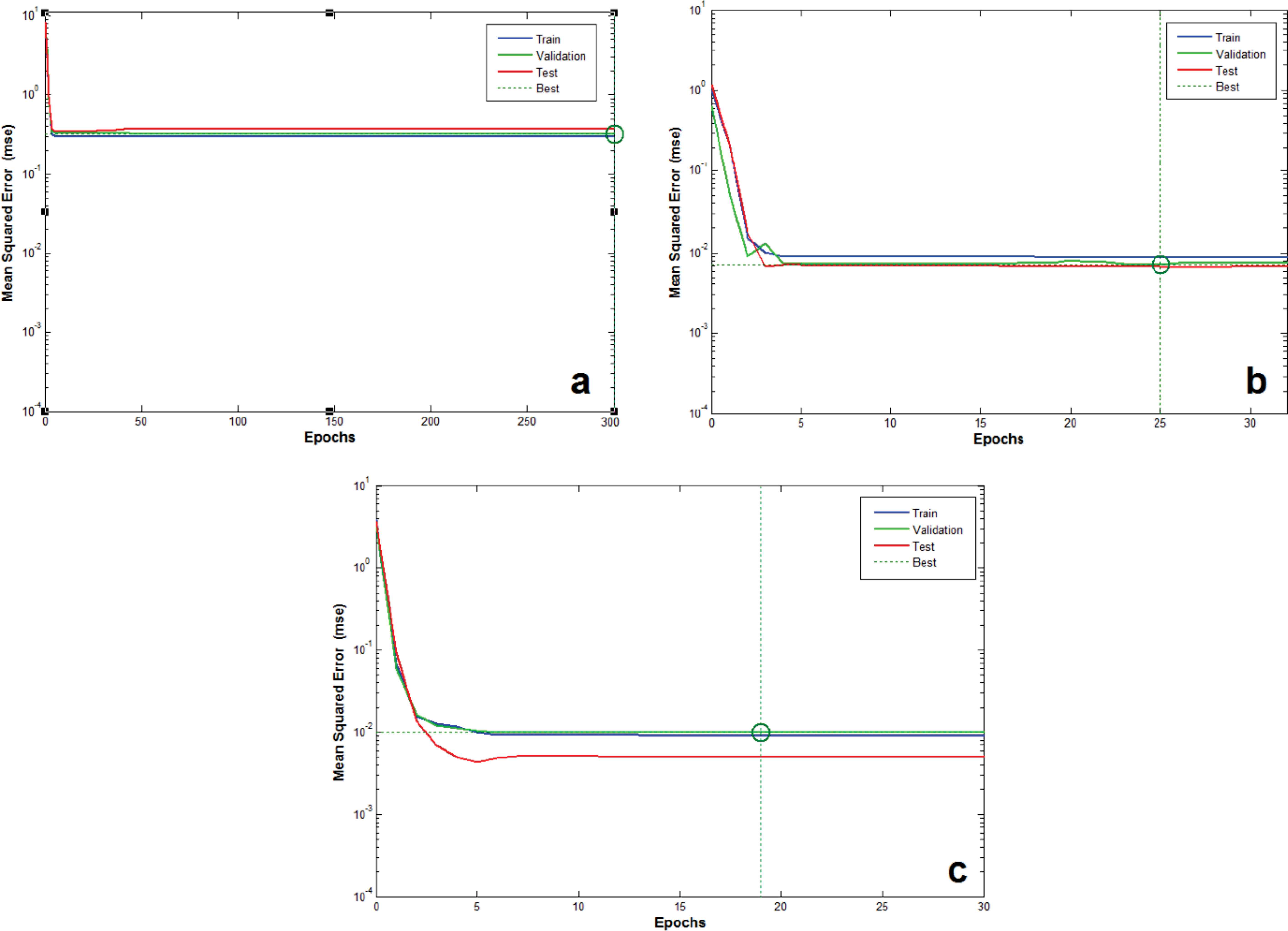
Performances of the models with regard to the MSE values versus epochs: (a) ANN model; (b) ICA-ANN model; and (c) PSO-ANN model.
The performances of the constructed models were evaluated on the basis of their R-squared values, MSE values, iterations and computation times. The corresponding index values for the ANN, ICA-ANN, and PSO-ANN models are computed and then tabulated in Table 3.
| ANN | ICA-ANN | PSO-ANN | |
|---|---|---|---|
| R-squared | 0.9216 | 0.9904 | 0.9937 |
| MSE | 0.2824 | 0.007650 | 0.005200 |
| Iterations | 298 | 25 | 19 |
| Computation Time (s) | 11.3 | 2.4 | 2.1 |
Performances of the designed models.
The R-squared values for the three techniques discussed in this work are high and close to each other. However, high R-squared values do not sufficiently result in improved models in all cases and the model may systematically over and under predict the data along the curve. To distinguish the performance differences of the different techniques, the MSE values for this case study provide better distinctions between the modelling performances.
It can be observed that the results of the ICA-ANN and PSO-ANN models are in better agreement with the plant data in comparison to that of the conventional ANN model. The improved performances of the ICA-ANN and PSO-ANN models are due to the fact that they combine the local searching ability of ANN and the global searching capabilities of ICA and PSO. In addition, as shown in Table 3, the PSO-ANN model outperformed the ICA-ANN model. The R-squared value of PSO-ANN is close to the analogous value of ICA-ANN, however, the MSE value, iterations and computation time of PSO-ANN are better than the corresponding values of ICA-ANN.
9. Conclusions
In this study, the dynamic behavior of the GDPT of a gas sweetening plant are predicted by means of hybrid models designed on the basis of the ANN modeling tool. The models can then be utilized to detect the undesirable foaming condition in the process. The models are structured using ANN, while ICA and PSO have the roles of weight initialization for the ANN models. The results of the designed models show that the agreement of the measured data with the predicted outputs of the ICA-ANN and PSO-ANN models are reasonably better than that of the ordinary ANN model. The improved performances of the ICA-ANN and PSO-ANN models against the conventional ANN model are due to the reason that they combined the local searching ability of ANN with the global searching capability of ICA and PSO. It was also established in this work that the PSO-ANN model outperformed the ICA-ANN model because PSO possesses a higher ability in global searching, requires fewer parameters for tuning, and necessitates lower computation time than ICA.
References
Cite this article
TY  - JOUR
AU  - Masoud Rohani
AU  - Hooshang Jazayeri-Rad
AU  - Reza Mosayebi Behbahani
PY  - 2017
DA  - 2017/01/01
TI  - Continuous Prediction of the Gas Dew Point Temperature for the Prevention of the Foaming Phenomenon in Acid Gas Removal Units Using Artificial Intelligence Models
JO  - International Journal of Computational Intelligence Systems
SP  - 165
EP  - 175
VL  - 10
IS  - 1
SN  - 1875-6883
UR  - https://doi.org/10.2991/ijcis.2017.10.1.12
DO  - 10.2991/ijcis.2017.10.1.12
ID  - Rohani2017
ER  -