
An Application of Dynamic Bayesian Networks to Condition Monitoring and Fault Prediction in a Sensored System: a Case Study
- DOI
- 10.2991/ijcis.2017.10.1.13How to use a DOI?
- Keywords
- Bayesian networks; anomaly detection; sensor networks; predictive maintenance; condition monitoring
- Abstract
Bayesian networks have been widely used for classification problems. These models, structure of the network and/or its parameters (probability distributions), are usually built from a data set. Sometimes we do not have information about all the possible values of the class variable, e.g. data about a reactor failure in a nuclear power station. This problem is usually focused as an anomaly detection problem. Based on this idea, we have designed a decision support system tool of general purpose.
- Copyright
- © 2017, the Authors. Published by Atlantis Press.
- Open Access
- This is an open access article under the CC BY-NC license (http://creativecommons.org/licences/by-nc/4.0/).
1. Introduction
Decision support systems (DSS) are widely used for industrial damage detection 2,6,19. It is not an easy, nor cheap, task to maintain industrial units as every component suffers damage continuously due to usage. However, there are several advantages in using automated systems to carry out this maintenance. This type of system provides a health status prediction about the monitored units 5,24, which is very useful for human beings because it gives them information about what components might be failing or are close to fail. This fact translates into an improvement in the time required to detect the failure and in the determination to detect what unit is failing.
There are a wide range of industrial environments which have different requirements. For some of them, e.g. electric companies, working without interruptions is a priority 1,15. For those cases, these decision support tools are used to carry out a preventive maintenance, helping to detect any problem and solving it as soon as possible or even before it occurs.
Different data mining techniques has been used for, what is usually called, health management 2. They use information about the machinery components to learn a behavioural model which is used to predict their health status. Usually, this kind of problems are treated as a classification one, which means that the prediction will be one choice of a finite set of options 29,30,31,32. Supervised classification techniques need data from all these different options to carry out the learning process. However, in some situations this is not the case. For instance, in a nuclear power station, there might not be data from a situation of the reactor failure. For this kind of problems there are some approaches which instead of learning a behaviour model for all the possible outcomes, they focus on the detection of anomalies with respect to standard functioning 9,25. In this work we propose a method based on Bayesian networks to detect anomalous behaviours in this type of systems, encouraged by the significant examples of successful applications of Bayesian networks to condition monitoring from 27,22, predictive maintenance from 6,3,18 and fault detection/diagnosis from 28,26.
In order to design that DSS, we will start from the methodology for detecting faults and abnormal behaviours described in 22. Afterwards, we will design a new metric to improve the behaviour of the previous methodology in some general cases. In order to demonstrate the usefulness of our new proposal, we will generate some artificial datasets and we will compare the performance between the original methodology and our proposal.
This study is structured as follows. In Section 2 we briefly introduce Bayesian networks. Section 3 contains the description of our DSS, describing as well the methodology proposed in 22. Later, in Section 4 we will explain the kind of industrial system our application will work for, and we will discuss the benefits of our proposal through an artificial dataset. Also some tests are carried out in order to evaluate its performance. Section 5 contains our concluding remarks. Finally, in Appendix 1 we describe the designed decision support web-based application, while in Appendix B we show the parameters of the Bayesian networks (probability tables) used to generate the synthetic datasets.
2. Bayesian Networks
Bayesian networks (BNs) are mathematical objects which inherently deal with uncertainty 11,13. When used for probabilistic reasoning, a BN represents the knowledge base of a probabilistic expert system. From a descriptive point of view, we can distinguish two different parts in a BN, which respectively accounts for the qualitative and quantitative parts of the model. Figure 1 shows an example of a simple BN.
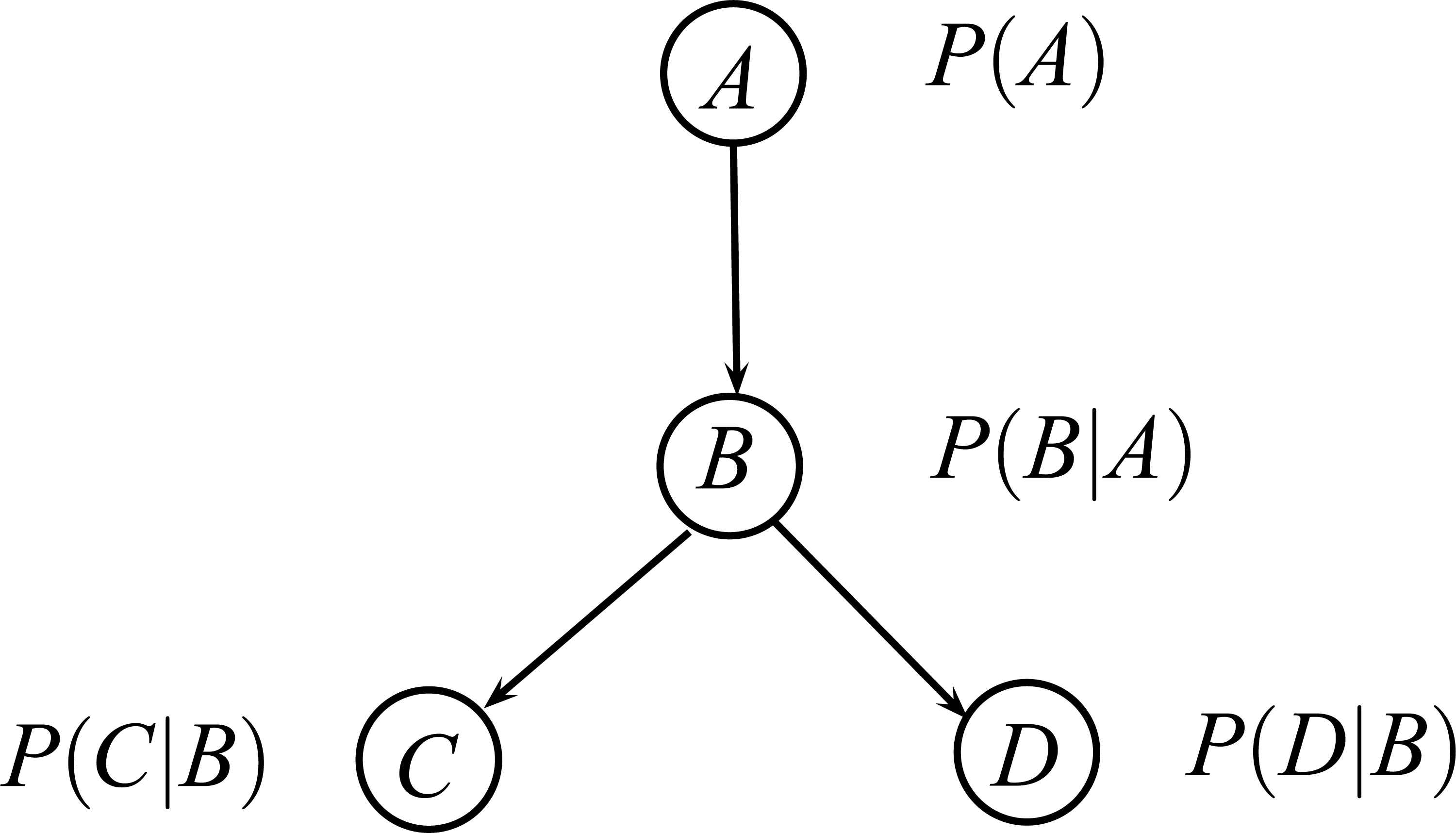
An example of BN with four variables.
The qualitative part of the network is represented by a directed acyclic graph (DAG), 𝒢, whose nodes represent the random variables in the problem domain and whose edges codify relevance relations between the variables they connect. When the network is built by hand with the help of domain experts, these relevance relations are usually of causal nature, while when the network is learnt from data, we can only talk about probabilistic dependence, but not causality. The whole graphical model codifies the (in)dependence relations among all variables and can be interpreted by using the D-separation criterion 23 in order to carry out a qualitative or relevance analysis.
On the other hand, the quantitative part of the model consists of a set of conditional probability distributions, one for each node (variable): P(Xi|pa𝒢 (Xi)), where pa𝒢 (Xi)a are the parent nodes of Xi in the DAG 𝒢. From the independences codified by the DAG, the joint probability distribution can be recovered from the BN factorization as shows the Eq. (1).
Once a BN has been built for a given problem domain, it becomes a powerful tool for probabilistic reasoning, with a great range of exact and approximate convenient algorithms to form the inference engine 4. Depending on the target domain and the availability of domain experts and/or data, the network can be manually constructed by using knowledge engineering techniques 14,12, automatically learnt from data 7,21, or combining both techniques.
An important and attractive issue of BNs is their ability to incorporate the temporal dimension, allowing in this way reasoning over time. Thus, while a static BN represents a fixed capture of the domain environment in a given instant, dynamic BNs (DBNs) allow to explicitly represent different instances of the same variables over time, as well as temporal relations between them. Figure 2 shows the most used way of dealing with DBNs in the literature 20, which consists of a basic structure (slice), which represents a static BN, together with a set of temporal relations representing the dependences from time t − 1 to time t. This structure is unfolded as many times as needed in order to forecast the values of variables at time t + k. As can be noticed, the Markovian condition is assumed in DBNs.

An example of DBN structure unfolded over time. Dashed arcs are the temporal relations.
3. Fault Diagnosis Methodology
One of the main applications of DSS is helping to carry out a predictive maintenance. It builds a model from a set of examples which is used to predict the health status of the monitored system 2. Usually, data is labelled and we know the class for each instance (if it is a normal behaviour, or on the contrary if some component is failing), so supervised data mining techniques can be used to build the prediction model. However, sometimes this information cannot be acquired, and other approaches have to be used. For example, nearest neighbour based anomaly detection techniques uses the definition of a distance or similarity measure between data instances to determine if an example is an anomaly or not 47,46. Clustering based anomaly detection techniques tries to group similar data instances into clusters. Afterwards, if an incoming instance does not belong to any cluster it would be an outlier 33,34. Sometimes, this assumption is relaxed and an incoming instance is marked as an outlier if it is far away from the centroid of the cluster that it belongs to 35,36, or if it belongs to a sparse cluster 37,38. Statistical anomaly detection techniques say that an observation which is not generated by the assumed stochastic model is an anomaly. These models are built from data using parametric 45,44,43 or non-parametric techniques 42,41. Also, classification based anomaly detection techniques has been widely used 40,39,22. These techniques learn a model which distinguishes between normal and anomalous classes.
In this paper we aim to propose a failure detection tool whose goal is to detect generic failures from the information collected in a sensored system. This tool is based on a technique included in the last mentioned group (classification based anomaly detection techniques), and in more detail, using Bayesian networks as models to represent the behaviour of the system. Therefore, our BN-based system is not targeted for the detection of a concrete type of failure in a particular machine or set of machines, but on the contrary, what we aim is to be able of detecting any anomalous behaviour of the system (that can be inferred from sensors readings). Obviously, dealing with such a so general problem represents a disadvantage with respect to tailored systems, due to the absence of problem domain knowledge. On the other hand, it is more general and realistic because we can detect previously unknown failures. In our case, the system being monitored can be viewed as a black box (Figure 3).
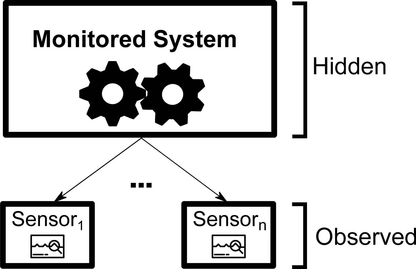
General system structure
We cannot consider to deal with this problem by using supervised classification methodologies because of the nature of the input data. In particular, we do not have data about each possible wrong behaviour of the system, in fact, we only dispose of data corresponding to one or more status of the machinery working in absence of failures. Our goal is to predict whether the current behavioural state of the physical system is correct or on the contrary it stands for some kind of failure. Therefore, instead of a fully supervised classification methodology, we opt for the use of an anomaly detection 2 based one.
In this type of methodologies, a model is constructed to represent the failure-free behaviour of the physical system, and it is used to check if an incoming sensor reading does not match it, producing a failure warning (or alarm) in such a case. We will start from the methodology detailed in 22, adapted to our case of such general problems. However, as we will discuss in Section 4, the previous methodology has problems in some specific circumstances. In order to improve the performance of our DSS in such cases, we have introduced a new model definition (in addition to the failure-free behaviour one) to represent the anomalous behaviour. As an overview, the workflow of our DSS is shown in Figure 4.
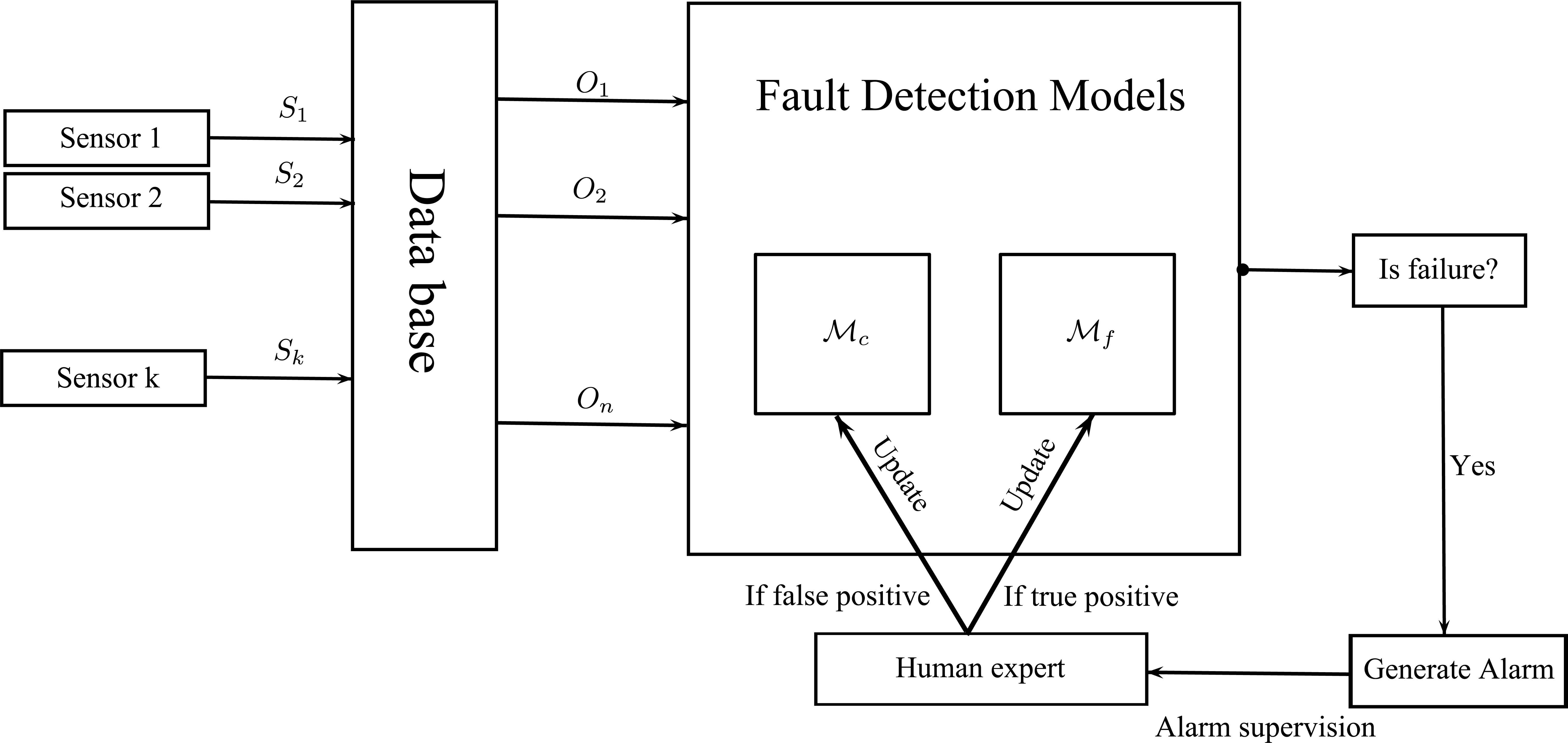
System behaviour
Every cycle (reading-detection) has the following behaviour: (1) readings are taken from the sensors and stored in a data base; (2) these readings, possibly manipulated, give rise to the observations entered into the expert system for classification; (3) the probabilistic expert system (composed of two Bayesian networks) computes the prediction (fault or non-fault); (4) if a possible failure has been identified, an alarm is generated and a human operator supervises it; finally (5) the knowledge-base is updated according to this information (false or true positive alarm).
Therefore, the proposed DSS has been designed as a generic tool, where no specific problem domain has been considered. Nevertheless, it is noteworthy that if some previous knowledge is available, it can be incorporated to our system, as this is one of the main advantages of using a Bayesian network to represent the knowledge base. In order to deal with a so generic failure detection system, we impose the two following assumptions:
- •
The tool needs a first stage in which it collects data from the monitored system (sensors readings) working properly, i.e. without failures. From these readings, the system will construct/learn a correct behaviour model. This is not a hard assumption, since long periods in the absence of failures are common in industrial machinery.
- •
Some degree of supervision is needed. As we do not have prior information about how a failure looks like, once a suspicious behaviour is detected from the sensors readings because it deviates from the (learnt) correct behaviour model, we need that a human operator confirms if the detected anomalous behaviour actually corresponds to a failure in the system or if it is just a false positive. This information will be used as feedback to improve the prediction models.
This section is structured in the following subsections. First, in Subsection 3.1 we are going to describe both models for failure-free and anomalous behaviour. Then, in Subsection 3.2 we detail the metrics used in our DSS and how we combine them to detect anomalous behaviours. Finally, in Subsection 3.3 we detail how these models are updated when a human operator tells the system about false or true positive alarms.
3.1. Bayesian networks to detect anomalous behaviours
As we said before, we are going to use two Bayesian networks: ℳc, the model to represent failure-free behaviours and ℳf for anomalous behaviour.
Bayesian networks assume discrete values as inputs. However, this is not usual in the case of sensor readings, e.g. temperature. One option would be to use Hybrid Bayesian networks 48 instead, which can deal with real input values using a conditional gaussian model. However, this approach has some drawbacks, as imposing certain restrictions about the topology of the network. Another option, used in this work, consists on applying a pre-processing discretization step, where the discretization intervals can be provided by domain experts, obtained by applying some unsupervised discretization technique 16 or just using equal width binning.
In the following subsubsections we detail how ℳc and ℳf are built (Subsubsection 3.1.1 and 3.1.2 respectively).
3.1.1. Probabilistic model for failure-free behaviour: ℳc
The physical system for which we intend to carry out the predictive maintenance can be in a serie of (hidden) states. We have no direct access to these inner states, but to some observable measures provided by a set of sensors (e.g. light, vibration, temperature, etc.) attached to the machinery. Let us assume we have n sensors {S1,…,Sn} each one taking values in
The main goal is to obtain a probabilistic model which represents the behaviour of the system working properly, that is, without any defective component and so assuming correct sensors readings. This probabilistic model, which we will call ℳc needs to deal with the n sensors but also with the temporal relations among them, as the evolution on the value of a given sensor, will provide clues on its correct or incorrect functioning. Because of these requirements, we have chosen the formalism of DBNs 20 to represent our knowledge base.
For the sake of simplicity and because of the lack of prior domain knowledge we have resorted to a simple DBN model with fixed graphical structure. In the model, each sensor is independent of the restb but depends on itself at time t −1, that is, there is no arcs of type Si → Sj, but we include temporal arcs of type
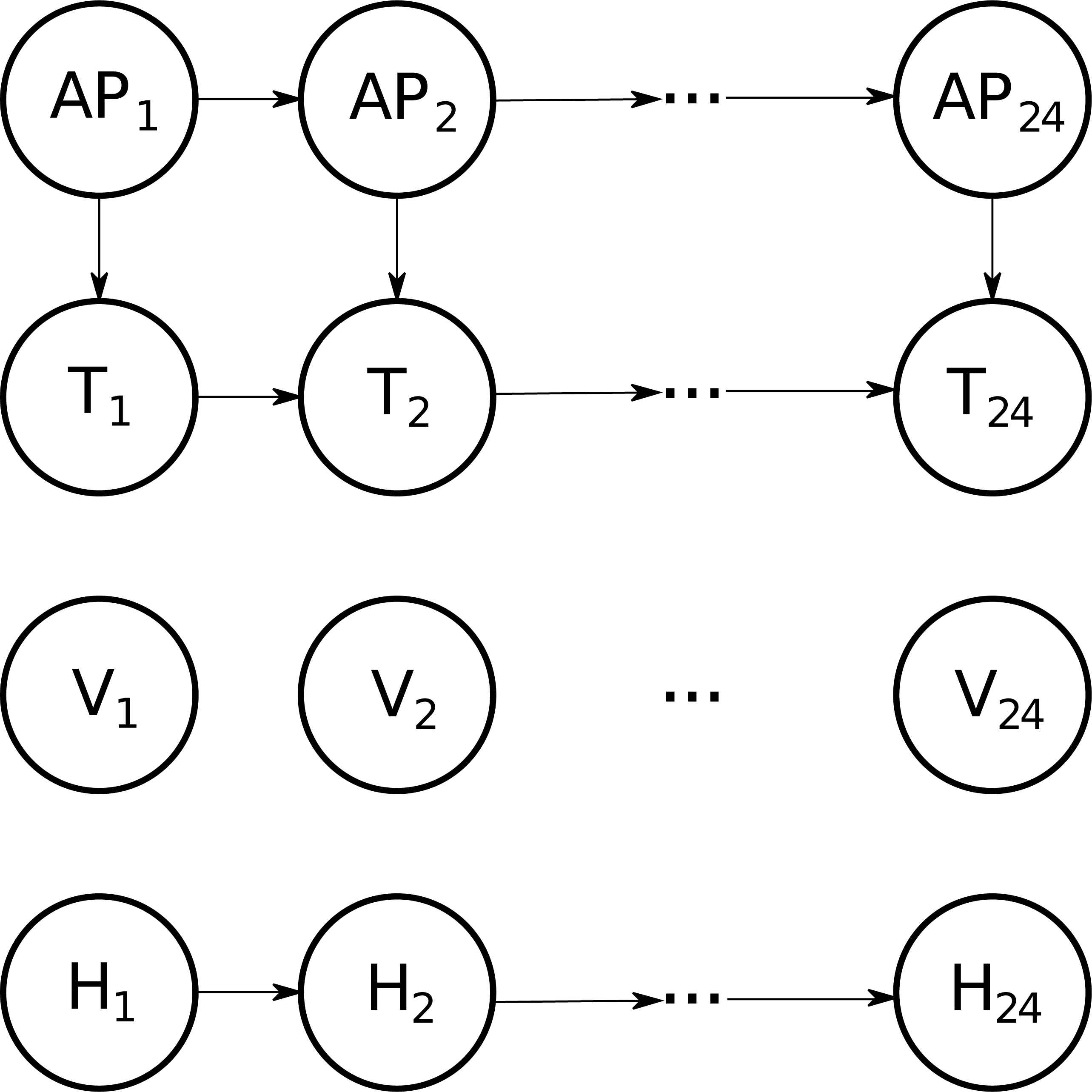
In practice, for better readability reasons, we actually deal with a static BN, in which temporal relations are taking into account by unfolding the DBN for a given number of temporal slices (in this work equals to 24). In fact, the way to procede with DBN is to unfold 1 layer at each time, forgetting (or not) the past layers. However, we determined to use this strategy (unfolding the 24 layers at once) because of the monotonous behaviour of these types of environments: even if the machinery carries out different operations depending on the hour of the day, this pattern is usually the same every day (24 hours). The resulting model is shown in Figure 5, where we represent 24 consecutive hourly measures for each sensor, that is, we model a full day of the physical system.

Graphical structure of the unfolded DBN
Once we have described the structure of our probabilistic graphical model ℳc, we need to provide the numerical parameters, that is, the conditional probability tables. To do this we use the dataset containing sensors readings captured during a period of correct functioning of the monitored system. Our first task is to transform the captured dataset, containing hourly readings for the n variables (sensors) to a new one containing 24 × n variables. The process is described in Figure 6.
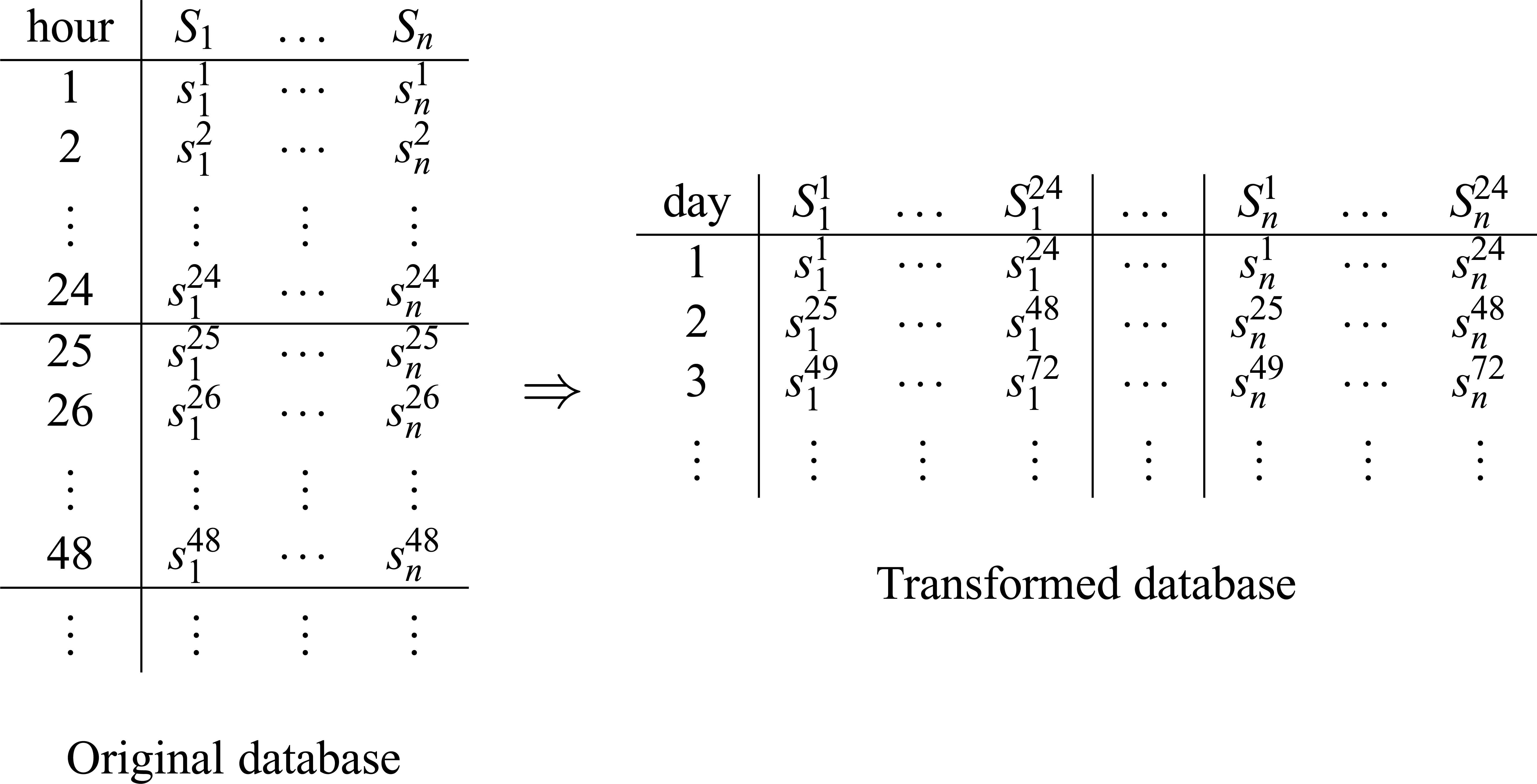
Database transformation
From the transformed dataset, where each
3.1.2. Probabilistic model for anomalous behaviour: ℳf
Apart from ℳc that models the normal behaviour of the physical system, we propose the use of a failure model ℳf which models the anomalous behaviour of the physical system, that is, how the readings look-like when some failure is happening or is close to happen. In our case, as we have previously described, due to the generality of the approach we have no data to learn this model. Nonetheless, we have decided to use a random failure model, ℳf, which has the same graphical structure as ℳc, but whose parameters (local probability distributions) have been randomly generated using an uniform distribution. The rationale behind using this model is that normal sensors readings will have a high likelihood of being generated by ℳc and a very low likelihood of being generated by ℳf. However, in the case of abnormal sensors readings, the likelihood with respect to ℳc should decrease, while the one with respect to ℳf shoud increase or at least do not change substantially.
3.2. Anomaly detection procedure
After learning ℳc and generating ℳf, they are used to process new sensor readings. The goal is to predict whether a new reading represents a failure-free behaviour for the machinery, or on the contrary it represents some anomalous behaviour, which can be associated with a failure or with a warning that indicates a forthcoming failure.
In the following subsubsections we present two metrics and the way they are combined in order to classify input readings into failure-free and anomalous behaviours. In Subsubsection 3.2.1 we show a metric based exclusively in ℳc, used in the methodology proposed in 22. Then, in Subsubsection 3.2.2, we explain our proposal to improve the performance of the previous methodology. Finally, in Subsubsection 3.2.3 we detail how we detect anomalous behaviours combining the previous metrics.
3.2.1. Metric conf (e)
The methodology proposed in 22 is based on measuring the conflict between the model and the sensor readings. A fault (an anomaly) will be detected when that measurement reaches a threshold. To detect if a particular case or reading is coherent with the model ℳc or not, it uses a procedure which is based on the well known conflict (conf) measure proposed in 10 (see also 11). The measurement is described in Eq. (2).
The idea behind conf measure is that findings coherent with the model should be positively correlated, thus, Pℳ (e) should be greater than the product of independent (marginal) probabilities, Pℳ (e1),…,Pℳ (en). Therefore, a negative number would indicate that e is coherent with the model ℳ, while a positive one is an indicator of a conflict. The bigger the number, the more probable the conflict is.
From a computational point of view, computing conf (e) requires two propagations (inferences)11 over the probabilistic graphical model: (1) in the first one, no evidence is entered into the network, so, marginal probabilities P(e1),…,P(en) are obtained; and (2) in the second one, all the findings e1,…,en are entered as evidence, and P(e) = P(e1,…,en) is obtained after the propagation by computing in any node the normalization constant.
In our case, as we are interested in the predictive maintenance of the machinery, we use as findings the sequence of readings from time ti to time tj, where 1 ≤ i, j ≤ 24 and w = j − i is a positive integer. This is because a failure usually does not happen abruptly, but gradually, so we consider the sequence of readings in order to evaluate possible trends. However, we consider a maximum time window size w (temporary difference between tj and ti), because if we take into account the whole set of readings, the information provided by the last measurements would have a small impact as they are diluted by the rest of the readings.
3.2.2. Metric rcf (e)
The previous metric detects anomalies paying attention to the dependencies between variables. As it will be discussed in Section 4, an uncommon sequence of readings might be considered a failure-free behaviour. In order to improve the performance of our DSS, we will introduce a second measurement (which uses both models, ℳc and ℳf). This new measure, called ratio correct vs fault (rcf), is shown in Eq. (3).
At the begining, when the parameters of ℳf has been initialized randomly, a change in the behaviour of the system should not affect substantially to Pℳf (e). On the contrary, if that situation corresponds to an abnormal behaviour, Pℳc(e) should decrease and therefore the ratio rfc(e) should increase. On the other hand, if readings correspond to a normal situation, Pℳc(e) should be higher than Pℳf (e) as the parameters of ℳc has been learnt from data in abscence of failures. Moreover, when the model ℳf has been updated with data from anomalous behaviours, the measure rcf (e) should improve its performance as the parameters of the model ℳf has been updated using data of anomalous situations, and therefore Pℳc(e) and Pℳf (e) should behave oppositely.
As in conf(e), we will use as evidence the sequence of readings from time ti to tj, where e has the same meaning as in Eq. (2) and the same window size w is used.
3.2.3. Use of conf (e) and rcf (e) for anomaly detection
In this section we are going to explain how we use conf(e) and rcf(e) to detect anomalous behaviours. The basic idea behind this is to use two thresholds, one for each metric. Each time one measure is greater than its associated threshold, then an anomalous behaviour will be detected. However, we realised that using the whole evidence e to compute each measure has some drawbacks. As aforementioned, it is an unusual situation that a component fails, and usually when it happens only a few sensors would be involved. Because of that, if the system is composed of a large number of sensors, the information of an anomaly can be diluted by the rest of sensors and the failure detection can be noteless.
In order to deal with that problem, the previously described measures (conf and rcf) are separately computed for each different sensor in our system, using as evidence the readings from that sensor and from all its ascendants in the network (for time window w). This gives us information about the probability that a concrete sensor reading comes from an anomalous behaviour or not. Moreover, we are able to detect if there is a failure on the machinery and if so, the defective component.
Finally, we use the information of all these individual measures to decide if the input represents a (forthcoming) failure, and so an alarm must be fired. We have set two thresholds (tconf and trcf), one for each measure respectively. If any of the computed measures is greater than its associated threshold, then an alarm (related to the evaluated sensor) is triggered. For the sake of clarity, in our experiments (see Section 4) we do not pay attention to what component is failing, but only if any component in the whole system is failing or not.
3.3. Models updating
Even if no domain knowledge is used to build the model, the information about its performance can be used as feedback. Therefore, if at some point the system triggers an alarm, a person who checks the status of the monitored system can tell the DSS if the behaviour has been correctly classified or not. This information can be used to update the models and improve their predictions.
Given a certain alarm, if it is marked as a false positive it means that data come from a correct behaviour, so the model ℳc will be updated using this information (as described afterwards). On the contrary, if it is marked as an actual failure, it means that data come from an anomalous behaviour, so the model ℳf will be updated. The data used to make the model updates correspond to those contiguous readings from the first detection of the alarm to the last one (the reading before data is considered again as normal behaviour).
The update process keeps the model structure invariable but changes the parameters (probability tables). Let
The parameter α determines the “memory” of the system about past readings. Its range is [0 − 1]. As it closes to 0, it gives more importance to the information about the past. Therefore, the model requires more time to be adapted to a new behaviour. On the contrary, as it closes to 1, the model tends to represent exclusively the recent behaviour of the monitored system, forgeting the past behaviour in a small window of time.
4. Simulated Case of Study
In this section we are going to test the predictive capability of the original methodology explained in 22 and compare it with our proposed DSS. In order to do that, we are going to generate synthetic data representing different scenarios. Our aim is to test the following situations. The system has been trained using data in abscence of failures. Then:
- •
The behaviour does not change, so no alarms should be triggered.
- •
The behaviour suddenly changes. Alarms should be triggered, but two scenarios can be tested in this case depending on the given feedback: It comes from an anomaly, or from a change in the behaviour of the monitored system.
For that, we have designed a simulated environment with four different sensors usually presented in industrial machinery: Temperature (T), Humidity (H), Vibration (V) and Active Power (AP). To generate the synthetic data from that environment, we have modeled its behaviour using a Bayesian network ℬb and then we have generated samples from it. In order to represent a change in the behaviour of the monitored system, we have used two alternatives:
- •
Keep the Bayesian network structure of ℬb but change its parameters.
- •
Change the structure of the Bayesian network ℬb.
Next we are going to explain in detail the models and the process to generate the synthetic data from them.
The first model ℬb, used to generate the initial behaviour and the first alternative, is shown in Figure 7. We have set a direct dependence between Active Power and Temperature, and also between Humidity and Vibration. These dependences have been replicated in the 24 hourly layers, that is from [0:00-1:00) to [23:00-0:00). Regarding the domain for each variable, we have considered that the four variables take values in the set {Low, Medium, High}. Therefore, as we deal directly with discrete values instead of real numbers, there is no need to apply the discretization stage.

Graphical structure (ℬb) for the simulated case of study
After setting the structure of the model, we have parameterized it into two different ways:
- •
Basic behaviour, which represents the usual machinery functioning (𝒲b). In this case, ℬb has been parameterized in the following way: all sensors tend to generate the Low value with more probability than the Medium one, and this Medium with more probability than the High one. Furthermore, and due to the dependences in the graphical model, Vibration and Temperature tend to follow the measures of Humidity and Active Power respectively, and each sensor tends to follow its own measure in the previous layer (time). To see the specific values, see Table B.1 in the Appendix B.
- •
Alternative behaviour 1, which represents a situation in which we detect more vibration than usually (𝒲a1). In this case, the network ℬb is parameterized in a different way: Temperature, Humidity and Active Power have a similar behaviour as in basic behaviour (𝒲b), but Vibration will tend to get higher values. Specific values for Vibration variables are shown in the Appendix B, Table B.2.
The second model structure, ℬa is similar to ℬb but any dependence of the variable Vibration has been removed (see Figure 8). The parametrization of this network is as follows:
- •
Alternative behaviour 2, which represents a situation in which vibration readings follow the uniform distribution (𝒲a2). Therefore, we take (ℬa) as basic structure and parameterized it according to the following description: All the states of Vibration have the same probability while the remaining probability distributions are set as in the basic behaviour (𝒲b).
Alternative graphical structure (ℬa) for the simulated case of study
In order to obtain the datasets for the simulations, the models are sampled by layers (first t = 1, then t = 2, etc.) and inside each layer, a probabilistic logic sampling 8 is guided by a topological ordering (e.g. AP, H, T, V). We consider two cases:
- •
Initial time slice (t = 1). First, variables without parents in the network are (independently) sampled from their marginal distribution. That is, P(AP1) and P(H1) for 𝒲b and 𝒲a1, and P(AP1), P(H1) and P(V1) for 𝒲a2. Once the values for these variables are known (call them ap, h and v), the rest are sampled from the marginal distributions: P(T1|AP1 = ap) and P(V1|H1 = h) for 𝒲b and 𝒲a1, and P(T1|AP1 = ap) for 𝒲a2.
- •
Rest of time slices (t ≥ 2). Now the values for all the variables in the time slice t −1 are known, therefore the marginal distribution to be sampled by order are: (1) P(APt|APt−1 = apt−1), P(Ht|Ht−1 = ht−1), P(Tt|APt = ap,Tt−1 = tt−1) and P(Vt|Ht = h,Vt−1 = vt−1) for 𝒲b and 𝒲a1; (2) P(Vt), P(APt|APt−1 = apt−1), P(Ht|Ht−1 = ht−1) and P(Tt|APt = ap,Tt−1 = tt−1) for 𝒲a2.
From these models we have sampled four datasets. Each one contains 4320 readings (〈ap,t,v,h〉), corresponding to 6 months, 30 days per month and one reading every hour.
- •
BasicT. This dataset is sampled from the Basic behaviour model 𝒲b and will be used to Train the correct behaviour model (ℳc).
- •
BasicV. This dataset is sampled from the Basic behaviour model 𝒲b and will be used to validate the correct behaviour model (ℳc).
- •
AlternativeU. This dataset is sampled from the Alternative behaviour model 1 𝒲a1 and will be used in two different ways, to update the correct and failure behaviour models (ℳc and ℳf). In other words, telling the DSS that alarms correspond to a change in the behaviour of the system or to an anomaly.
- •
AlternativeR. This dataset is sampled from the Alternative behaviour model 2 𝒲a2 and will be used as well in two different ways, to update the correct (change in the behavuour of the system) and failure (anomaly) behaviour models (ℳc and ℳf).
4.1. Simulation data
In this section we will discuse how the two models ℳc and ℳf and their behaviours evolve during the simulation. The parameters used are w = 24 for the time window, tconf = trcf = 1.0 for the alarm thresholds and α = 0.5 for updating the models. Note that even if w = 24, in this experimentation the nodes in the last layer of the Bayesian networks are not connected to the nodes in the first layer. That means that when t = 1 it only uses data from the first hour of the day, while when t = 24 it uses the information of the whole day (it can be seen as a variable window size, from w = 1 to w = 24). The experiment is as follows.
Firstly, we create the structure of both models ℳc and ℳf as described in Section 3, that is, dependence relations between sensors in the same layer are not included, because we suppose that we do not have such domain information. Of course, if these relations (or others) are available as problem domain knowledge, they can be added to the graphical structure. Then, we use BasicT dataset to learn the parameters for ℳc, that is, P(AP1),P(T1),P(H1),P(V1) and P(APt|APt−1),P(Tt|Tt−1), P(Ht|Ht−1), P(Vt|Vt−1). In the case of ℳf these distributions are initialized at random (uniform distribution).
After ℳc and ℳf have been built, five different situations are tested: BasicV is used to validate the correct behaviour model (ℳc); AlternativeU is interpreted first as normal behaviour and afterwards as anomalous behaviour, in order to check the adaptability of the system; Finally, the same experimentation is done with the data set AlternativeR.
For all the experiments we show three graphics. The first two correspond to the measures (per hour) for conf and rcf respectively, while the last one is the number of detected anomalies per day by our proposal, and so the number of alarms sent. For the first and second graphics we show the first 1440 (two months) measures instead all the 4320 (the whole six months) because graphics get clear and the change in the data trend is inappreciable thenceforth.
4.1.1. BasicV as correct behaviour
The dataset BasicV is used to test the proposal. As BasicV comes from the same distribution as BasicT, the process should detect few anomalies, and so the number of alarms sent should also be small. In this case, as we know the inputs (sensors readings) correspond to correct machinery functioning, the operator will identify the alarm as false and model ℳc will be accordingly updated/refined.
As we can observe in Figure 9, the proposed process works properly and the number of alarms stays low or even decreases as the days go on and the model is refined. In this case, both measures, conf and rcf, give the maximum value in the early hours of the day and the minimum at the last one. This is because at the beginning of the day is when these measures takes the lowest amount of information, as we only use readings from the same day. Because of that, as the day progresses and more information can be used, both conf and rcf go to their lowest values. As both measures have a similar behaviour, the performance of the initial methodology and our proposal would be very similar.

Testing process over BasicV. Same operation mode.
4.1.2. AlternativeU as correct behaviour
The dataset AlternativeU is now used to test the proposal, but interpreting it as a change in the operation mode of the machinery. That is, something in the functioning, environmental condition, etc. has changed, which produces the differences in the sensors readings regarding the data used for training, however, each time an alarm is sent, the operator marks it as correct behaviour (i.e. a false positive).
As we can observe in Figure 10, the number of anomalies detected is very low even at the first days. This is because the model ℳc is quickly updated/refined according to the false anomalies detected, and the new data is understood as normal behaviour. It is worthpointing that only vibration readings has changed with respect to the basic behaviour (BasicV), and this change consists on higher values for these readings over the time. Therefore, the most relevant change in the probability distributions will lies in P(V1), because in the following layers (as well as for the basic behaviour BasicV) sensors tend to follow their own measures in the previous layer.

Testing process over AlternatuveU interpreted as no failures.
Finally, again as both measures have a similar behaviour, the performance of the DSS would be very similar, whether we use the proposed improvement or not.
4.1.3. AlternativeU as anomalous behaviour
Now we use the same dataset AlternativeU but understanding its readings as failures. Thus, we start with the model ℳc trained with BasicT data. As in this case all the alarms sent by the algorithms are confirmed as anomalies by the operator, the updated model is ℳf and not ℳc.
As we can observe in Figure 11, in the first days the number of anomalies detected is small. However, after a few days, when ℳf is refined, almost all the (24) readings are classified as anomalies. We can see that the values of conf are similar to those in the previous case, where AlternativeU is understood as normal behaviour (just in the early hours of the day values tend to be higher). This is due to conf detects anomalies paying attention to the dependencies between variables, and as we said above, the model ℳc learnt that sensors tend to follow their own measure in the previous layer, so if vibration readings are high it will consider the most probable next reading will be also a high value. On the contrary, once ℳf is refined, rcf gets higher values as Pℳf (e) ≥ Pℳc(e).
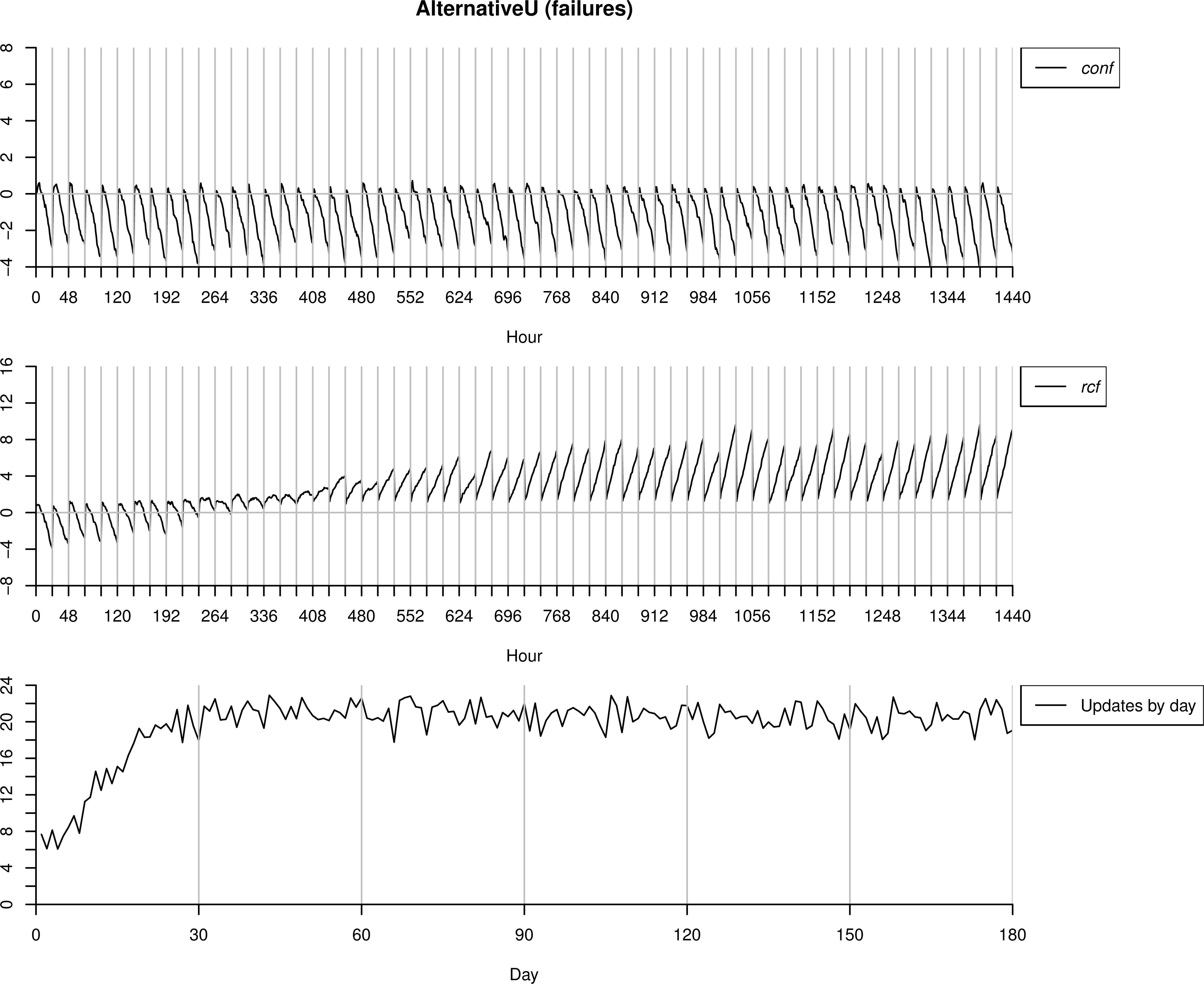
Testing process over AlternatuveU interpreted as failures.
In this case, the measure conf does not detect any anomalous behaviour. However, once the first triggered alarms are marked as failures, rcf starts to identify correctly the new ones, and is directly responsible of the increase in the number of alarms sent. In this case, our proposal is able to adapt the new situation and classify the new instances as anomalous behaviour while the methodology which only uses the measure conf is not.
4.1.4. AlternativeR as correct behaviour
The dataset AlternativeR is now used to test the proposal, but interpreting it as a change in the operation mode of the machinery. That is, something in the functioning, environmental condition, etc. has changed, which produces the differences in the sensors readings regarding the data used for training, however, each time an alarm is sent, the operator mark is as correct behaviour.
As we can observe in Figure 12 the number of anomalies detected is high at the first days, while this number decreases as the model ℳc is updated, and the new data is understood as normal behaviour. This is because now we are in a more complex situation than when using AlternativeU as correct behaviour. Now, apart from updating P(V1), also P(Vt|Vt−1) needs to be re-trained in order to incorporate the behavioural change in ℳc.
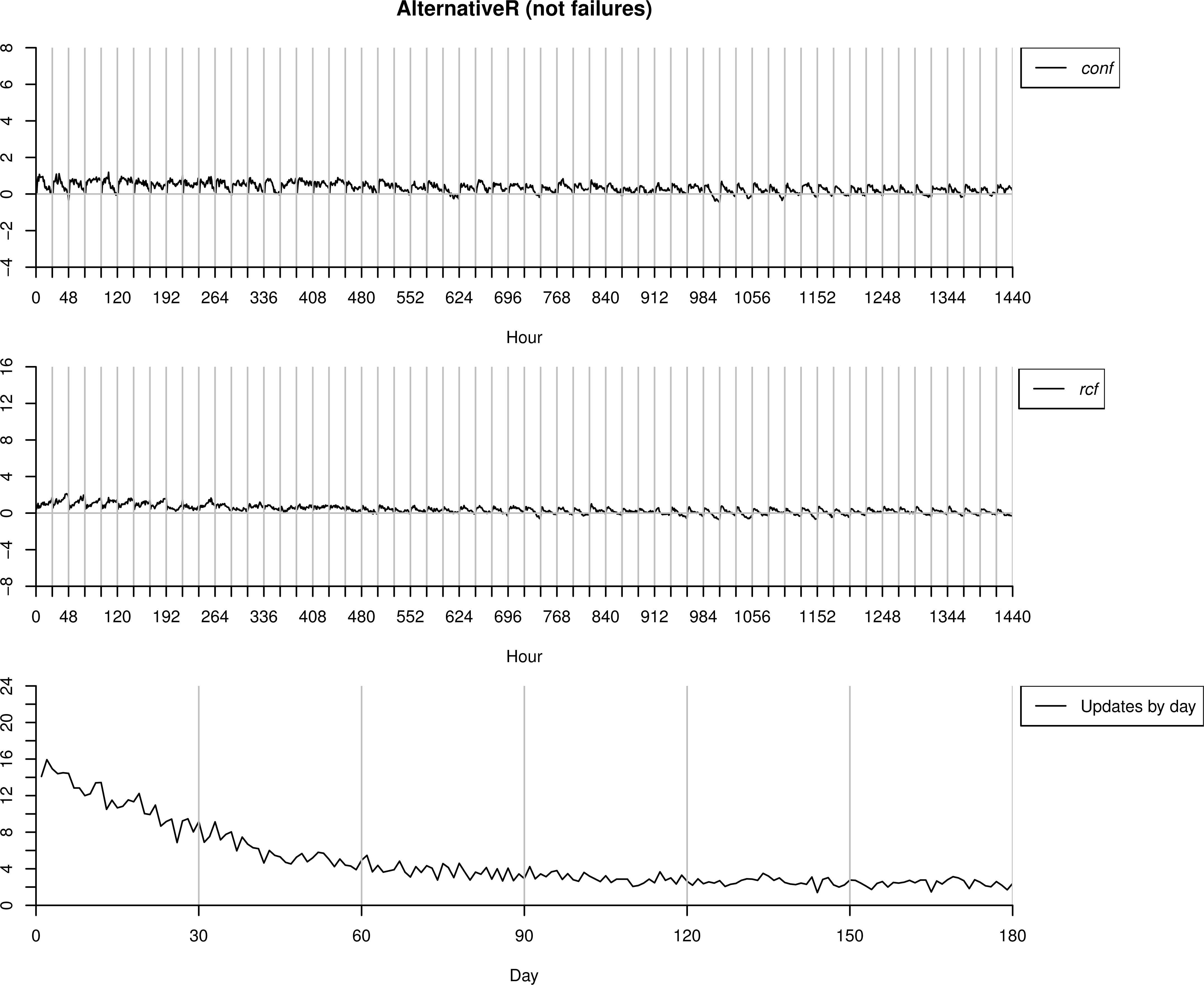
Testing process over AlternatuveU interpreted as no failures.
4.1.5. AlternativeR as anomalous behaviour
Finally we use the same dataset AlternativeR but understanding it as failures. Thus, we start with the model ℳc trained with BasicT data. As in this case all the alarms sent by the algorithms are confirmed as anomalies by the operator, the updated model is ℳf and not ℳc.
As we can observe in Figure 13, in the first days almost all the (24) readings are classified as anomalies. It is worthpointing that, even if it looks like both measures conf and rcf have the same importance in this case, the first measure has more importance. If we pay attention to the first day, we can see that rcf follow the tend of conf. What is really happening is that first conf detects the anomaly (but not rcf), and after a few updates of ℳf then rcf will be able to detect as well as conf the anomalies (but no before these first updates). However, our proposal uses a combination of both measures. Therefore all the cases are detected correctly as failures, so the performance of both methodologies would be quite similar.
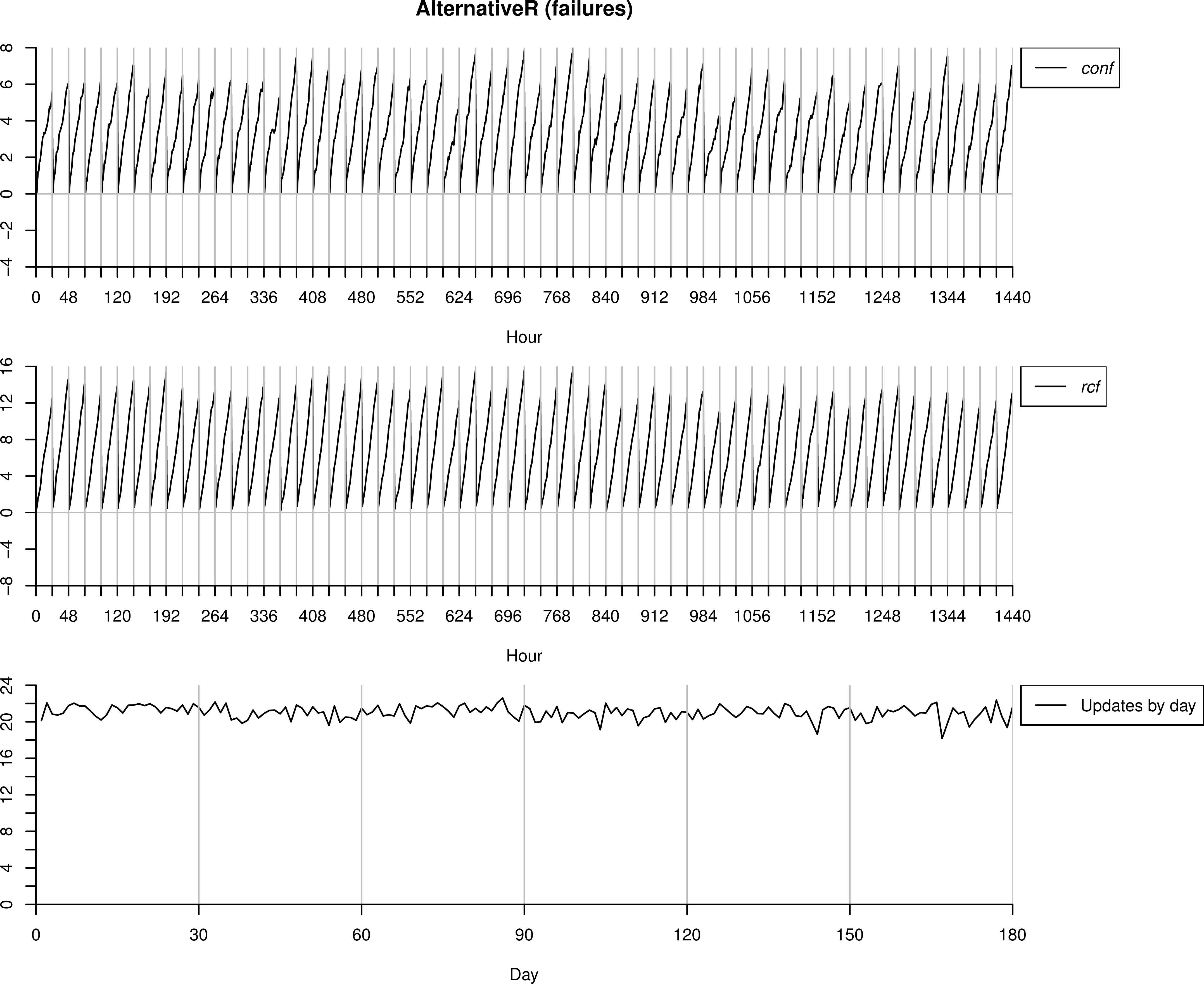
Testing process over AlternativeU interpreted as failures.
5. Conclusions
We have designed a general and robust decision support system tool for health management in industrial environments. The core of the system is a probabilistic expert system based on dynamic Bayesian networks. Fault detection is based on both conflict analysis and likelihood-ratio test.
Different types of failures has been tested, and due to the use of two measures to trigger alarms, they have been correctly detected. It is worth pointing that the second measure based on likelihood-ratio test only affects directly in one of the tested cases. However, it is an important case because it could represent a change in the usual operation mode of the monitored system. Additionally, although dependences between sensors are not considered by default, if some knowledge about the problem is available it can be included as a consequence of using Bayesian networks for modelling.
The expert system-based application has been implemented using multi-platform technology, so it can be deployed on any operative system. In order to avoid problems derived from editing the system configuration in parallel, we only allow one person to be editing the the system description at the same time. Because of that, it is recommendable that only one person would be the manager of the system.
Finally, even if the tool can be used on any kind of system, the time window w and the thresholds used to trigger alarms have to be fixed by an expert in order to obtain a good performance.
Acknowledgments
This work has been partially funded by FEDER funds, the Spanish Government and JCCM through projects TIN2013-46638-C3-3-P, TSI-020100-2011-140 and PEII-2014-049-P. Javier Cózar is also funded by the MICINN grant FPU12/05102.
Appendix A Application
The designed software is used as a DSS, so it can be used for both monitoring data and check if the system might be failing or not through the predictions. It follows the web-like client/server model: the information is managed and stored in a centralized system (the server) and clients can access to this information on demand.
On the server side we have two components, which can be deployed in the same machine or not. These are the database server and the web page server. The first one stores the data provided by the sensors, while the web page server provides a web interface for clients to use the application. The technology used to construct the models and make predictions is JAVA, and PHP to generate the web page and to implement web services (used by clients throughout AJAX). There are also some XML files to store information about the monitored system and preferences that clients can configure.
On the client side we use HTML5 plus Javascript to generate the webpage. It also will use AJAX to dynamically load the requested data.
The monitored system is logically divided into a hierarchical structure (see Figure A.1). Motes are the basic components which represent the physical sensors defined by the way we can access to their measures. To give a flexible abstraction layer, the way we can access to those measures is through a database. Hence, physical sensors send their measures to a server in charge of storing the data in a database. Because of that, there is a small delay introduced between the sensor readings and its processing in our DSS. However, for the scope of this application, this delay is assumable.
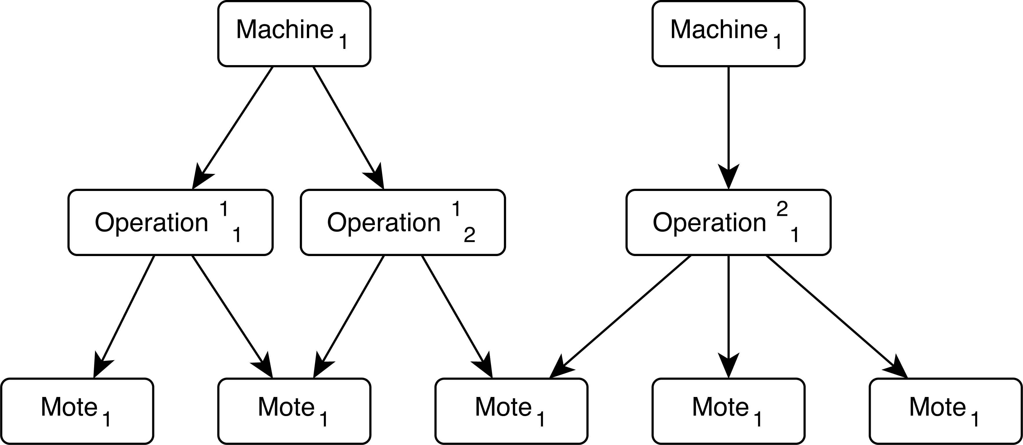
Logical hierarchical structure of the monitored system.
Machines represent a whole working unit, formed by a set of motes. It is not required that the sets of motes are disjoint. This allows the user to specify physical working units (physical machines with their associated sensors) as well as logical working units (a set of components in charge of some specific tasks, which might be shared between different physical machines).
Operations are associated with machines. They are represented by a subet of sensors (motes) from the associated machine. This is useful because sometimes is not desirable to monitor all the sensors of a particular machine, i.e: if we know the activity of a machine under supervision (cutting, polishing, etc.) we probably would prefer to monitor only the sensors allocated in the module in charge of doing that operation.
In Figure A.2 we can see the interface to manage the motes configuration. Throughout this interface we can specify the whole set of sensors used in our environment.

Example of use: Motes management.
Respect to the visualization, the interface is divided into two parts. The first one, designed to manage machine and operation definitions, as well as to monitor the sensor readings. The second part of this interface corresponds to the health status prediction.
We can see the first part in Figure A.3. For the management, we can select the desired machine or operation from their respective drop list and use the edit or remove buttons. To add new machines or operations, the proper option appear in the drop lists.

Example of use: monitoring data.
For the monitorization, the requested data is plotted in two different widgets: a speedometer and a timeline. The first one is used to show the last measure while the last is used to see the trend. In time-line widgets we can define intervals and associate colors to each one. Finally, we can set a time window to select the data to be monitored. Every fixed amount of time (specified in a configuration XML file) this window time will go forward the same period of time.
The second part of this interface corresponds to the health status prediction (see Figure A.4). We can learn the models specifying a period of time (data in that interval will be used to build such models), or delete them in order to re-learn later. Once the model has been learnt we can see the measures given by the functions conf (e) and rcf (e) described in section 3 throughout two timeline plots. When the interpretation of these formulas means a failure alert, this information is shown in the table below.

Example of use: health status prediction.
Appendix B Bayesian network parameters
In this appendix we are going to detail the parameters for the BN ℬb. Note that the parameters for the BN ℬa are the same but those for the variable Vibration, which are 0.33 for each one of its three possible values (Low, Medium and High).
In Table B.1 we show the parameters for the network ℬb. There are three tables. In the first one (Table B.1a) we show the parameters for nodes without parents, that is AP1 and H1. In Table B.2 we show the parameters for nodes with only one ascendant, which are ∀t > 1,X ∈ {T1,V1,APt,Ht}. Parent(T1) refers to AP1, Parent(V1) to H1, Parent(APt) to APt−1 and Parent(Ht) to Ht−1. Finally, the third table (Table B.1c) shows the parameters for nodes with exactly two ascendants, which are ∀t > 1,X ∈ {Tt,Vt}. Parent(Tt) refers to APt and Parent(Vt) to Vt.
| Low | Medium | High | |
|---|---|---|---|
| P(X) | 0.600 | 0.300 | 0.100 |
(a) Parameters for nodes without ascendants (X ∈ {AP1,H1}).
| Parent(X) | Low | Medium | High |
|---|---|---|---|
| P(X =Low) | 0.750 | 0.200 | 0.050 |
| P(X =Medium) | 0.500 | 0.400 | 0.100 |
| P(X =High) | 0.350 | 0.450 | 0.200 |
(b) Parameters for nodes with only one ascendant (∀t > 1, X ∈ {T1,V1,APt,Ht}).
| Xt−1 Parent(Xt) |
Low | Medium | High | ||||||
|---|---|---|---|---|---|---|---|---|---|
| Low | Medium | High | Low | Medium | High | Low | Medium | High | |
| P(Xt =Low) | 0.930 | 0.066 | 0.004 | 0.815 | 0.174 | 0.011 | 0.724 | 0.248 | 0.028 |
| P(Xt =Medium) | 0.815 | 0.174 | 0.011 | 0.595 | 0.381 | 0.024 | 0.467 | 0.480 | 0.053 |
| P(Xt =High) | 0.724 | 0.248 | 0.028 | 0.467 | 0.480 | 0.053 | 0.335 | 0.555 | 0.110 |
(c) Parameters for nodes with two ascendants (∀t > 1, X ∈ {Tt,Vt}).
Parameters for nodes in the Bayesian network ℬb.
| H1X | Low | Medium | High |
|---|---|---|---|
| P(V1 =Low) | 0.029 | 0.194 | 0.777 |
| P(V1 =Medium) | 0.010 | 0.198 | 0.792 |
| P(V1 =High) | 0.004 | 0.123 | 0.873 |
(a) Parameters for V1.
| Vt−1 Ht) | Low | Medium | High | ||||||
|---|---|---|---|---|---|---|---|---|---|
| Low | Medium | High | Low | Medium | High | Low | Medium | High | |
| P(Vt =Low) | 0.220 | 0.390 | 0.390 | 0.086 | 0.457 | 0.457 | 0.040 | 0.345 | 0.614 |
| P(Vt =Medium) | 0.086 | 0.457 | 0.457 | 0.030 | 0.485 | 0.485 | 0.014 | 0.355 | 0.631 |
| P(Vt =High) | 0.040 | 0.346 | 0.614 | 0.014 | 0.355 | 0.631 | 0.006 | 0.234 | 0.760 |
(b) Parameters for Vt where t > 1.
Parameters for Vibration nodes in the Bayesian network ℬb for the Alternative behaviour 1.
In Table B.2 we show the parameters for ℬb used exclusively for the Alternative behaviour 1. It contains two tables. In Table B.2a we show the parameters for V1, while Table B.2b shows the parameters for Vt where t > 1.
Footnotes
From now on we will simply write pa(Xi) instead of pa𝒢 (Xi) when no confusion about the graph/network is possible
References
Cite this article
TY  - JOUR
AU  - Javier Cózar
AU  - José M. Puerta
AU  - José A. Gámez
PY  - 2017
DA  - 2017/01/01
TI  - An Application of Dynamic Bayesian Networks to Condition Monitoring and Fault Prediction in a Sensored System: a Case Study
JO  - International Journal of Computational Intelligence Systems
SP  - 176
EP  - 195
VL  - 10
IS  - 1
SN  - 1875-6883
UR  - https://doi.org/10.2991/ijcis.2017.10.1.13
DO  - 10.2991/ijcis.2017.10.1.13
ID  - Cózar2017
ER  -