
A Multiobjective Fuzzy Chance Constrained Programming Model for Land Allocation in Agricultural Sector: A case study
- DOI
- 10.2991/ijcis.2017.10.1.14How to use a DOI?
- Keywords
- Land allocation problem; Fuzzy chance constrained programming; Fuzzy number; Fuzzy goal programming; Fuzzy random variable
- Abstract
In this article a fuzzy multiobjective chance constrained programming model is used for modeling and solving land allocation problems efficiently with the help of fuzzy goal programming. Optimal production of seasonal crops and related expenditures are considered from the viewpoint of proper utilization of total cultivating land and different farming resources. Some resource parameters associated with the probabilistic constraints are taken as normally distributed fuzzy random variables. The potential use of this methodology is illustrated by a case example.
- Copyright
- © 2017, the Authors. Published by Atlantis Press.
- Open Access
- This is an open access article under the CC BY-NC license (http://creativecommons.org/licences/by-nc/4.0/).
1. Introduction
Agricultural land allocation and production planning of different seasonal crops are important issues from both social and economic perspectives. A complex interaction between nature and economics always exists for the survival of the society. To meet the ever increasing demand created due to the increase of population, there is always a need of more production. One way to achieve the high level of productivity is to increase the area of cultivable lands. Developing countries like India and others are losing lands due to high rate of growth of population and industrialization. As a result, the production of various crops per unit area must be increased by proper utilization of resources with effective planning. In the context of planning seasonal crops, different resources like availability of lands, man powers, water, fertilizers, and capital are to be considered for optimizing production and expenditure which also depend largely on proper methods of irrigation, soil characteristics, cropping patterns, socioeconomic conditions, climates and many other factors. To satisfy the requirement of the society proper utilization of available resources is to be managed in a systematic manner.
The literature evidenced with several optimization techniques for agricultural planning during the last few years. Linear programming (LP) is most widely practiced technique in agricultural planning. In 1954 Heady [1] developed an LP model for land allocation in agricultural systems. Afterwards, LP models are used for maximizing the production [2], allocating lands under cultivation [3], and minimizing the cost of cultivation of the farmers [4]. A simulation technique for optimal sequencing of multiple cropping systems is demonstrated by Tsai et al. [5]. Researchers [6–9] used quadratic programming techniques to investigate the relationship between demand and prices and also to incorporate certain risk factors in agricultural problems.
Agricultural planning problems are complex in nature with the involvement of conflicting and multiple objectives. Several researchers [10, 11] applied multiobjective LP (MOLP) model to find the solution of agricultural planning problems. The Goal programming (GP) [12, 13] is an efficient tool for dealing problems involving multiple and conflicting objectives. Lee [14], Romero [15], and Sharma et al. [16] successfully implemented the GP approach in different decision making problems. For optimal production of seasonal crops, Ghosh et al. [17] used penalty functions in the GP model for land allocation. Oliver et al. [18] applied GP for forest farm planning.
However, in the context of land allocation, the decision makers (DMs) are often faced with different inexact parameter values due to imprecision in human judgments as well as inherent uncertain characteristics of the decision parameters associated with the problems. The two major approaches to deal with such problems are the stochastic programming (SP) [19–24] and fuzzy programming (FP) [25, 26]. The type of SP in which some or all constraints of the problems are probabilistic in nature and involves some random variables is known as chance constrained programming (CCP). Recently, Moghaddam and DePuy [27] used multiobjective CCP (MOCCP) methodology in farm management optimization. In some MOCCP models the parameters of objectives and/or constraints are not specified precisely. Also, the goal values of the objectives are imprecisely defined. To deal with such type of uncertainties, Hulsurkar et al. [28] applied FP [29–31] technique to solve MOCCP problems, assuming the coefficients of constraints as independent normal random variables. In this context Pradhan [32] applied advanced fuzzy logic model for landslide susceptibility analysis.
Fuzzy GP (FGP) [33–35] is used as an efficient tool for farm planning problems. Biswas & Pal [36] applied FGP to land use planning problem in an agricultural system. Zeng et al. [37] applied fuzzy MOLP (FMOLP) in crop area planning problems. Research has progressed steadily in the field of MOCCP and FMOLP for agricultural land allocation problems. Dai and Li [38] proposed a multistage water irrigation model for land use planning under uncertainty. Cid-Garcia et al. [39] presented a crop planning and real time irrigation methodology in agricultural production planning. An interval fuzzy CCP (FCCP) for sustainable urban land use planning was proposed by Zhou [40].
In actual decision making situation, imprecision is inherently involved with some of the probabilistically defined parameters which are associated with land allocation problems. Among them total water supply, total fertilizer requirement, etc. are worth mentioning due to changes in weather conditions, pollution controlling factors, etc. In this context the distribution of parameters associated with the model can be articulated through historical data, but the mean and variance of that distribution cannot be defined precisely. Thus, those parameters are determined in terms of fuzzy random variables (FRVs).
There are various applications of FCCP methodology in different fields. Zhou, [40] applied interval valued CCP in land use planning. Liu et al. [41] proposed a model for water pollution control through inexact fuzzy chance constrained multiobjective programming. A credibility based chance-constrained optimization model for integrated agricultural and water resources management was developed by Lu et al. [42]. But the developed FCCP models could not capture both types of uncertainties, probabilistic as well as possibility, simultaneously. Most of those methodologies available in the literature, consider the imprecision of the goals of the objectives along with the parameters associated with the models defined in terms of either fuzzy numbers or random variables. To overcome these limitations and considering the complexity of agricultural systems, some parameters of the proposed models are considered as FRVs to incorporate the hybrid uncertain situation in land allocation models. Also FCCP model with other distribution like uniform distribution, exponential distribution, etc. were applied in various fields. But for large data all the distribution tends to normal distribution. Therefore, fuzzy MOCCP (FMOCCP) model with normally distributed FRVs are considered here ahead other methodology available in the literature.
Now, it is very much essential to develop an efficient model which would capture both types of uncertainties, simultaneously, in an agricultural planning horizon. Also an efficient methodology for modeling and solving agricultural planning problems involving such types of uncertainties is yet to appear in the literature.
This paper describes FMOCCP model based on FGP for maximization of production to meet the increasing demand of the society with a view to maintain a reasonable balance of associated expenditure by considering optimal allocation of cultivable lands in an agricultural planning system. The issues relating to different fuzzy as well as fuzzy random nature of productive resources have also been incorporated in this model. In the model formulation process, the FMOCCP problem is converted into an FP problem by applying the CCP methodology in fuzzy environment. Then the system constraints of the problem are decomposed considering the aspiration levels of the parameters associated with them. After that, individual optimal solution is found to construct the membership function of the objectives. To achieve the highest membership value (unity) an FGP model is constructed on the basis of the needs and desires of the DMs is taken into account in the decision making context.
Note 1. It is worthy to mention here that land allocation problems are involved with a multiplicity of objectives which are conflicting in nature. Also the proposed model involves probabilistic as well as possibilistically uncertain parameters. So in general, LP fails to resolve this conflicting situation efficiently. Further, the fuzzy quadratic programming is applicable for linearizing the quadratic goals and/ or objectives and to obtain a satisfactory solution. Since the goals/ objectives considered in this article are multiple in nature and do not involve quadratic terms, FMOCCP model has been considered.
2. Background of the model formulation
To deal with a situation in some real life problems involving the joint occurrence of fuzziness and randomness, the combined ideas of probability and fuzzy set theory, such as probability of fuzzy events [43], random fuzzy variable [44], FRV [45, 46], and uncertain probabilities [47] are worth consideration. Different fuzzy as well as probabilistic fuzzy concepts are discussed briefly in the following subsections.
2.1 Triangular fuzzy numbers
A fuzzy number is a normal and convex fuzzy set defined in ℝ and always represents a vague datum [43]. Triangular fuzzy number is a kind of fuzzy numbers having triangular shape. For instance, A vague datum “close to a” can be represented by a triangular fuzzy number, which can be denoted by a triple of three real numbers as ã = (aL, a, aR). The membership function of the triangular fuzzy number is of the form
It is represented by the following Fig. 1.
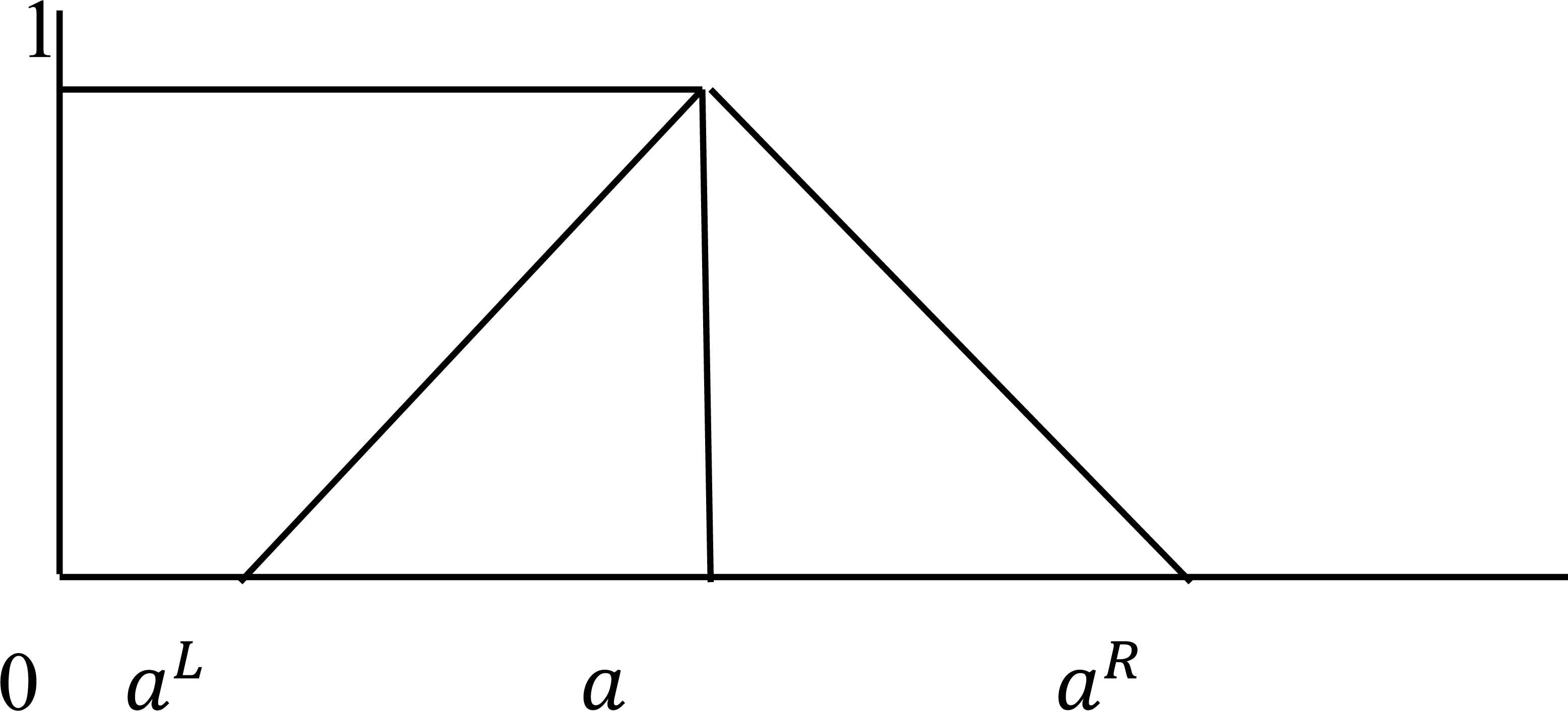
The triangular fuzzy number
Also, there are other types of fuzzy numbers as right sided fuzzy number, left sided fuzzy number, trapezoidal fuzzy number, etc.
2.2 α-cuts
Given a fuzzy set A, its α-cut A[α] is defined as
By definition α-cut A[α] of the fuzzy number à is actually a close interval of real numbers, i.e.,
2.3 First Decomposition Theorem on Fuzzy Sets
Every fuzzy set A defined on Y, the universal set of discourse, can be represented in the form A = ∪α∈[0,1] αA, where the special fuzzy set αA is defined by the membership values αA = α · A[α]; the union is considered as the standard fuzzy union and A[α] represents the α-cut of A.
2.4 Uncertain probabilities
In probability distribution, if one or more parameters are not known precisely and are modeled by using fuzzy numbers are known as uncertain probability. Using fuzzy arithmetic, basic laws of uncertain probabilities can be developed [47].
Let X be a continuous random variable with probability density function f(x,v), where v is a parameter describing the density function. If v is considered as fuzzy number ṽ, then X becomes a fuzzily described random variable with density f(x,ṽ), and the event P(c ≤ X ≤ d) become a fuzzy set whose α-cut is defined as
The first two moments are also defined by their α-cuts as for all α ∈ (0, 1],
Also the FRVs Xi, (i = 1, 2,…, n) having joint density function
2.5 FRVs
An FRV on a probability space (Ω, Φ, P) is a fuzzy valued function X: Ω → Φ0(ℝ), ω → Xω such that for every Borel set 𝔅 of ℝ and for every α ∈ (0, 1], (X[α])−1(𝔅) ∈ Φ. Here Φ0(ℝ) denotes the space of all piecewise continuous functions defined on ℝ. For the set of fuzzy numbers, the set valued function X[α]: Ω → Φ0(ℝ),ω → Xω[α] = {x ∈ ℝ|Xω(x) ≥ α}
By decomposition theorem of fuzzy numbers it is stated that if
3. Formulation of FMOCCP model
An FMOCCP model having K number of objectives having some fuzzily described constraints and some fuzzy chance constraints where the right sided parameters are fuzzily described normally distributed random variables, is presented as
ãij, ũij and ṽi, i = 1,2,…,m;
j = 1, 2,…, n are fuzzy numbers and
4. FP model construction
In this section the fuzzy probabilistic constraints are converted into fuzzy constraints using CCP technique for normal probability distribution.
Let the mean
Therefore, (2) takes the form
The inequality is satisfied only if
Hence
Now, applying first decomposition theorem on fuzzy sets, the constraints in (4) takes the form as
With the help of above fuzzy constraints defined in (5) the following FP model is constructed in the next subsection.
Considering the constraints defined in (5) the model described in (1) takes the form as
Now, in the current decision making situation, the parameters ãij, ũij; mean
Also, the parameters ṽi; i = 1, 2,…,m associated with the fuzzy constraints can be considered as right sided or left sided fuzzy numbers according to “≤” or “≥” inequality which represented by Fig. 2, and Fig. 3, respectively.
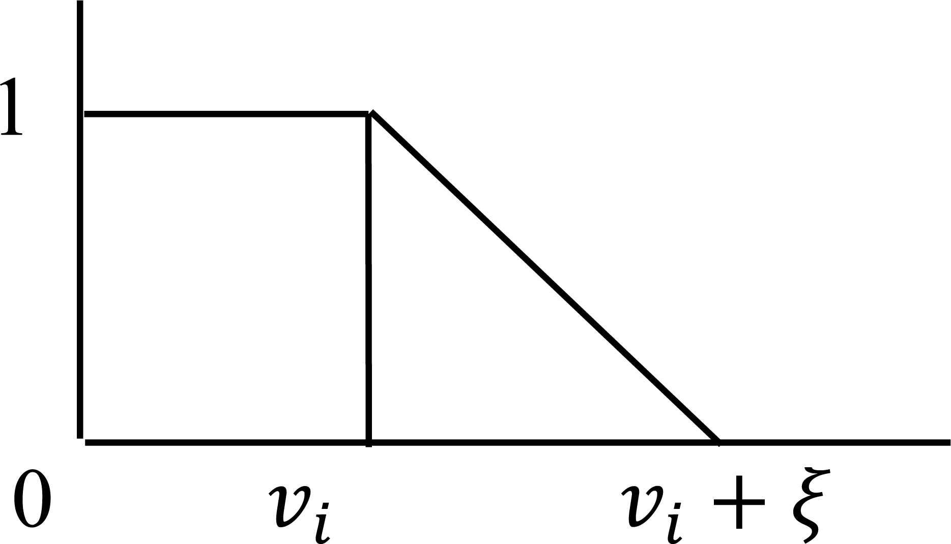
Right sided fuzzy numbers (RSFN)
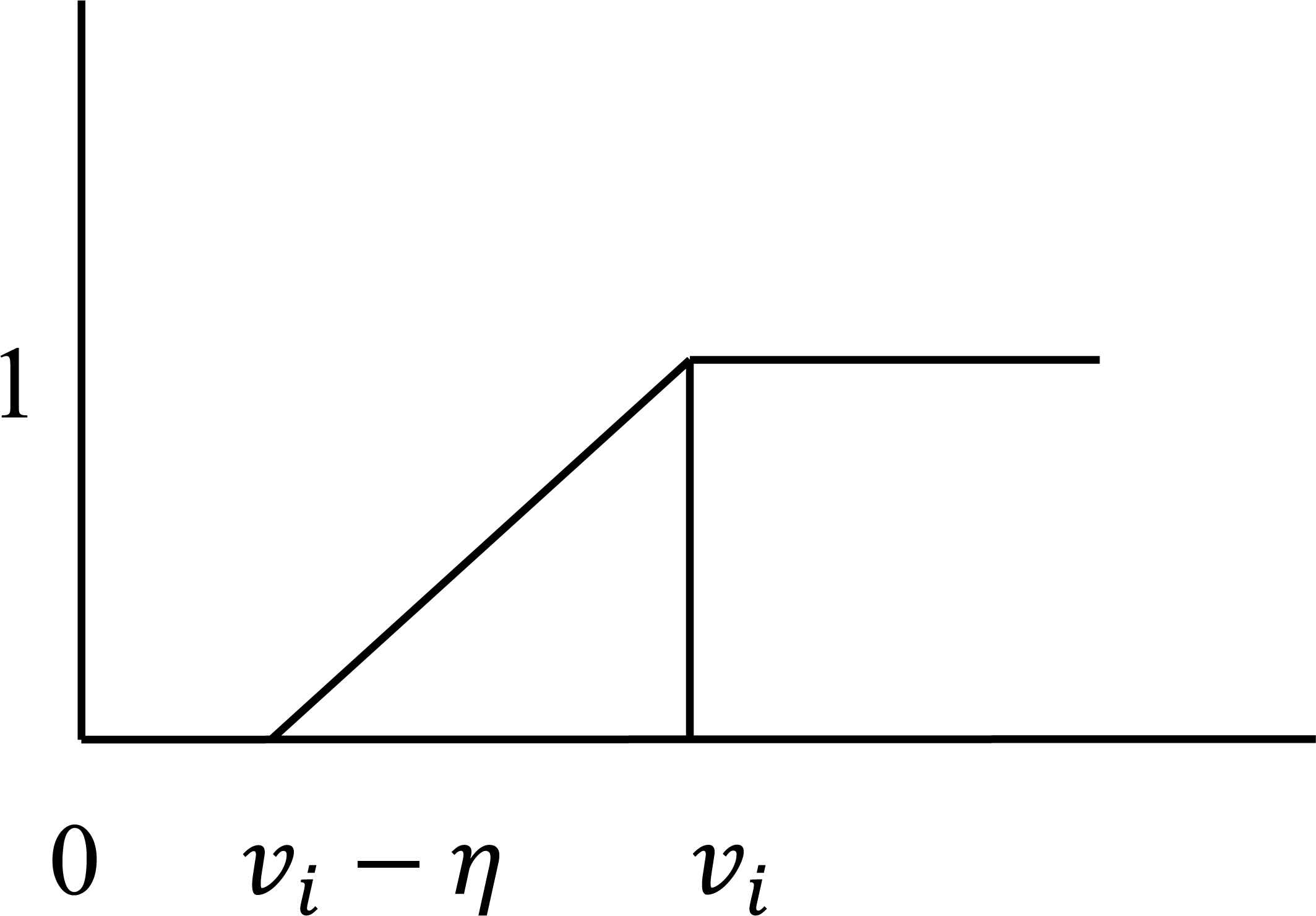
Left sided fuzzy numbers (LSFN)
On the basis of tolerance ranges of fuzzy numbers, the system constraints in (6) are decomposed as
Now, each of the objectives is solved in isolation under the decomposed set of system constraints defined in (7), to define the aspiration level of each of the fuzzy objective goals in the decision making situation. Let
5. Construction of membership functions
In a fuzzy decision making situation, the fuzzy goals are characterized by their membership function with the defined tolerance limits for achievement of their aspired goal levels. The membership function for the defined fuzzy goals can be constructed as
6. Weighted FGP model
The aim of the DMs is to achieve the highest membership value of each of the associated fuzzy goals. But in real life situation, it is not possible to achieve all the ideal membership values, simultaneously, due to limitation of resources. In such a situation FGP technique is used for achievement of the highest membership value of each fuzzy goal of the objectives to the extent possible in decision making environment.
The weighted FGP model of the problem (7) is presented as
where
To assess the relative importance of the fuzzy goals some numerical weights, Mk1, Mk2 (k1 = 1, 2,…, K1; k2 = K1 + 1, K1 + 2,…, K2), are assigned together with the fuzzy weights, Wk1, Wk2 (k1 = 1, 2,…, K1; k2 = 1, 2,…, K2), which are given by
7. FMOCCP model formulation for land allocation problems
The different decision variables and parameters which are associated to represent the model are defined in the following section.
7.1 Nomenclature
7.1.1 Definition of decision variables and parameters
- xcs:
The allocation of land for cultivating the crop c during the season s,
c = 1, 2,…, C; s = 1, 2,…, S
- Pcs :
Estimated production of the crop c per hectares (ha) during the season s.
- Ecs:
Estimated expenditure for cultivating the crop c during the season s.
- Ãs:
Total farming land (hectares (ha)) in use for cultivating the crops during the season s.
Total machine hours (in hrs.) required during the season s.
Total man days (in days) required during the season s.
The Total amount of fertilizer t required (t = 1, 2,…, T) during the planning year.
Total supply of water (in inch/ha) available during the season s.
Average machine hours (in hrs.) required per ‘ha’ for the crop c during the season s.
Average man-days required per ‘ha’ for the crop c during the season s.
Average amount of fertilizer t required per ‘ha’ for the crop c during the season s.
Estimated amount of water consumption (inch/ha) for the crop c during the season s.
Estimated minimum land allocation for the crop c during the season s.
7.2 FMOCCP model construction for land allocation
On the basis of the defined variables and parameters the following FMOCCP model is presented as
The above FMOCCP model is converted into a FP model by the methodology developed in Section 4. Therefore, the FP model corresponding to the model (10) is written as
Now, in the context of land allocation the total farming land available for cultivating all the crops during a season, i.e., Ãs are considered as right sided fuzzy number with aspiration level As and corresponding tolerance limits ξs, s = 1, 2,…, S. The membership functions are defined as follows
Also, the estimated machine hours, man-days for cultivating the crop c during the season s, i.e.,
Similarly, the membership functions for
The membership function for
Let
Then the FP model under the set of decomposed system constraints is presented as
Now, the FGP model corresponding to the problem in (12) is constructed by the methodology developed in section- 7 and solved to find the optimal land allocation.
8. An illustrative example: A case study
8.1 Data description
The land utilization planning for production of the principal crops in the district Nadia of the state West Bengal, India is considered to illustrate the proposed methodology. The available data for the planning years: 2008-2009, 2009-2010, 2010-2011, 2011-2012, 2012-2013 were collected from different sources of agricultural planning units [48 – 50]. During a planning year there are three seasonal crops-cycles; viz. pre-kharif, kharif and Rabi successively appear in the state West Bengal.
The detail of main crops growing in various season with durations are given in the following Fig. 4.

Seasons cycle in West Bengal, India
To develop the FMOCCP model the decision variables and different types of data involved with the problem are given in Table-1 and Table - 2.
| Season (s) | Pre-Kharif (1) | Kharif (2) | Rabi (3) | ||||||||
|---|---|---|---|---|---|---|---|---|---|---|---|
| Crop (c) | Jute (1) | Sugarcane (2) | Aus (3) | Aman (4) | Sugarcane (2) | Boro (5) | Wheat (6) | Mustard (7) | Potato (8) | Lentil (9) | Sugarcane (2) |
| Variable (xcs) | x11 | x21 | x31 | x42 | x22 | x53 | x63 | x73 | x83 | x93 | x23 |
The decision variables representing the seasonal crops
| Crop | Production (Kg/ha) | Expenditure (INR/ha) |
|---|---|---|
| Jute | 2717.81 | 17430 |
| Sugarcane | 67676.87 | 30922 |
| Aus | 3979.79 | 14500 |
| Aman | 4644.06 | 14000 |
| Boro | 5625.98 | 25000 |
| Wheat | 33093.73 | 12000 |
| Mustard | 1240.62 | 8700 |
| Potato | 25218.35 | 35932 |
| Lentil | 1316.97 | 6500 |
Production and expenditure of various crops during 2012 – 2013
The variables x21, x22, x23 represent the same decision variable, since the cultivation of sugarcane runs throughout the year.
The total farming land, total machine hours and total man-days are required in a season for the years 2010-2011, 2011-2012, and 2012-2013 [48, 49], which are presented in Table- 3.
| Season (s) | Total farming land (’000 ha) | Total Machine-hours (in hrs) | Total Man-days (in days) | ||||||
|---|---|---|---|---|---|---|---|---|---|
| 2010-11 | 2011-12 | 2012-13 | 2010-11 | 2011-12 | 2012-13 | 2010-11 | 2011-12 | 2012-13 | |
| Pre-Kharif | 292.32 | 305.33 | 295.32 | 13999.6 | 14443.4 | 15124.2 | 14256 | 14289.1 | 14281.1 |
| Kharif | 288.56 | 293.36 | 272.96 | 7335.45 | 7122.23 | 7299.56 | 6502 | 6535.1 | 6501.2 |
| Rabi | 305.23 | 299.54 | 307.12 | 35362.2 | 35383.5 | 35371.6 | 11325 | 11302.1 | 11313.5 |
Data description regarding productive resources
From the available data it is observed that the total farming land, total machine hours and total man-days which are required for a season varies in different planning years. So, these three productive resources described above are considered as fuzzy numbers which are represented in Table–4 with their respective tolerance limits.
| Season (s) | Total farming land (in ’000 ha) (RSFN) | Total Machine- hours (in hrs) (LSFN) | Total Man-days (in days) (LSFN) | |||
|---|---|---|---|---|---|---|
| As | ξs | Hs | ηs | Ds | ζs | |
| Pre-Kharif | 300 | 10 | 14522.30 | 1452.23 | 14274.1 | 1427.41 |
| Kharif | 300 | 10 | 7253.57 | 725.35 | 6513.1 | 651.31 |
| Rabi | 300 | 10 | 35373.01 | 3537.30 | 11312.2 | 1131.22 |
Data description for productive resources
In the context of utilizing productive resources, it is worthy to mention here that the average machine hours and average man-days, which are required per ‘ha’ for various crops are considered as fuzzy numbers since they are also varied for different planning years. For example, from the available data it is clear that in Pre-Kharif season the machine hours required per ‘ha’ for cultivating Jute vary in between 64 to 68 hours. So, it is considered as a triangular fuzzy number as (64, 66, 68). Similarly, other fuzzy numbers corresponding to average machine hours and average man-days in different seasons and for different crops have been defined and presented in Table – 5.
| Crops | Average Machine hours (in hrs/ha) | Average Man-days (in days/ha) |
|---|---|---|
| Jute | (64, 66, 68) | (88, 90, 92) |
| Sugarcane | (56, 58.2, 60.4) | (39, 41, 43) |
| Aus | (136, 139, 142) | 957, 60, 63) |
| Aman | (64, 66, 68) | (58, 60, 62) |
| Boro | (262, 267, 272) | (58, 60, 62) |
| Wheat | (65.5, 66, 66.5) | (38, 39, 40) |
| Mustard | (33, 33.5, 34) | (28, 30, 32) |
| Potato | (109, 112, 115) | (67, 70, 73) |
| Lentil | (48.5, 49, 49.5) | (14, 15, 16) |
Data description for utilization of resources
Nowadays, there is an increasing emphasis of using compost for maintaining the soil quality of the cultivating lands by the cultivator, so they might not use common fertilizer for a season for some crops, but the supply of compost is not sufficiently available throughout the years due to the lack of awareness of the people for preparing and utilizing compost. So, the common fertilizer requirement is probabilistic in nature. Since the productions of different crops are not precise in nature the requirement of common fertilizers [51] varies in different planning years. So, in Table – 6, the total requirements of fertilizer are not only probabilistic but also possibilistic which are represented in term of FRVs with imprecise mean and variance.
| Fertilizer
|
2010-11 (’000mt) | 2011-12 (’000mt) | 2012-13 (’000mt) |
|
|
|---|---|---|---|---|---|
| Nitrogen (N) |
|
|
|
|
|
| Phosphate (P) |
|
|
|
|
|
| Potash (K) |
|
|
|
|
|
Data description for requirement of fertilizer
It is also realized from the data available for the previous years that the utilization of fertilizers per ‘ha’ and consumption of water (inch/ha) for various crop is imprecise in nature, which are represented in Table – 7, in terms of triangular fuzzy numbers.
| Crops | N (Kg/ha) | P (Kg/ha) | K (Kg/ha) | Water consumption (inch/ha) |
|---|---|---|---|---|
| Jute | (36, 39, 42) | (18, 20, 22) | (17.5, 19.5, 21.5) | (19.5, 20, 20.5) |
| Sugarcane | (175, 200, 225) | (66, 110.5, 105) | (90, 100, 110) | (57.5, 60, 62.5) |
| Aus | (39, 41, 43) | (20, 20.5, 21) | (20, 21, 22) | (32.2, 34, 35.8) |
| Aman | (36, 36.5, 37) | (18, 19, 20) | (20, 21, 22) | (47.8, 50, 50.2) |
| Boro | (100, 110, 120) | (47, 51, 55) | (47, 51, 55) | (69.2, 70, 70.8) |
| Wheat | (100, 110, 120) | (55, 57.5, 60) | (55, 57.5, 60) | (14.8, 15, 15.2) |
| Mustard | (80, 83, 86) | (40, 41, 42) | (40, 41, 42) | (9.6, 10. 10.4) |
| Potato | (135, 150, 165) | (70, 77.5, 85) | (70, 77.5, 85) | (17.3, 18, 18.7) |
| Lentil | (20, 22.5, 25) | (60, 62.5, 65) | (25, 27, 29) | (9.5, 10,10.5) |
Data description for utilization of fertilizer and consumption of water in the year 2012-2013
It is to be noted here that total water supply in various seasons depends largely on environmental conditions. The total water supply partially depends on rainfall in a season, which is probabilistic in nature. Also, there might have some alternative sources of water used by the cultivators for various crops during a season for more production, which are imprecisely defined. So the total water supply is not only probabilistic in nature, but imprecision involved inherently within it. Therefore, the total water supply in various seasons is considered as FRVs where the mean and standard deviation are considered as triangular fuzzy numbers as shown in Table – 8.
| Water supply | 2009-10 (inch/acre) | 2010-11 (inch/acre) | 2011-12 (inch/acre) | 2012-13 (inch/acre) |
|
|
|---|---|---|---|---|---|---|
| Pre-Kharif |
|
|
|
|
|
|
| Kharif |
|
|
|
|
|
|
| Rabi |
|
|
|
|
|
|
Data description for supply of water
From the available data it is evident that a minimum level of land is allocated for a crop during a season, which is calculated and presented in Table – 9 with their tolerance limit.
| Crops | Minimum land required (RSFN) (‘000 ha) |
|
|---|---|---|
| Amin | τ | |
| Jute | 139 | 16 |
| Sugarcane | 1.5 | 1 |
| Aus | 43 | 15 |
| Aman | 92 | 8 |
| Boro | 80 | 10 |
| Wheat | 57 | 5 |
| Mustard | 110 | 10 |
| Potato | 25 | 3 |
| Lentil | 30 | 5 |
Minimum level of land utilization for various crops
8.2 FMOCCP Model
Now, based on the data presented in Table 1–9, the following FMOCCP model is constructed.
Objectives:
Constraints:
Land allocation constraints
Machine hour’s constraints
Man-days constraints
Fertilizer utilization constraints (N, P, K respectively)
Water utilization constraints
Minimum level of land utilization constraints
Now, the system constraints in (13) are decomposed on the basis of the fuzzy numbers associated with the constraints in the decision making context as described in (12).
Then solving the objectives individually with respect to the system constraints derived from (13) the best and worst objective values are found as
Afterwards, the membership function of the objectives is constructed as defined in (8).
Now, the FGP model is constructed as defined in section-7 and is solved by using software version Lingo (11.0) for finding the optimal cropping plan in the current agricultural planning environment.
9. Results and discussions
On solving model (14) the following solutions are achieved which are presented in Table – 10.
| crop | Jute | Sugarcane | Aus | Aman | Boro | Wheat | Mustard | Potato | Lentil |
|---|---|---|---|---|---|---|---|---|---|
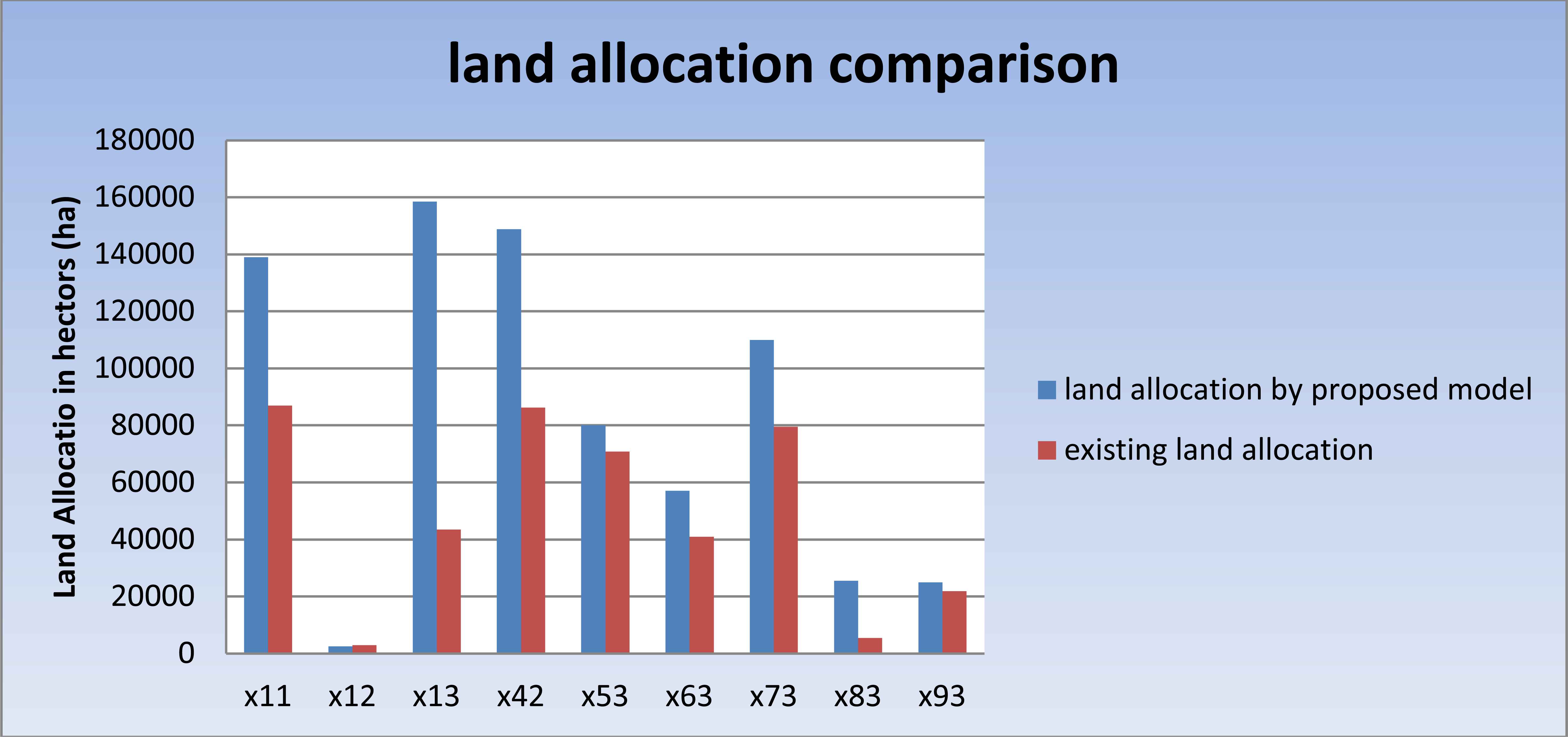
| Land Allocation | 139000 | 2500 | 158500 | 148750 | 80000 | 57000 | 110000 | 25500 | 25000 |
| Production (’000mt) | 377.78 | 101.52 | 630.79 | 690.80 | 450 | 188.65 | 136.47 | 643.07 | 32.92 |
Achieved land allocation and production using proposed model
The existing land allocation and production in the planning period 2012-2013 is presented in Table –11.
| crop | Jute | Sugarcane | Aus | Aman | Boro | Wheat | Mustard | Potato | Lentil |
|---|---|---|---|---|---|---|---|---|---|
| Land Allocation | 86875 | 2940 | 43500 | 86250 | 70800 | 40900 | 79500 | 5450 | 21800 |
| Production (’000mt) | 236.11 | 198.97 | 173.12 | 400.55 | 398.32 | 135.37 | 98.63 | 137.44 | 28.71 |
Existing land allocation and production in the planning year 2012-2013
Further, considering fuzzy equivalent crisp numbers of the problem, the model is solved using goal programming. The achieved land allocation and production is presented in Table - 12.
| crop | Jute | Sugarcane | Aus | Aman | Boro | Wheat | Mustard | Potato | Lentil |
|---|---|---|---|---|---|---|---|---|---|
| Land Allocation | 139000 | 1500 | 43000 | 92000 | 80000 | 57000 | 110000 | 22000 | 20000 |
| Production (’000mt) | 377.78 | 60.92 | 171.13 | 427.25 | 450.08 | 188.66 | 136.47 | 554.8 | 26.34 |
Achieved land allocation and production using goal programming
A pictorial diagram representing a comparison between the achieved land allocation through the proposed model and the existing land allocation in the planning period 2012-13 is presented in Fig. 5.
Comparison between the proposed model and the existing land allocation
It is evident from the Fig. 5 that the proposed model provides more scientific and better land allocation in a planning year for various crops.
Fig. 6 represents a comparison between the production achieved through the proposed model and the production received through the existing cropping plan (2012 – 13).
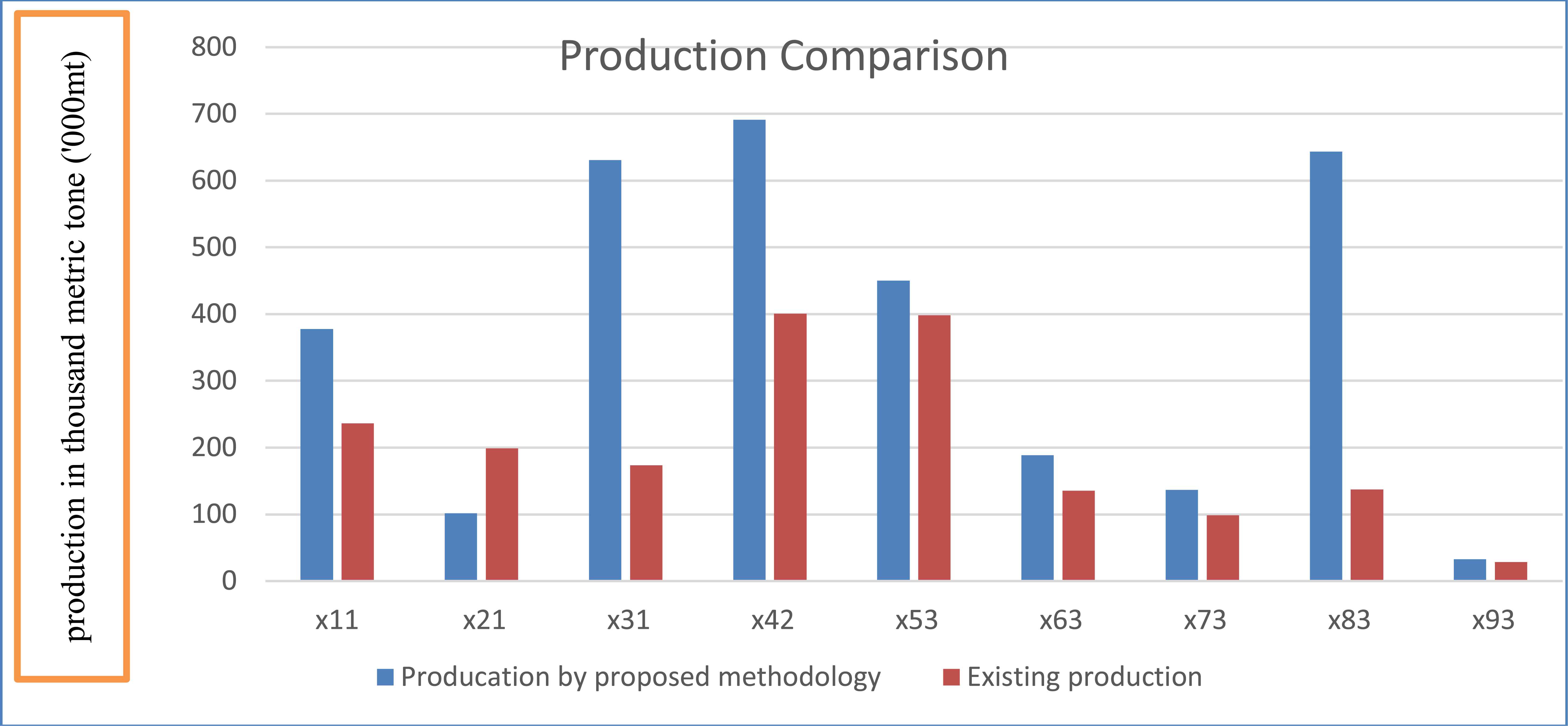
Comparison of production achieved using the proposed model and with the production in 2012 -13.
Fig. 7 depicts a pictorial diagram for comparing production achieved via the proposed methodology, GP methodology and the existing cropping plan.

Comparison of production using the proposed methodology, using goal programming and existing production.
The comparison shows that a better cropping plan is obtained using the proposed methodology from the viewpoint of achieving maximum production by utilizing maximum land available in a planning year. The annual expenditure is found as INR 11,600,591,000/- through this proposed model, but the expenditure in 2012-13 was INR 6,733,371,330/-. The expenditure is increased here because the production is much higher than the original production. In this context, it is also to be noted that, the total annual income from existing production is INR 31,863,574,000/-, on the other hand the total annual income will be INR 53,094,249,500/- by the proposed methodology. Therefore, the annual income increased significantly by the proposed methodology. The profit from existing land allocation and production is INR 25,130,202,670/-, but the profit can be achieved INR 41,493,658,500/- by the proposed model. Therefore, total profit increased by an amount INR 16,363,455,830/-.
10. Conclusions
In the framework of the proposed methodology, different parameters in the forms of either fuzzy or probabilistic or the both associated with the problem can easily incorporate without any computational difficulties. An optimal cropping plan for allocation of lands under cultivation from the viewpoint of maximizing the total production and minimizing the expenditure of cultivation has been achieved under the proposed framework. Through this model a better cropping plan has been found in terms of utilizing land and achievement of total production. The output of this research may become a useful tool for agricultural planners, who are using the traditional methods for recommendations to the farmers on optimal land allocation for different seasonal crops in the planning process. Finally, it is hoped that the solution procedure presented here can contribute to the future studies in farming and other fuzzy stochastic MODM problems in the current uncertain decision making atmosphere.
Acknowledgements
The authors remain grateful to Department of Agri-irrigation, Office of the executive Engineer, Krishnagar, Nadia, Govt. of West Bengal, India for active support in supplying data to implement the case study of the developed model. The authors are thankful to the reviewers for their valuable comments and insightful suggestions for improving the quality of the article.
References
Cite this article
TY  - JOUR
AU  - Animesh Biswas
AU  - Nilkanta Modak
PY  - 2017
DA  - 2017/01/01
TI  - A Multiobjective Fuzzy Chance Constrained Programming Model for Land Allocation in Agricultural Sector: A case study
JO  - International Journal of Computational Intelligence Systems
SP  - 196
EP  - 211
VL  - 10
IS  - 1
SN  - 1875-6883
UR  - https://doi.org/10.2991/ijcis.2017.10.1.14
DO  - 10.2991/ijcis.2017.10.1.14
ID  - Biswas2017
ER  -