
Times Series Forecasting using Chebyshev Functions based Locally Recurrent neuro-Fuzzy Information System
- DOI
- 10.2991/ijcis.2017.10.1.26How to use a DOI?
- Keywords
- Recurrent neuro-fuzzy network; Chebyshev polynomials; TSK fuzzy rules; Firefly-Harmony search algorithm; electricity price forecasting; currency exchange rate prediction; stock indices prediction
- Abstract
The model proposed in this paper, is a hybridization of fuzzy neural network (FNN) and a functional link neural system for time series data prediction. The TSK-type feedforward fuzzy neural network does not take the full advantage of the use of the fuzzy rule base in accurate input-output mapping and hence a hybrid model is developed using the Chebyshev polynomial functions to construct the consequent part of the fuzzy rules. The model to be known as locally recurrent neuro fuzzy information system (LRNFIS) is used to provide an expanded nonlinear transformation to the input space thereby increasing its dimension which will be adequate to capture the nonlinearities and chaotic variations in the time series. The locally recurrent nodes will provide feedback connections between outputs and inputs allowing signal flow in both forward and backward directions, giving the network a dynamic memory useful to mimic dynamic systems. For training the proposed LRNFIS, an improved firefly-harmony search (IFFHS) learning algorithm is used to estimate the parameters of the consequent part and feedback loop parameters. Three real world time series databases like the electricity price of PJM electricity market, the widely studied currency exchange rates between US Dollar (USD) and other four currencies i.e. Australian Dollar (AUD), Swiss Franc (CHF), Mexican Peso (MXN), Brazilian Real (BRL), along with S&P 500 and Nikkei 225 stock market data are used for performance validation of the newly proposed LRNFIS.
- Copyright
- © 2017, the Authors. Published by Atlantis Press.
- Open Access
- This is an open access article under the CC BY-NC license (http://creativecommons.org/licences/by-nc/4.0/).
1. Introduction
List of important symbols
- µ
membership function
- c, σ
centre and spread of the fuzzy set
- λ
Locally recurrent feedback parameter
- ω, ϕ
weight and chebyshev polynomial functions, respectively
- rij
Cartesian distance between ith and jth fireflies
- β
attractiveness value between two fireflies
- α
random movement factor
- k, K
iteration count, maximum number of iterations, respectively
- HM
harmony memory
- HMCR
harmony memory consideration rate
- PAR
pitch adjustment rate
- BW
pitch adjustment bandwidth
- U,L
upper and lower bound of the variables
- rand
random number between 0 and 1
Time series forecasting has a wide range of applications in finance, signal processing, electric load forecasting, weather forecast, hydrological prediction, sunspot prediction, condition monitoring of equipments for alarm processing, and electricity price prediction in energy markets, etc. Most of the time series data that occur in financial and engineering fields are chaotic in nature and exhibit nonstationary behavior amounting to chaotic fluctuations. Significant research efforts have been undertaken to mine these highly chaotic time series databases in the way of either forecasting or classifying patterns in the database.
Many techniques have been employed over the years for time series forecasting purpose, including statistical methods like Autoregressive Moving Average (ARMA), Autoregressive Integrated Moving Average (ARIMA), and Generalized Autoregressive Conditional Heteroskedasticity (GARCH) models [1–5], intelligence techniques like artificial neural networks (ANNs) [6–11], fuzzy inference system (FIS) [12–15], and support vector machines (SVMs) [16–20], etc. Moreover, time series models like ARIMA, and GARCH, have also been proven to be effective in the stock and electricity price forecasting/modeling. However, for short-term forecasts, Artificial Neural Networks (ANNs) are flexible computing frameworks and universal approximators that can be applied to a wide range of time series forecasting problems with a high degree of accuracy. According to a recent study, the machine learning methods (ANNs, SVMs) outperform other time series methods (ARMA, GARCH) due to their superior handling capacity of the chaotic behavior of the time series databases. Due to the generalization capabilities and robustness, the ANN is extensively used in various time series forecasting.
Among other neural network models; Radial Basis Function Neural Network (RBFNN) [21–23], Local Linear Radial Basis Function Neural Network (LLRBFNN) [24], Wavelet Neural Network (WNN) [25], Local Linear Wavelet Neural Network (LLWNN) [26–27], Recurrent Neural Network (RNN) [28–29], are widely used in time series prediction. Further to meet the increasing needs for better forecasting models; several nonlinear models have been developed by researchers. Fuzzy Logic theory [30–34] has found to be suitable in many applications as these methods are suitable due to their superior abilities in the handling of non probabilistic uncertainties that occur in financial and energy markets. Adaptive Neural Network based Fuzzy Information Systems (ANFIS) [35–39] and Fuzzy Neural Networks (FNN) work successfully in many time series forecasting problems.
Time series forecasting accuracy is an important yet often difficult task faced by the researchers in many real world problems. Numerous theoretical and empirical studies have confirmed that hybridized models can be an effective way for improving the accuracy of the forecast. Each model can capture certain characteristics hidden in the data and contribute effectively in improving the overall forecasting performance. A single model may not be able to capture all the uncertainties in the time series and therefore may not be able to predict the futuristic behavior of the time series accurately. Thus the hybridization of statistical models like ARMA, ARIMA or GARCH with feedforward neural networks [40–41] is used widely for time series forecasting especially in financial and energy price time series databases. In recent years, more hybrid forecasting models have been proposed using feed-forward neural networks and applied in many areas with good prediction performance. Among the various hybrid models, like the Fuzzy information systems with ARIMA [42–43], Fuzzy wavelet neural networks with GARCH [40], etc. have been successfully applied in time series prediction.
Although there are several studies that involve fuzzy inference systems, and neuro-fuzzy inference systems for financial time series prediction, there is hardly any substantial research in the application of recurrent neuro-fuzzy inference systems for predicting highly chaotic nonlinear times series like financial or electricity market data. Normally the recurrent structure in the network is introduced either in the firing strength layer or in output and input layers and so on. Thus in this research, a new locally recurrent neuro-fuzzy inference System (LRNFIS) is presented that includes a feedback loop in the firing strength layer to memorize the temporal nature of the fuzzy rule base and provide a dynamic nature to the time series forecasting problem.
In the widely used neuro-fuzzy information systems, the consequent part of the fuzzy rule base is of the TSK-type that has more free parameters to adjust providing a better input-output mapping. However, the TSK-type feedforward recurrent fuzzy neural network does not take the full advantage of the use of the fuzzy rule base in approximating functions and therefore a hybridization procedure is adopted by using Chebyshev polynomial functions to construct the consequent part. The Chebyshev polynomial function model will provide an expanded nonlinear transformation to the input space thereby increasing its dimension which will be adequate to capture the nonlinearities and chaotic variations in time series prediction problems. Further hybridizing it with recurrent fuzzy neural information system will result in a significant convergence and accuracy in time series prediction. It is well known that the weight parameters of the fuzzy neural information systems are normally trained by gradient descent, recursive least squares, extended and unscented Kalman filters and most of these algorithms suffer from slow convergence and high computational overhead. To circumvent these problems metaheuristic evolutionary algorithms like Firefly [44–46] and Harmony search [47–50] are hybridized to estimate the parameters of the weights associated with TSK Fuzzy rule base and locally recurrent feedback loops. The hybridization is done primarily to overcome the local search problems associated with the conventional Firefly algorithm and the improved hybrid version (IFFHS) provides better diversity, speed of convergence, and forecasting accuracy. The proposed LRNFIS model is compared with the well known RBFNN trained by the same IFFHS metaheuristic evolutionary algorithm for the prediction of PJM electricity market prices time series. Further, financial time series databases like currency exchange rate time series and stock time series are taken for prediction over a time frame varying from one day to several days ahead to prove the validity of the proposed LRNFIS model.
The paper is organized in 7 sections. Section 2 presents the TSK fuzzy rule based LRNFIS model and its training algorithm comprising the IFFHS algorithm is presented in section 3. Section 4 provides performance matrix whereas section 5 presents applications to predict the PJM electricity market, AUD/USD, CHF/USD, MXN/USD, and BRL/USD currency exchange rate, and S&P 500 and Nikkei 225 stock market time series databases. Finally conclusion is presented in section-6.
2. TSK fuzzy rule based LRNFIS model used for Time Series prediction
This section presents the structure of the LRNFIS where the firing strength of each rule is locally fed back to itself creating a locally recurrent fuzzy system. The locally recurrent structure of the LRNFIS provides memory to the learning paradigm thereby capturing the dynamic behavior of the highly fluctuating time series databases. The consequent part of each recurrent fuzzy rule has a first order TSK-type built around Chebyshev polynomial basis functions. The LRNFIS comprises seven layers and is depicted in Fig.1. Different layers of the LRNFIS perform different mathematical functions which are described below:
Layer 1 (Input Layer):
This layer contains the input data comprising the past values of the time series are directly transmitted to the next layer which is a fuzzification layer.
Layer 2 (Fuzzification Layer):
In this layer the input data is fuzzified using a suitable Gaussian membership function for the fuzzy set Aij as:
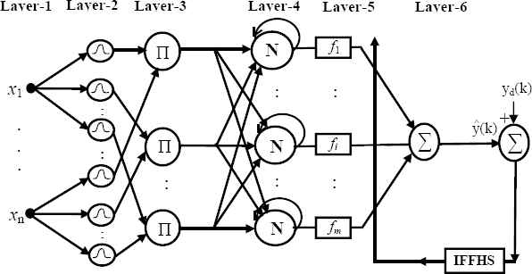
Locally recurrent neuro-fuzzy information system (LRNFIS)
Layer 3 (Spatial Firing Layer):
Here each node functions as a spatial rule node corresponding to each TSK type fuzzy rule, which is described in the following form:
Thus, the firing strength of the jth fuzzy rule is obtained with the help of product T-norm of the antecedent fuzzy sets as
Layer 4 (Normalization and locally recurrent layer)
Each node output in this layer is a normalized temporal firing strength, which is obtained from the ratio of the jth rule’s temporal firing strength to the sum of all rules’ temporal firing strengths as follows:
Layer 5 (Consequent Layer):
The consequent layer is a layer of adaptive nodes which comprises the TSK rule base using Chebyshev polynomial basis function and its output is obtained as
The higher order Chebyshev Polynomials can be generated using the generalized recursive formula given in equation (9)
Thus comparing equations (8) and (9)
Layer 6 (Output Layer):
In this layer, the overall output of the LRNFIS is calculated as the summation of the rule consequences as follows:
The performance of the proposed LRNFIS model mainly depends on fine tuning of the antecedent, consequence, internal feedback weights for highly fluctuating time series databases.
3. Training Algorithm for the LRNFIS
In this paper, a hybrid learning paradigm is used for LRNFIS to obtain the parameters of the fuzzy sets. A clustering approach is used to initialize the centre and spread (cij and σij) of the fuzzy membership values after they are updated using a gradient descent algorithm. However, for updating the weights associated with the local recurrent outputs and the consequent parts of the TSK fuzzy rules; the first step is known as the structure learning and the second step is designated as the weight parameter learning.
Step 1: Structure Learning
To obtain the updated fuzzy membership parameters, an error cost function E(k) is formulated as
Using the above error cost function and gradient descent rule the parameter adjustment is done as follows:
On simplification we obtain
Step 2: TSK and locally recurrent feedback loop weight parameter learning
It is well known that the evolutionary algorithms yield global optimized solutions for many multimodal real world problems and hence this paper presents a hybrid Firefly and differential Harmony search algorithm for parameter tuning of the TSK type fuzzy rule base. Firefly algorithm (FA) originally proposed by Xin-She Yang and others [44–46] is a metaheuristic algorithm which is based on the flashing behavior of the fireflies. The flashing light is produced by a chemical reaction known as the bioluminescence, and has a short and rhythmic characteristic. The flashing light of the fireflies is considered as a signaling system to attract other fireflies and warn the predators. As fireflies are unisex one firefly can be attracted to the other one depending on its brightness, which is measure of higher value of the objective function. Despite being an effective optimization tool, FA proposed by Yang, [45] has difficulty of randomization between global solution and local search and thus an improved Harmony search (HS) [47–50] is adopted with conventional FA to overcome the drawback of randomness by increasing diversity in firefly population. The HS algorithm is a relatively new metaheuristic search algorithm originally conceptualized from musical instruments which depends on the operators like the harmony memory (HM) and its size (HMS), the harmony memory consideration rate (HMCR), the pitch adjustment rate (PAR), and the pitch adjustment bandwidth (BW). Further, the value of each decision variable in HS optimization algorithm is determined by the three parameters HMCR, PAR, and BW. In this paper, the error cost function in equation (17) is chosen as the objective function for initiating the search process.
The parameters of the model have been estimated by minimizing the root mean square error (RMSE) criterion. Therefore, the objective function for optimization is defined as:
Step 3: Firefly Algorithm (FF) for Weight parameter estimation of the LRNFIS
Initially ‘N’ no. of fireflies are declared for ‘D’ dimensions randomly. The number of dimensional field is the number of decision variables, which is again the number of TSK Legendre basis functions associated parameters to be estimated along with the recurrent path gain parameters. The randomized range of these decision variables is assumed and the final expression of solution vector (X) is:
The attractiveness value β between any two fireflies i and j varies with the Cartesian distance rij between them and is obtained as
According to the concept of global optima, the fireflies with minimum light intensity are opted as best fireflies (xgbest) for that particular generation. Instead of comparing each firefly with other fireflies, it is more convenient to compare it with best firefly to reduce computational complexity. Thus the Eq.(17) is modified by using the global optimization concept as:
Here βmax and βmin are maximum and minimum attractiveness for that generation. The best distance (rij,best) is obtained from equation (25) as
Step 4: Improved Harmony Search algorithm (IFFHS) for better exploration
In the Firefly algorithm, the fireflies having low brightness resulting from local search operation cannot compete with best fireflies which move towards global solutions and therefore are discarded. Thus, all fireflies that do not achieve exploitability with best fireflies are not considered while updating solution vector (X) for the next iteration. Due to this property conventional FA may give erroneous local solutions, and hence an improved harmony search algorithm is considered for those firefly populations to improve their performance by using mutation process. The harmony search approach uses the philosophy of music improvisation, where musician endeavor his musical tune improvisation to achieve optimal harmony. To hybridize the conventional FA, HM vector is the initially declared random position of the fireflies.
To find the improved solution globally as well as locally, HMCR and PAR are the two responsible parameters. For conventional HS, more number of iterations are required to find optimal solution, due to consideration of fixed valued PAR and its BW. For this improved HS, during improvisation of new harmony, both PAR and HMCR are expressed as linear incremental function and BW is obtained as exponentially decreasing function.
The PAR is linearly varied by using the equation:
In a similar way the HMCR is varied as
The pseudo code for proposed improved Hybrid Firefly and Harmony search Algorithm (IFFHS) is presented below:
BEGIN
- (1)
The objective of the optimization problem is to minimize the root mean square error E(x) given in eq. (17);
where X is a solution vector comprising the decision variables xi and Ui and Li are the upper and lower bounds for the decision variables, respectively; K =1,2,……….,D; D=number of dimensions=M. - (2)
Initialize different algorithm parameters like, α=randomization parameter, βmax , βmin, PARmax , PARmin, BWmax, BWmin, γ, NI.; NI=number of iterations or generations.
- (3)
Generate initial population of n number of fireflies. Declare random gain matrix XND having value of decision variables within the range.
- (4)
Light intensity Ii is calculated for each Xi which is equal to the fitness function value at Xi by using the root mean square error between the actual and predicted output value.
- (5)
Find the current best solution called as global best solution (Xgbest) and the corresponding function value (Igbest=fgbest).
While k < NI
- ▪
Evaluate pitch adjustment rate (PAR), HMCR, and pitch adjustment bandwidth (BW) using equations (27), (28), (29), respectively.
- ▪
for i=1 to no. of fireflies
If Igbest<Ii
Calculate attractiveness of the fireflies βbest and distance between two fireflies rigbest by using the eq. (24) and eq. (25), respectively.
Move all fireflies (i) towards the least bright firefly (gbest) by using eq. (23).
Else
If rand(0,1)<HMCR Take a variable a= any random integer a ∈ (1, N). We can write it as
Then xi,k = xa,k
If rand(0,1) <PAR
xi,k = xi,k ± rand(0,1) × BW(k)
if f(xi,k ≤ f(xa,k)) then
xa,k = xi,k
End if
End if
Else
xi,k = Li,k + rand(0,1) × (Ui,k − Li,k)
End if
End if
End for
- ▪
- (6)
Check whether the values of the decision variables are within the range or not. If the value of the decision variables is not within the range then the lower limit of that decision variable will be assigned to it.
- (7)
Evaluate the light intensity values of the firefly which will be used for next generation (iteration) using updated parameters.
- (8)
Rank the fireflies according to the light intensity and find the current best solution based on the rank given to the fireflies. Update the global best solution (Xgbest) and the corresponding functional value (Igbest=fgbest).
End of while. (Stopping criteria)
END
4. Performance Metrics
4.1. Various Error Metrics for Prediction Accuracy Evaluation
The Root Mean Square Error (RMSE), Mean Absolute Percentage Error (MAPE) and Mean Absolute Error (MAE) are used to compare the performance of the models for predicting the time series datasets using LRNFIS and IFFHS learning algorithm. To evaluate the performance of the proposed recurrent fuzzy neural system the following error metrics are defined as:
- yk
= actual closing price on kth day
- ŷk
= predicted closing price on kth day
- N
= number of test data.
4.2. Model Performance using Superior Predictive Ability (SPA) test
The forecasting performance of the several models can be assessed in a better way using the Superior Predictive Ability (SPA) test than the error metrics values like MAPE, etc. This test helps to identify whether any of the competing models (m=1, 2….M) is better than the benchmark model in terms of expected loss. For this purpose, the null hypothesis is specified as none of the models is better than the benchmark model against the alternative that among the competing models at least one is significantly better than the benchmark. A supremum over the standardized performance values has been applied by Hansen to test the null hypothesis as:
Using the statistic:
- dm,t
= Lo,t − Lm,t
The loss function at time t for the benchmark model is defined by Lo,t and Lm,t , respectively that indicates the value of the corresponding loss function for another competing model m; n is the no. of out of sample data. The distribution of the test statistics under null hypothesis is approximated by the empirical distribution derived from bootstrap resample based on stationary bootstrap. This is defined as:
Using the three g(x) values, there are three corresponding SPA test values i.e. SPAl, SPAc and SPAu. SPAl represents the lower bound, SPAc represents the consistent value and SPAu represents the upper bound of SPA test statistics. Before calculating P value of SPA test first the SPA statistics for each bootstrap is evaluated in the following manner:
Using the comparison of SPA statistics of each bootstrap with original SPA statistics, the P value of SPA test is obtained as follows:
- B
= total number of bootstraps.
A high pSPA value indicates that the Null hypothesis cannot be rejected, which means that the bench mark model is not outperformed by the competing models. On the other hand a lower pSPA value signifies the rejection of the Null hypothesis clearly indicating the bench mark has been outperformed by other competing models. The upper bound of p-value (SPAu)assumes that all the competing models are precisely as good as the benchmark in terms of the loss function µm (m=1,2,…….,M). On the contrary the lower bound of p-value (SPAl) that the models with worse performance than the benchmark are in fact poor models in the limit. To avoid the data snooping problem, the upper and lower bound of the SPA test over MAPE error has been calculated for the PJM electricity market dataset.
5. Applications of LRNFIS to Real World Time Series Databases
For implementing the proposed LRNFIS to forecast the future values of the time series, a Flow chart is shown in Fig.2. Further to evaluate the performance of the proposed LRNFIS model, three real world time series databases are used. Also for comparison the widely used RBFNN using IFFHS evolutionary algorithm is analyzed to provide the validation of improved performance of the proposed LRNFIS model.

Flow Chart for LRNFIS Implementation
Dataset-1:
The first time series considered for analysis is the electricity price, which is a key issue for all the power market stake holders keeping in view of accurate bidding strategy in the day-ahead power pools. With a proper day-ahead forecasting of electricity prices, the end users or the electricity consumers can minimize their utilization cost and at the same time the generation companies can maximize their daily revenues. The market participants face lots of difficulties to develop their proper business planning with regard to the market clearing prices because of many uncertainties like high spikes in prices, temperature effects, seasonal variations and stochastic nature of demands etc. Because of all these uncertain factors, the price time series in almost all markets exhibits non-stationary means and variances. Several methods that involve both statistical methods like ARMA, ARIMA, and GARCH [3,40,51] models and intelligent system techniques like ANN, FIS, SVM [11,52,53,14,16], etc. have been proposed by researchers for day-ahead electricity price forecasting incorporating different uncertain effects in the deregulated electricity markets.
Before incorporating the electricity price time series data into the proposed model, it is highly essential for the data series to be pre-processed. For this dataset, the single-period continuously compounded return series, known as log-return series is considered for day ahead prediction. The return series has efficient statistical properties and it is easy to handle the highly fluctuating price signals. The single-period continuously compounded return series is defined as:
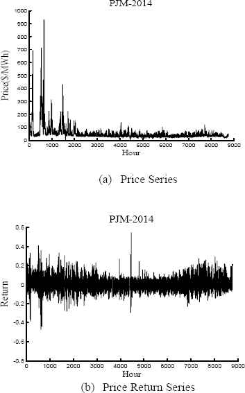
PJM Electricity price and its Return datasets
For highly fluctuating time series the number of lag terms in equation (40) is determined by taking the autocorrelation and partial autocorrelation of lag k for the return price series (d signifies the day of forecast):
Using the autocorrelation function (ACF) and partial autocorrelation function (PACF) the order of the return price series is thus identified. It is observed that the log return series has good statistical properties in comparison to the original series. In the return series the ACF is observed to die out more quickly with 95% confidence interval. With single period compounded log return series, it is seen that both the ACF and PACF die out after lag 2 with a damping sine-cosine curve. Therefore, keeping in view of stationary relationship, the price time series is processed with inputs from return series. The ACF and PACF plots for the 2014 PJM return price series are depicted in Fig. 4(a) and 4(b), respectively.
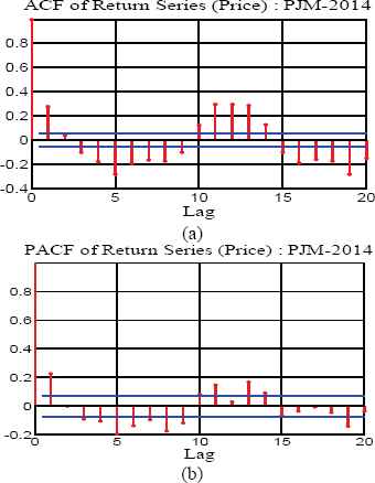
ACF and PACF plots for the 2014 PJM Return Price Data
The proposed methodology for predicting electricity price time series is implemented using PJM electricity market data from January 1, 2014 to December 31, 2014. In all the considered weeks of forecast, for a particular day’s forecast, the training dataset is used for the prior 20 days. The inputs to all the proposed models comprise the return price time series given by the lags of (t-23), (t-24), (t-47), (t-48), (t-71), (t-72), (t-95), and (t-96) hours, respectively. The training data comprises the actual price data up to the day before the day of forecast. Keeping in view of seasonal variations, four different periods have been chosen to evaluate the performance of the proposed models. The four one-week periods include February 1-7, May 1-7, August 1-7, and November 1-7 of the year 2014. Originally the electricity data set has been divided into training and testing sets.
As the evolutionary algorithms are based on randomness, the performance metrics are observed from ten independent executions of the algorithm with same training and testing sets. The stability of prediction is ascertained from the convergence characteristics shown in Fig.5 for both the FF and IFFHS algorithms. The LRNFIS trained by conventional FF algorithm takes nearly 60 iterations to converge, whereas the IFFHS algorithm takes nearly 40 iterations with less error in the objective function. Table-1 provides the details of the various settings of the hybrid IFFHS algorithm.

Convergence characteristics of the FF and IFFHS algorithms
| Parameters | Values |
|---|---|
| Maximum number of generation (Tmax) | 100 |
| Total number of fireflies (Nff) | 20 |
| Initial randomization parameter (γ) | 0.5 |
| Absorption co-efficient (β) | 0.8 |
| Maximum and minimum attractiveness (βmax and βmin) | 0.95 & 0.3 |
| Maximum and minimum PAR (PARmax & PARmin) | 0.9 & 0.3 |
| Maximum and minimum bw (BWmax & BWmin) | 0.5 & 0.2 |
| Harmonic consideration rate (HMCR) | 0.8 |
Details of proposed IFFHS algorithm
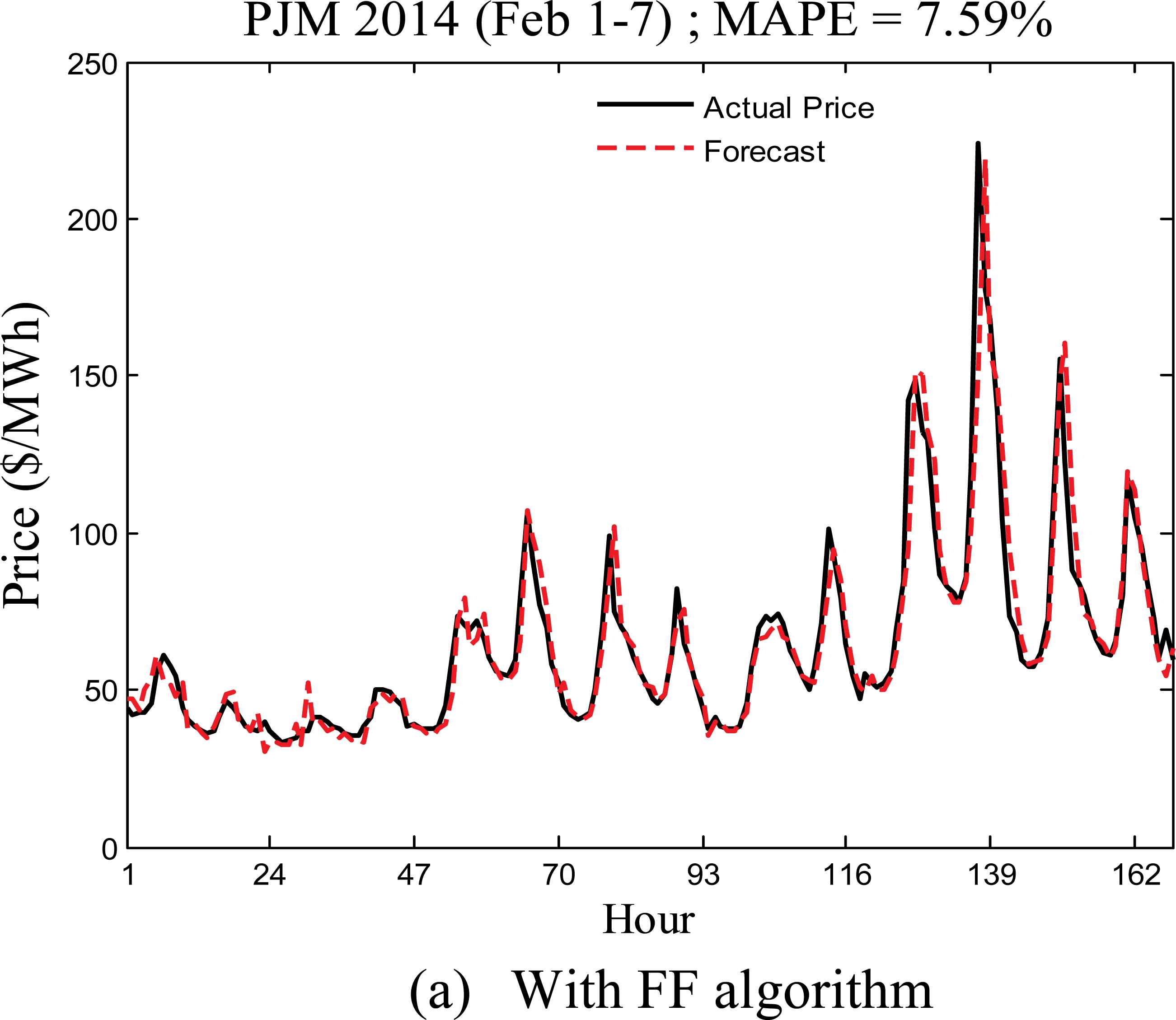
Figs. 6(a) to 6(h) show the weekly forecasts for the first weeks of February, May, August, and November, respectively using both the FF and IFFHS algorithm, and the MAPE values are also given in Table-2. From the results it is clearly seen that the actual values of electricity prices in the considered week of November, 2014 are captured more accurately in comparison to the weekly forecast during Feb.1-7, 2014. This discrepancy indicates the presence of low spikes in electricity prices in November as compared to those in the month of February 2014. The MAPE is found to be 6.30 % during Nov.1-7 using FF based LRNFIS in comparison to 5.27% for the IFFHS based LRNFIS. Similarly the period of August 1-7 exhibits MAPE value of 4.23% for the FF-LRNFIS compared to 4.02% for the IFFHS-LRNFIS. Table-2 provides the weekly comparison of MAPE values for different typical months of the year. Further a comparison with the well known radial basis function neural network (RBFNN) and functional link neural network using IFFHS algorithm for weight parameter training is given in Table-2, showing clearly the superiority of prediction performance of the LRNFIS with IFFHS algorithm over RBFNN and FLANN models.
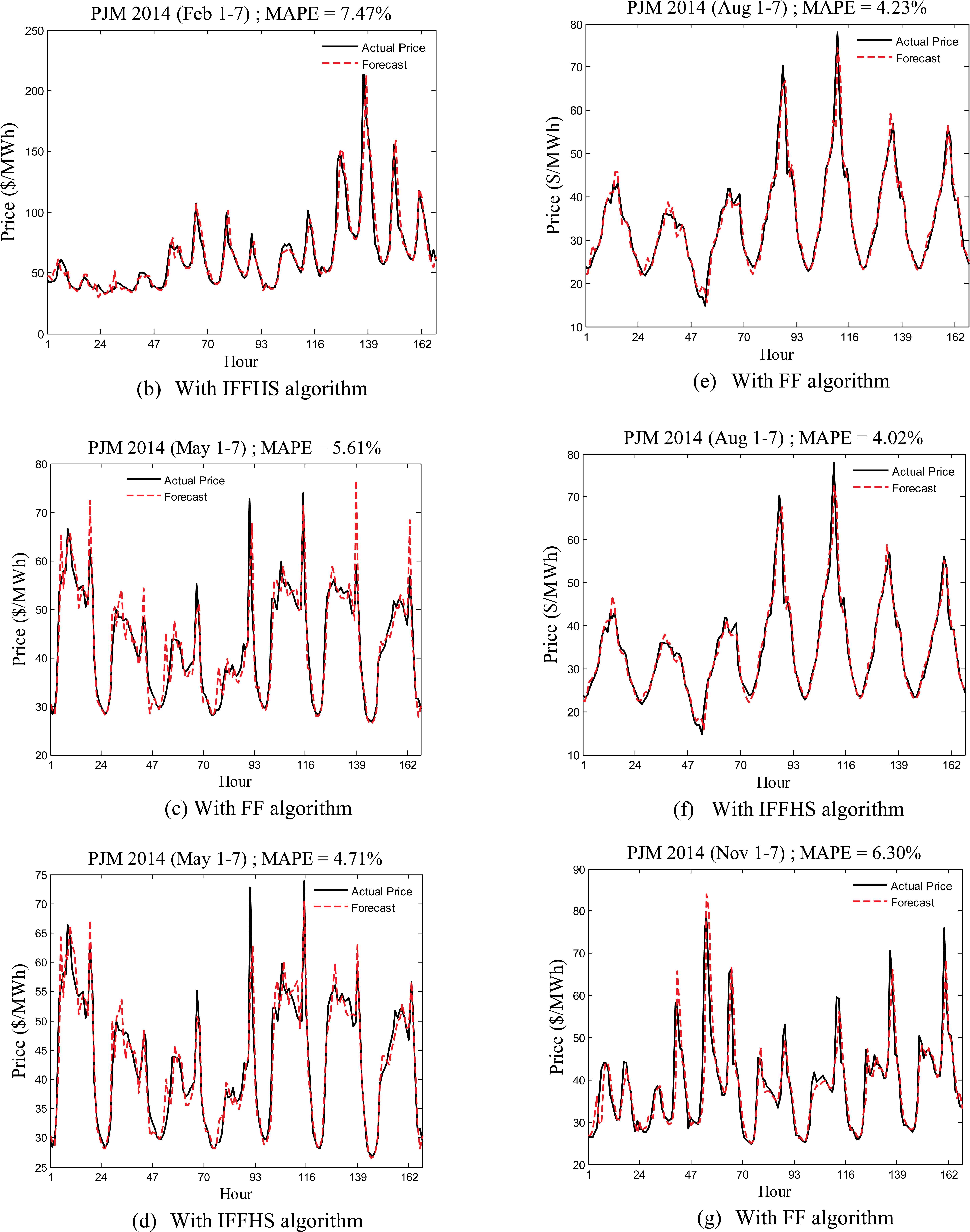
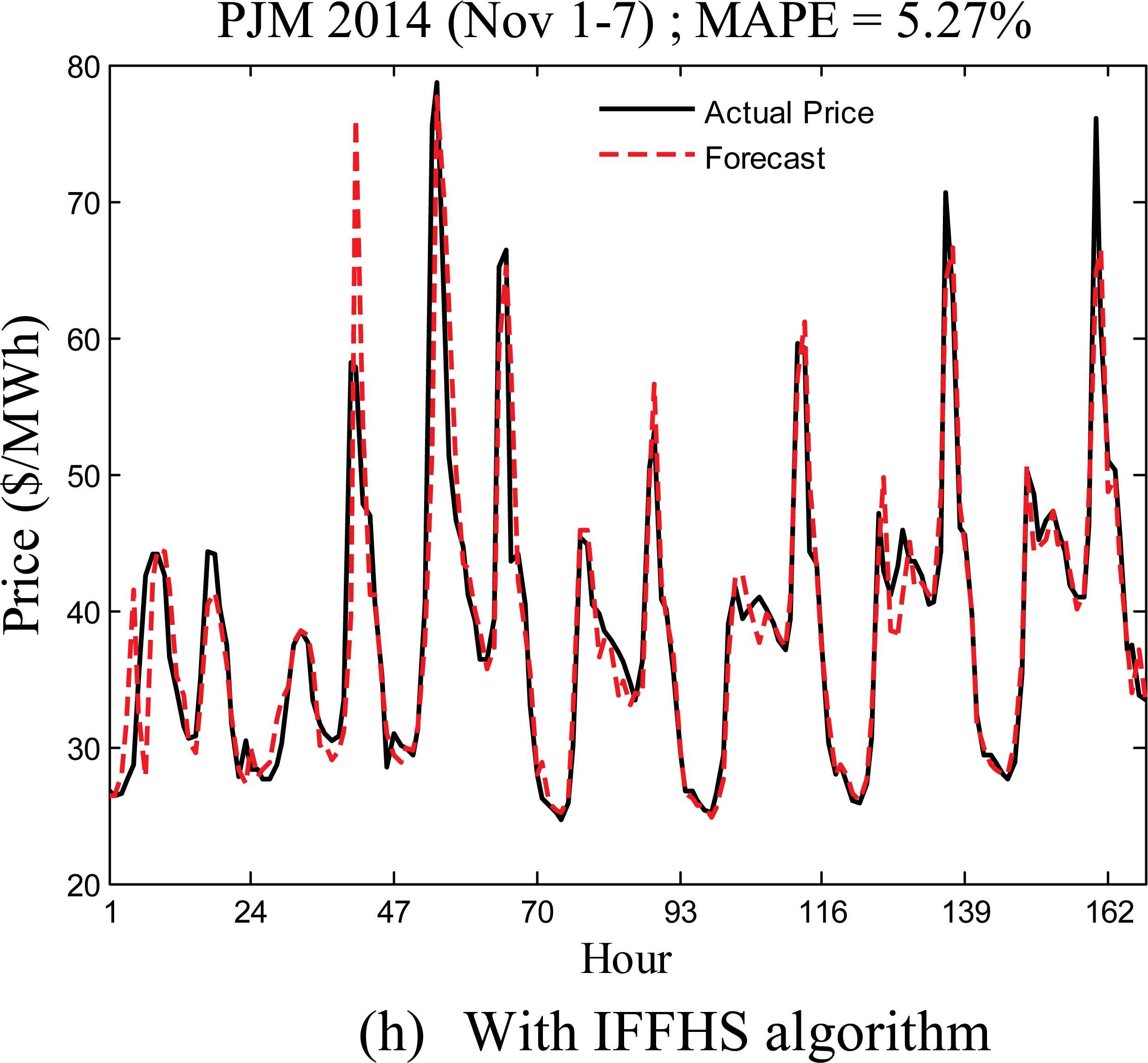
Seasonal MAPE variations for the PJM Electricity market during the year 2014 using LRNFIS
| Period | LRNFIS with FF | LRNFIS with IFFHS | RBFNN with IFFHS | FLANN with IFFHS | ||||
|---|---|---|---|---|---|---|---|---|
| RMSE | MAPE | RMSE | MAPE | RMSE | MAPE | RMSE | MAPE | |
| Feb 1-7 | 0.0093 | 7.59 | 0.007 | 7.47 | 0.0098 | 8.73 | 0.016 | 9.26 |
| May 1-7 | 0.0056 | 4.94 | 0.0041 | 4.71 | 0.0074 | 5.83 | 0.0097 | 6.13 |
| Aug 1-7 | 0.0047 | 4.23 | 0.0040 | 4.02 | 0.0062 | 5.76 | 0.0089 | 6.06 |
| Nov 1-7 | 0.0072 | 6.30 | 0.0053 | 5.27 | 0.0084 | 7.35 | 0.012 | 7.95 |
RMSE and MAPE (%) of PJM Electricity market
The three models namely the LRNFIS with FF, LRNFIS with IFFHS, and RBFNN with IFFHS algorithm are subjected to Superior ability performance test to provide a comparison of their relative performance except the FLANN, which gives the worst performance. To avoid the data snooping problem, the upper and lower bound of the SPA test over MAPE errors have been calculated for the PJM weekly electricity market data used for prediction as shown in Table-3. Table-3 presents the P-values of upper and lower bound of SPA test with 3 different size of bootstrap re-samples namely 500, 800, and 1000 chosen from the 2014 year. In this test each model is considered individually as the benchmark model to evaluate whether a particular model is significantly outperformed by other competing models. For the considered data sets, the P-value of SPA test over MAPE error with different bootstrap size is showing higher value indicating that the other competing models are not producing better performance compared to the proposed model. From Table-3 it is clearly observed that the LRNFIS model with IFFHS model completely outperforms the LRNFIS model with FF and RBFNN model trained by IFFHS algorithms in predicting the electricity price time series.
| Benchmark model | No. of Bootstraps |
|||||
|---|---|---|---|---|---|---|
| 500 | 800 | 1000 | ||||
| SPAu | SPAl | SPAu | SPAl | SPAu | SPAl | |
| LRNFIS with IFFHS | 0.984 | 0.760 | 0.969 | 0.678 | 0.975 | 0.547 |
| LRNFIS with FF | 0.835 | 0.692 | 0.817 | 0.562 | 0.834 | 0.532 |
| RBFNN with IFFHS | 0.717 | 0.583 | 0.754 | 0.435 | 0.713 | 0.482 |
P-value of Superior Predictive Ability test over MAPE error for PJM Electricity market
Dataset-2:
After establishing the superior performance of the LRNFIS model trained by the IFFHS evolutionary algorithm in electricity price time series prediction, its performance is evaluated for one day ahead prediction of daily currency exchange rates for datset-2. Four major currencies such as Australian Dollar (AUD), Swiss Francs (CHF), Mexican Pesos (MXN), and Brazilian Dollar (BRL) against US Dollar (USD) are chosen for experimental analysis. Each currency exchange dataset covers time span from January 2010 to March 2013 and contains 800 data out of which initial 500 data are taken for training and the following 300 data are taken for testing. The details are depicted in Table-4. Before starting the training process, the data (actual prices) are normalized between 0 and 1 using the min-max formula using eq.(42). In this case five lagged scaled prices are used as inputs for current day price prediction i.e. the price on current day ‘d’ depends on the prices of days ‘d-1’, ‘d-2’, ‘d-3’, ‘d-4’, ‘d-5’ and this concept is followed for each day ahead price prediction for the training and testing datasets. Once the training process of the LRNFIS model completes then the testing is started with the optimized weights from the training.
- y
= normalized value.
- pr
= value to be normalized
- prmin
= minimum value of the series to be normalized
- prmax
= maximum value of the series to be normalized
| Datasets-2 | Currency Exchange rates against US Dollar | Training Period | Testing Period |
| AUD/USD | January | January | |
| CHF/USD | 2010 to | 2012 to | |
| MXN/USD | December | March | |
| BRL/USD | 2011 | 2013 | |
Datasets chosen for experimental study
The testing performances of the currency exchange rates prediction are measured in terms of MAPE, MSE, RMSE and are shown in Table-5. From Table-5 it is clear that the four currency exchange rates prediction show an average MAPE of 0.5 and the MSE and RMSE are very small. The one-day ahead testing results (Target vs Predicted) of AUD/USD, CHF/USD, MXN/USD, BRL/USD are depicted in Figs. 7, 8, 9, and 10, respectively.

AUD/USD predicted Testing results

CHF/USD predicted Testing results
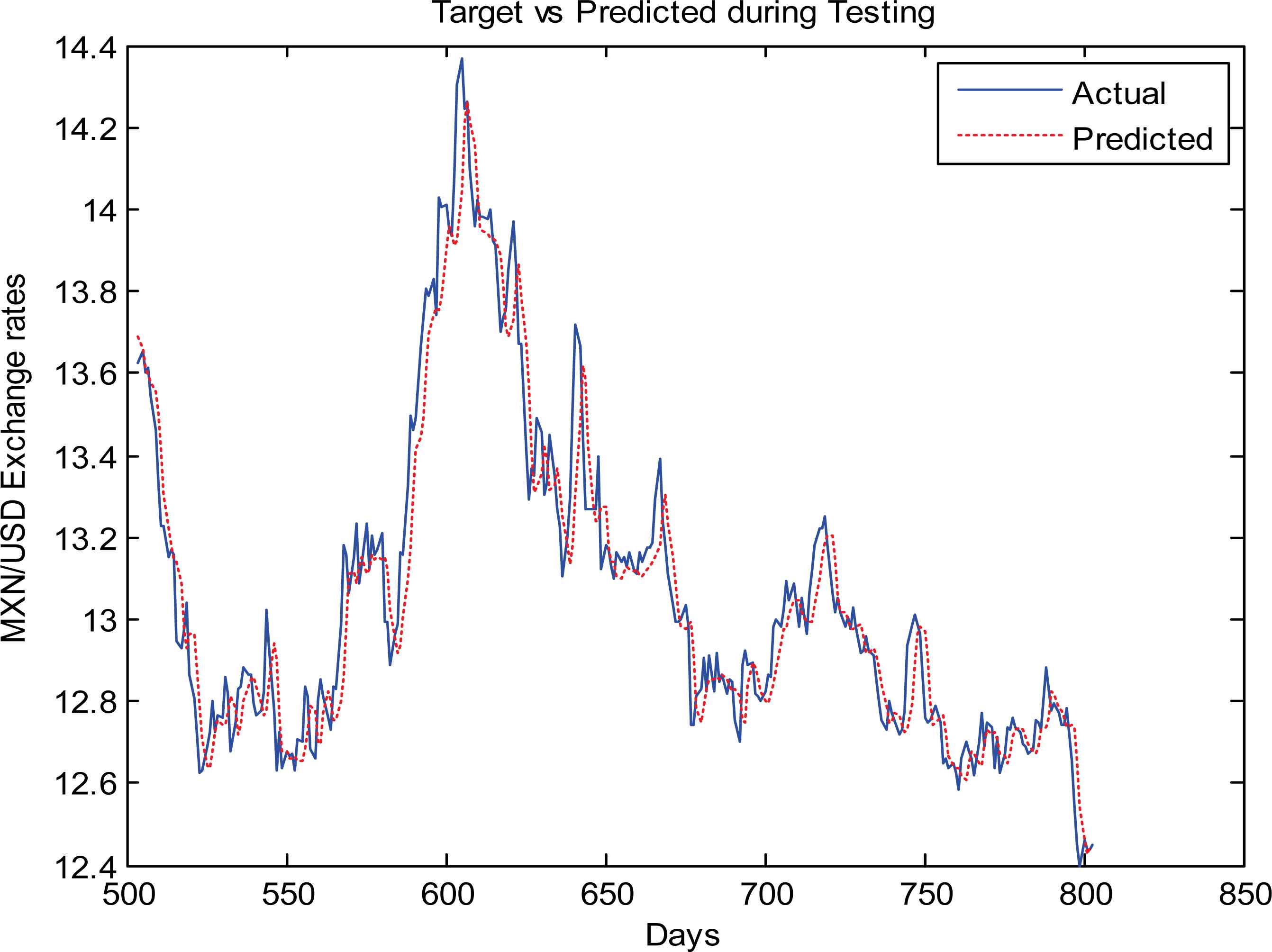
MXN/USD predicted Testing results

BRL/USD predicted Testing results
| 1-day ahead prediction |
|||
|---|---|---|---|
| Currency Exchange rates against US Dollar | MAPE | MSE | RMSE |
| AUD/USD | 0.5391 | 4.2665e-05 | 0.0065 |
| CHF/USD | 0.5724 | 4.5064e-05 | 0.0067 |
| MXN/USD | 0.5692 | 0.0100 | 0.1001 |
| BRL/USD | 0.5872 | 2.5305e-04 | 0.0159 |
| 5-days ahead prediction | |||
| AUD/USD | 0.7305 | 7.9477e-05 | 0.0089 |
| CHF/USD | 0.8419 | 8.8983e-05 | 0.0094 |
| MXN/USD | 0.6234 | 0.0127 | 0.1125 |
| BRL/USD | 0.8441 | 4.9434e-04 | 0.0222 |
| 7-days ahead prediction | |||
| AUD/USD | 0.8816 | 1.0355e-04 | 0.0102 |
| CHF/USD | 0.9026 | 1.1235e-04 | 0.0106 |
| MXN/USD | 0.9123 | 0.0249 | 0.1578 |
| BRL/USD | 0.9044 | 7.1107e-04 | 0.0267 |
| 10-days ahead prediction | |||
| AUD/USD | 1.0188 | 1.4035e-04 | 0.0118 |
| CHF/USD | 1.1884 | 1.6995e-04 | 0.0130 |
| MXN/USD | 1.2098 | 0.0417 | 0.2042 |
| BRL/USD | 1.1218 | 9.7488e-04 | 0.0312 |
Performance Evaluation using Datasets 2
The model has again been verified by predicting the 5-days, 7-days, and 10-days ahead currency exchange rates and findings from these experiments are given in Table-5 and graphical prediction results are shown in Figs. 11–14. Fig.11 shows the 5-days, 7-days, and 10-days ahead prediction of AUD/USD where as Fig.12 depicts the 5-days, 7-days, and 10-days ahead prediction of CHF/USD, respectively. Similarly the MXN/USD and BRL/USD prediction results are shown in Figs.13 and 14, respectively.
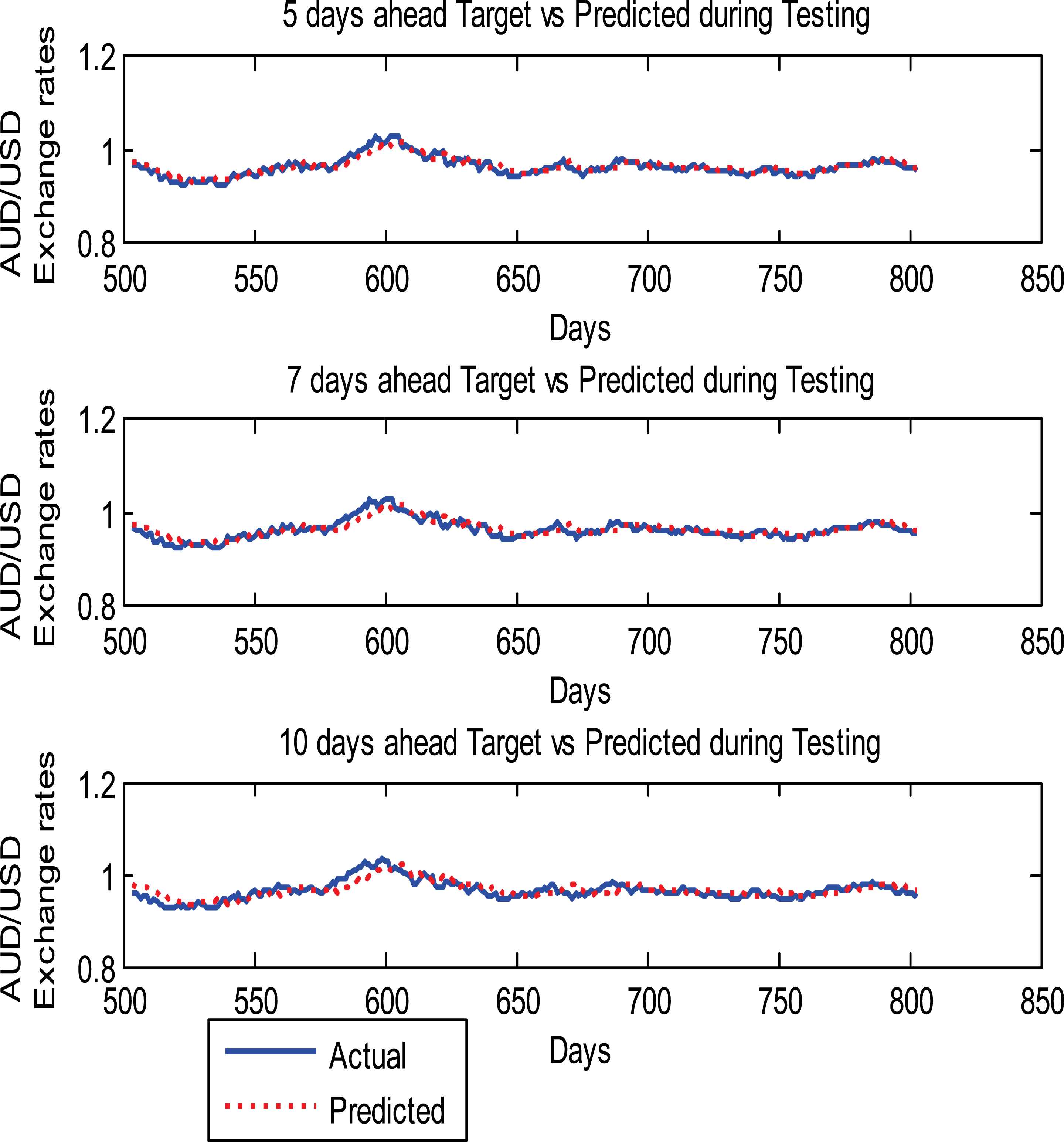
5, 7, and 10 -days ahead prediction results of AUD/USD Currency exchange rates

5, 7, and 10 -days ahead prediction results of CHF/USD Currency exchange rates

5,7 and 10 -days ahead prediction results of MXN/USD Currency exchange rates
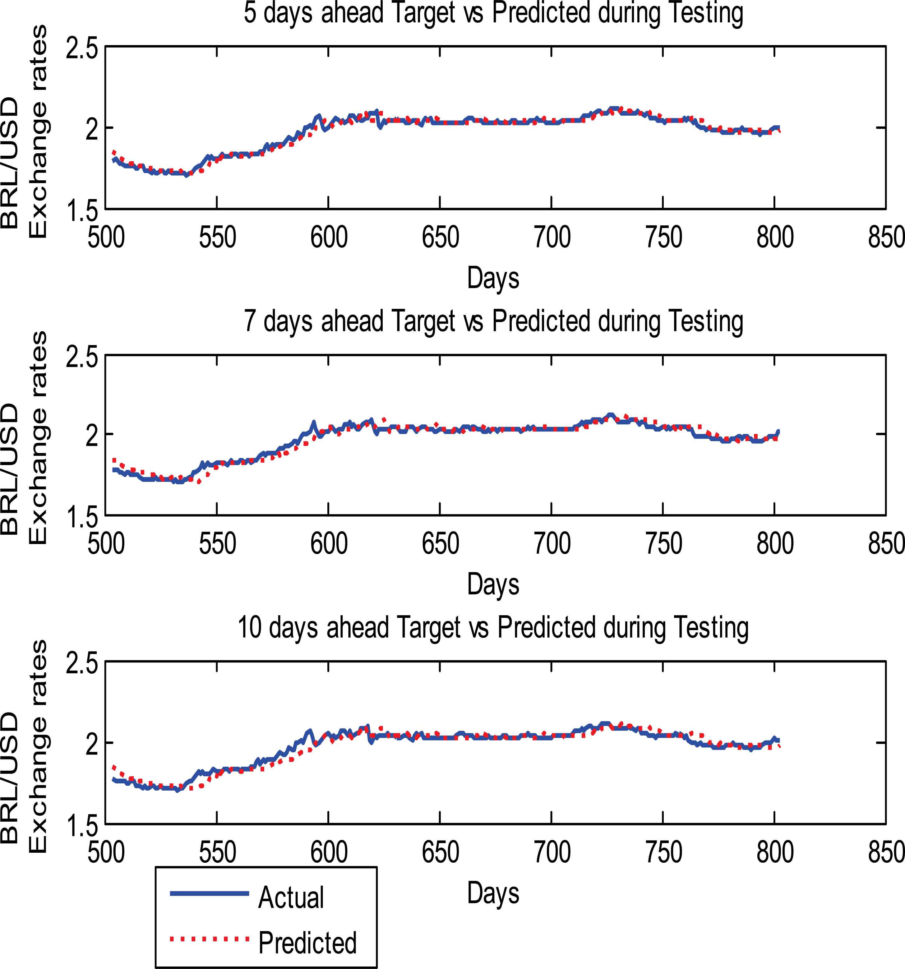
5,7 and 10 -days ahead prediction results of BRL/USD Currency exchange rates
From Table-5, it is clear that the average MAPE for the four chosen currency exchange rates for one day ahead prediction is 0.5. The 5-days, 7-days, and 10-days ahead predictions MAPE of AUD/USD are 0.7305, 0.8816, and 1.0188, respectively. The 10-days ahead prediction MAPE is higher than 5-days and 7-days ahead prediction MAPE. The MAPEs for AUD/USD prediction result are lower as compared to the CHF/USD, MXN/USD, and BRL/USD which indicates that the AUD/USD prediction performance is better than the other three currency exchange rates.
Dataset-3:
The LRNFIS model further proves its efficiency using two other stock market time series datasets: Standard & Poor’s 500 stock market abbreviated as S&P 500, an American stock market and Nikkei 225 commonly known as Nikkei Index from Tokyo stock exchange. The daily closing prices of S&P 500 and Nikkei 225 stock market are collected for the purpose of day ahead price prediction. Each of the two considered datasets contains 800 data covering the time span from 04 January 2010 to 04 March 2013 out of which the first 500 data from 04 January 2010 to 23 December 2011 are chosen for training the model and the rest 300 data from 27 December 2011 to 04 March 2013 are taken for testing to prove the efficiency of the model. Here the data processing is similar to the procedure used for Dataset-2. The testing outcomes of the two stock markets are presented in Table-6 and the graphical representation of the testing results shown in Figs. 15 and 16 which validate the performance of the testing results. The S&P 500 testing performance shows a MAPE of 0.6288 and Nikkei 225 shows a MAPE of 0.7105 which proves the efficiency of the LRNFIS model.

S&P 500 Testing Results

Nikkei 225 Testing Results
| 1-day ahead prediction | |||
|---|---|---|---|
| Stock market | MAPE | MSE | RMSE |
| S&P 500 | 0.6288 | 2.5745e-04 | 0.0160 |
| Nikkei 225 | 0.7105 | 2.6089e-05 | 0.0051 |
Performance Evaluation using Datasets 3
6. Conclusion
A new locally recurrent neuro-fuzzy information system (LRNFIS) is presented in this paper for time series prediction. The LRNFIS uses TSK type fuzzy rule base where the consequent part comprises Chebyshev polynomial functions providing an expanded nonlinear transformation of the inputs suitable for forecasting chaotic time series. Further dynamic memory is provided by using locally recurrent nodes after the fuzzy output normalization layer allowing past and present inputs to be used for a robust prediction. The weights of the LRNFIS are trained by an improved firefly harmony search algorithm whereas the membership functions of the fuzzy system are learnt by a gradient descent algorithm. The performance of the proposed LRNFIS is validated by using three real world time series data sets namely the PJM electricity market, currency exchange market (AUD/USD, CHF/USD, MXN/USD, BRL/USD), and S&P 500 and Nikkei 225 stock markets providing robust prediction results. A comparison with widely used RBFNN is presented, which also reveals the same conclusion. Further a superior predictive ability test is used to choose the correct forecasting model.
References
Cite this article
TY  - JOUR
AU  - A.K. Parida
AU  - R. Bisoi
AU  - P.K. Dash
AU  - S. Mishra
PY  - 2017
DA  - 2017/01/01
TI  - Times Series Forecasting using Chebyshev Functions based Locally Recurrent neuro-Fuzzy Information System
JO  - International Journal of Computational Intelligence Systems
SP  - 375
EP  - 393
VL  - 10
IS  - 1
SN  - 1875-6883
UR  - https://doi.org/10.2991/ijcis.2017.10.1.26
DO  - 10.2991/ijcis.2017.10.1.26
ID  - Parida2017
ER  -