
A New Criterion for Soft Set Based Decision Making Problems under Incomplete Information
- DOI
- 10.2991/ijcis.2017.10.1.27How to use a DOI?
- Keywords
- Soft set; Incomplete soft set; Choice value; Decision making
- Abstract
We put forward a completely redesigned approach to soft set based decision making problems under incomplete information. An algorithmic solution is proposed and compared with previous approaches in the literature. The computational performance of our algorithm is critically analyzed by an experimental study.
- Copyright
- © 2017, the Authors. Published by Atlantis Press.
- Open Access
- This is an open access article under the CC BY-NC license (http://creativecommons.org/licences/by-nc/4.0/).
1. Introduction
In this paper we revisit the soft set based decision making problem under incomplete information as approached by Han et al. 14, Qin et al. 21, and Zou and Xiao 36.
Many real life problems require the use of imprecise or uncertain data (cf., Kahraman et al. 15). Their analysis must involve the application of mathematical principles capable of capturing these features. Fuzzy set theory meant a paradigmatic change in mathematics which allows partial membership. The publication of Zadeh’s seminal article 31 has triggered a vast literature on fuzzy sets and their applications, which includes a number of successful generalizations.
Of these variations we are especially interested in the application of soft sets theory and their extensions to decision making problems (cf., Molodtsov 20 for a definition and arguments about its applicability to several fields). Further relevant references include Aktaş and Çağman 1, Alcantud 3, Ali 5,6, Ali et al. 7, and Maji et al. 19. Ali et al. 8 define lattice ordered soft sets for situations where some order exists among the elements of the parameter set. Qin et al. 23 combine interval sets and soft sets, and Zhang 35 studies interval soft sets. Maji, Biswas and Roy 17 introduce fuzzy soft sets (see also Ali and Shabir 9 for techniques that permit to study logic connectives for soft sets and fuzzy soft sets, and Alcantud 2 for a recent decision-making procedure based on fuzzy soft sets). Relatedly, Shao and Qin 27 define fuzzy soft lattices and discuss their structure. Wang, Li and Chen 29 introduce hesitant fuzzy soft sets. As mentioned above, Han et al. 14, Qin et al. 21, and Zou and Xiao 36 are concerned with incomplete soft sets. Rodríguez et al. 24,25 are recent surveys on hesitant fuzzy sets (cf., Torra 28). There are also interesting hybrid models in recent literature, e.g., rough soft hemirings (a new rough set theory which is an extended notion of a rough hemiring and a soft hemiring) in Zhan et al. 32,33, or Z-soft rough fuzzy ideals of hemirings (cf., Zhan and Zhu 34).
Maji, Biswas, and Roy 18 pioneered soft set based decision making. They established the criterion that an object can be selected if it maximizes the choice value of the problem. Relatedly, Zou and Xiao 36 argued that in the process of collecting data there may be unknown, missing or inexistent data. Therefore, standard soft sets under incomplete information must be taken into account, which calls for the inspection of incomplete soft sets. Afterwards Han et al. 14 and even Qin et al. 21 present other interesting approaches to incomplete soft set based decision making. However, in the frequent cases in which there is perfect uncertainty about the real value of the missing data, it seems appropriate to proceed with a decision making procedure that avoids estimations. This is the purpose of the present contribution.
Our paper contributes to decision making studies in the context of incomplete soft sets from an altogether different perspective. We propose to go through all the filled tables that can be produced from the original incomplete table. All cases are evaluated according to their respective choice values, and finally the alternatives are ranked by the proportion of tables in which they receive the highest choice value.
Our proposal is justified by a classical Laplacian argument from probability theory. Under Laplace’s principle of indifference, due to our complete ignorance we are entitled to assume that all tables in which the *’s can be replaced with either 0 or 1 are equiprobable. It is sensible to compute the objects which should be selected according to soft-set based decision making in each of these cases in order to make a decision for any object that is selected in the highest proportion of cases.
The use of probabilities in decision making under incomplete information in soft sets already appears in Zou and Xiao’s 36 seminal article as a tool that permits to attach weights to the possible choice values of the options. Nevertheless, we provide examples which prove that our solution is indeed different from theirs and other proposed approaches in the existing literature. Consequently, pretty simple situations confirm that making decisions according to our methodology produces decisions that do not necessarily coincide with solutions in the literature. We discuss some issues of efficiency of our Algorithm by means of a computational experiment.
This paper is organized as follows: Section 2 retrieves some terminology and definitions. We define a notion of domination of alternatives that is used in our decision making algorithm. Section 3 contains a review of the solutions proposed by earlier investigations as well as our proposal and an illustrative example. Then we compare our algorithm with previous solutions in order to ensure its novelty. In subsection 3.5 the computational features of our proposal are examined, too. Finally, our conclusions are in Section 4.
2. Definitions: Soft Sets and Incomplete Soft Sets
We adopt the usual description and terminology for soft sets and their extensions: U denotes a universe of objects and E denotes a universal set of parameters.
Definition 1.
[Molodtsov 20] A pair (F,A) is a soft set over U when A ⊆ E and F : A → 𝒫(U), where 𝒫(U) denotes the set of all subsets of U.
A soft set over U is regarded as a parameterized family of subsets of the universe U, the set A being the parameters. For each parameter e ∈ A, F(e) is the subset of U approximated by e or the set of e-approximate elements of the soft set. Many scholars have performed formal investigations of this and related concepts. For example, Maji, Bismas and Roy 19 develop this notion and define among other concepts: soft subsets and supersets, soft equalities, intersections and unions of soft sets, et cetera. Furthermore, Feng and Li 12 give a systematic study on several types of soft subsets and various soft equal relations induced by them. Concerning (pure) soft set based decision making, we refer the reader to Çağman and Enginoğlu 10, Maji, Biswas and Roy 18, and Feng et al. 13
In order to model increasingly general situations, Definition 2 below has been subsequently proposed and investigated:
Definition 2.
[Han et al. 14] A pair (F,A) is an incomplete soft set over U when A ⊆ E and F : A → {0,1,∗}U, where {0,1,∗}U is the set of all functions from U to {0,1,∗}.
Obviously, every soft set can be considered an incomplete soft set. The ∗ symbol in Definition 2 permits to capture “lack of information”: when F(e)(u) = ∗ we interpret that u belongs to the subset of U approximated by e is unknown. As in the case of soft sets, when F(e)(u) = 1 (resp., F(e)(u) = 0), we interpret that u belongs (resp., does not belong) to the subset of U approximated by e.
As is well known since the early antecedent in Yao 30, when both U and A are finite (as in the application references mentioned above), soft sets and incomplete soft sets can be represented either by matrices or in tabular form. Rows are attached with objects in U, and columns are attached with parameters in A. In the case of a soft set, these representations are binary (i.e., all cells are either 0 or 1).
3. The Problem: Preliminaries and New Proposals of Solution
In this section we tackle the problem of applying incomplete soft sets in decision making practice.
3.1. Preliminaries and Antecedents
Concerning (pure) soft set based decision making, the fundamental reference is Maji, Biswas and Roy 18. When a soft set (F,A) is represented in matrix form through the matrix (ti j)k × l, where k and l are the cardinals of U and A respectively, then the choice value of an object hi ∈ U is ci = ∑j ti j. A suitable choice is made when the selected object hk verifies ck = maxi ci. In other words, objects that maximize the choice value are satisfactory outcomes of this decision making problem.
Concerning incomplete soft set based decision making, the most successful approaches are probably Han et al. 14, Qin et al. 21, and Zou and Xiao 36. Let us survey their ideas.
Zou and Xiao 36 initiated the analysis of soft sets and fuzzy soft sets under incomplete information. In the first, standard case they propose to calculate all possible choice values for each object, and then calculate their respective “decision values” di by the method of weighted-average. To this purpose the weight of each possible choice value is computed by existing complete information. In particular, they put forward some simple indicators that can eventually be used to prioritize the alternatives, namely, ci(0) (the choice value if all missing data are assumed to be 0), ci(1) (the choice value if all missing data are assumed to be 1) and di−p (which is easily shown to correspond to (ci(0) + ci(1))/2).
Because Zou and Xiao’s definition of di is complex and difficult to understand, Kong et al. 16 have designed a simplified approach to decision making for incomplete soft sets that is equivalent to the weight-average of all possible choice value approach.
Inspired by the data analysis approach in Zou and Xiao 36, Qin et al. 21 propose a new way to fill out the missing data in an incomplete soft set. To that purpose, they introduce the relation between parameters. Thus, they prioritize the association between parameters rather than the probability of objects appearing in F(ei). This way they attach a completed soft set with any incomplete soft set. However, the procedure of Qin et al. 21 presupposes that there are associations among some of the parameters. Their proposal relies on to Zou and Xiao’s method 36: when an exogenously given threshold is not reached, the data is filled out according to Zou and Xiao’s approach. Incidentally, there is no clue as to which threshold is suitable for each problem.
Qin et al. hint that their procedure can be used to implement subsequent applications involving incomplete soft sets, but they do not make any explicit statement as to decision making. In fact, these authors criticize the approach for (crisp) soft sets in Zou and Xiao 36 because the missing data are still missing at the end of the process, and “the soft sets cannot be used in other fields but decision making”. Nevertheless, it seems appropriate to complement their filling procedure with a prioritization of the objects according to their choice values Qi, as is standard in soft-set based decision making. Han et al. 14, section 1.3, explain that “this method is good when objects in U are related with each other”.
Relatedly, we also mention that Khan et al. 26 deal with predicting the performance of handling missing data in incomplete soft sets, but they do not advocate for any decision making mechanism. Therefore Khan et al. 26, like Qin et al. 21, are not directly concerned with decision making mechanisms.
Finally, Han et al. 14 develop and compare several elicitation criterions for decision making of incomplete soft sets which are generated by restricted intersection. Here we do not pursue that avenue.
Table 1 summarizes the definitions of elements that we have explained above.
| Index | Description | Source |
|---|---|---|
| di | Calculate all possible choice values for each object. Then calculate their di by method of weighted-average |
Zou & Xiao 36 Kong et al. 16 |
| di−p | (ci(0) + ci(1))/2 | Zou & Xiao 36 |
| ci(0) | Choice value if missing data are 0 | Zou & Xiao 36 |
| ci(1) | Choice value if missing data are 1 | Zou & Xiao 36 |
| Qi | Choice value of soft set completed by data filling approach | Own ellaboration from Qin et al. 21 |
Indicators that permit to make decisions about soft sets in an environment with incomplete information.
3.2. A Preparatory Step
Here we comment upon some solutions in Zou and Xiao 36. Let us fix an incomplete soft set.
The researcher can conduct a pre-screening operation before selecting a final option. We calculate the maximum value c0 of all choice values cj(0) across options uj. If this value is strictly greater than the choice value ck(1) of an alternative uk, this alternative can be removed from the initial matrix. The reason is that if all missing data for uk are assumed to be 1, there is another option i verifying that when all missing data for ui are assumed to be 0, still option i has a greater choice value than option k. This argument suggests the following novel definition:
Definition 3.
Let (F,A) be an incomplete soft set over U. An option i dominates an option k when ck(1) < ci(0).
Clearly, if we adhere to any choice value based solution, we can freely discard dominated options. For example, if we use either dj, cj(0), cj(1) or dj−p as an indicator for any option j, option k cannot maximize the selected indicator when option i dominates it.
This simplification is basically inconsequential in the case of Zou and Xiao’s solutions, however we can apply it in other computationally costly algorithms in order to reduce calculations.
3.3. A New Proposal of Solution
We must emphasize that our purpose here is not to fill any missing data but to give advice on which choice should be made when data are missing in the context of soft sets. Due to the criticisms raised above, to that purpose we cannot support the idea that averages, probabilities or any other specific evaluations should be used to fill missing data. Given that generally there is perfect uncertainty about the real value of these absent data, we propose a completely different approach. We evaluate each feasible filled table according to their choice value. Then we order the alternatives by the proportion of tables where they receive the highest choice value.
The intuition for our proposal is as follows. According to Laplace’s principle of indifference in probability theory, under complete ignorance we must assume that all tables where the ∗’s are replaced with either 0 or 1 are equiprobable. Hence the best we can do is to compute which objects should be selected according to soft-set based decision making in each of these cases, and then opt for any object that is optimal in the highest proportion of cases with completed information.
In accordance with this idea and our arguments in section 3.2, we endorse the following algorithm for the problems where both U and A are finite:
|
Incomplete Soft Sets Algorithm
Observe that because choice values can be repeated at each Cv matrix, one has
We can reinterpret the Algorithm above as follows. Firstly, we eliminate dominated alternatives at Step 2. Suppose that due to our complete ignorance of the real data, all completed soft sets from the input of the problem are considered equally probable. Suppose that in case of (complete) soft set problems, we opt for any object with the highest choice value. Then a solution for our original problem is any object such that the probability of its being a solution of a randomly selected completed soft set problem (that is to say, si = ni/2w) is maximal.
The following example from real practice illustrates our proposal. Afterwards we use it to explain the fundamentals of our proposal in practical terms.
Example 1.
Let U = {h1,h2,h3} be a universe of houses. With respect to the set of parameters (or attributes or house characteristics) E0 = {e1,e2,e3,e4} the following information is known in the form of an incomplete soft set (F0,E0):
- (a)
h1 ∈ F0(e1) ∩ F0(e3) and h1 ∉ F0(e4), but it is unknown whether h1 ∈ F0(e2) or not.
- (b)
h2 ∈ F0(e2) and h2 ∉ F0(e3) ∪ F0(e4), but it is unknown whether h2 ∈ F0(e1) or not.
- (c)
h3 ∈ F0(e1) ∩ F0(e4) and h3 ∉ F0(e2) ∪ F0(e3).
- (d)
h4 ∉ F0(e1) ∪ F0(e2) ∪ F0(e4), but it is unknown whether h4 ∈ F0(e3) or not.
Table 2 captures the information defining (F0,E0). We observe that houses 1 and 3 dominate house 4, hence h4 is eliminated and a 3 × 4 table remains. In such trimmed table we have w = 2, and we enumerate the cells with value ∗ as ((1,2), (2,1)).
| e1 | e2 | e3 | e4 | |
|---|---|---|---|---|
| h1 | 1 | ∗ | 1 | 0 |
| h2 | ∗ | 1 | 0 | 0 |
| h3 | 1 | 0 | 0 | 1 |
| h4 | 0 | 0 | ∗ | 0 |
Tabular representation of the incomplete soft set (F0,E0) in Example 1.
For each v ∈ {0,1}w = {v1 = (0,0), v2 = (0,1), v3 = (1,0), v4 = (1,1)} one feasible completed table arises. These four tables are represented in Table 3, together with the choice values of the houses at each table. We observe that h1 attaches the highest choice value at all these four tables, h2 attaches the highest choice value at Cv2 only, and h3 attaches the highest choice value exactly at Cv1 and Cv2. Therefore we easily obtain the s1,s2,s3 scores as in Step 5.
| Cv1 matrix |
Cv2 matrix |
||||||||||
| e1 | e2 | e3 | e4 | ci | e1 | e2 | e3 | e4 | ci | ||
| h1 | 1 | 0 | 1 | 0 | 2 | h1 | 1 | 0 | 1 | 0 | 2 |
| h2 | 0 | 1 | 0 | 0 | 1 | h2 | 1 | 1 | 0 | 0 | 2 |
| h3 | 1 | 0 | 0 | 1 | 2 | h3 | 1 | 0 | 0 | 1 | 2 |
| Cv3 matrix |
Cv4 matrix |
||||||||||
| e1 | e2 | e3 | e4 | ci | e1 | e2 | e3 | e4 | ci | ||
| h1 | 1 | 1 | 1 | 0 | 3 | h1 | 1 | 1 | 1 | 0 | 3 |
| h2 | 0 | 1 | 0 | 0 | 1 | h2 | 1 | 1 | 0 | 0 | 2 |
| h3 | 1 | 0 | 0 | 1 | 2 | h3 | 1 | 0 | 0 | 1 | 2 |
The four completed tables for the incomplete soft set (F0,E0) according to Step 4 in our Algorithm, with the respective choice values for each alternative.
Table 4 contains this information as well as the indicators by other focal proposals of solution for this problem, as defined in section 3.1. The optimal alternatives for each procedure are represented too. In addition, observe that the fact that houses 1 and 3 dominate house 4 stems from Table 4 by comparing the maximum of column ci(0) —which is attained at 1 and 3— and the values in column ci(1) that are strictly smaller than such maximum.
| si | di | di−p | ci(0) | ci(1) | Qi | |
|---|---|---|---|---|---|---|
| h1 | 1.00 | 2.50 | 2.50 | 2 | 3 | 3 |
| h2 | 0.25 | 2.00 | 1.50 | 1 | 2 | 1 |
| h3 | 0.50 | 2.00 | 2.00 | 2 | 2 | 2 |
| h4 | 0 | 0.33 | 0.5 | 0 | 1 | 1 |
| Optimal | {h1} | {h1} | {h1} | {h1,h3} | {h1} | {h1} |
Solutions for the problem represented by (F0,E0) in Example 1 according to various indicators (v., Algorithm 1 and Table 1).
In order to explain how the intuition of our idea applies to this example, we take advantage of the very competent introduction to incomplete soft sets in real practice by Han et al. 14. Maybe the indeterminacy at attribute e1 is due to the fact that the real estate salesman refuses to show the required certificate for the second house. Similarly, if the second attribute concerns “convenient underground facilities” it may happen that it is not yet known whether a subway will be built nearby the first house; one needs to consult the municipal construction planning. But if all the possibilities are accounted for, ultimately one of the four tables represented in Table 3 contains the complete information that is needed to make the decision. Since we do not know which one will be correct, we must assume that these tables are equiprobable according to Laplace’s principle of indifference. It is then sensible to compute which objects should be selected according to soft-set based decision making in each of these cases, and then select any object that is optimal in most cases.
3.4. A Comparison with Existing Solutions in the Literature
The primary objective of this subsection is to prove that our proposal is different from any of the solutions provided by previous literature. To that purpose, we first perform an extensive analysis of the incomplete soft set that Qin et al. 21 use to illustrate their data filling approach. Specifically, in Example 2 below we compute various indicators that induce procedures for the prioritization of the objects, including our own proposal.
Example 2.
A University department is recruiting researchers, and 8 persons apply for the job. The universe of applicants is U = {a1,…,a8}. E = {e1,…,e6} is the parameter set, the ei (i = 1,…,6) standing for the parameters “experienced”, “young age”, “good command of the language”, “the highest academic degree is PhD”, “the highest academic degree is Master’s” and “studied abroad”, respectively. The recruiting committee must make a recommendation on the basis of an incomplete soft set (F,E) that captures the “capabilities of the candidates” according to the information contained in Table 5.
| e1 | e2 | e3 | e4 | e5 | e6 | |
|---|---|---|---|---|---|---|
| a1 | 1 | 0 | 1 | 0 | 1 | 0 |
| a2 | 1 | 0 | 0 | 1 | 0 | 0 |
| a3 | 0 | 1 | 0 | 0 | 1 | 0 |
| a4 | 0 | 1 | ∗ | 1 | 0 | ∗ |
| a5 | 1 | 0 | 1 | 1 | 0 | 0 |
| a6 | 0 | 1 | 0 | 0 | ∗ | 0 |
| a7 | 1 | ∗ | 1 | 0 | 1 | 0 |
| a8 | 0 | 0 | 1 | 1 | 0 | 0 |
Tabular representation of the incomplete soft set (F,E) in Qin et al. 21.
In order to analyze this choice situation, Table 6 collects several indicators suggested by previous procedures as well as si provided by our own Algorithm. Recall that the Qi indicators correspond to the choice values in the table completed by Qin et al.’s filling algorithm, which they give at Qin et al. 21. At the bottom of Table 6 we present the respective recommendations by these methodologies. As is apparent, this example readily proves that our proposal of solution does not coincide with the solutions provided by either the ci(0) or the ci(1) or the Qi indicators.
| si | di | di−p | ci(0) | ci(1) | Qi | |
|---|---|---|---|---|---|---|
| a1 | 0.375 | 3 | 3 | 3 | 3 | 3 |
| a2 | 0 | 2 | 2 | 2 | 2 | 2 |
| a3 | 0 | 2 | 2 | 2 | 2 | 2 |
| a4 | 0.5 | 2.57 | 3 | 2 | 4 | 2 |
| a5 | 0.375 | 3 | 3 | 3 | 3 | 3 |
| a6 | 0 | 1.42 | 1.5 | 1 | 2 | 2 |
| a7 | 0.875 | 3.42 | 3.5 | 3 | 4 | 3 |
| a8 | 0 | 2 | 2 | 2 | 2 | 2 |
| {a7} | {a7} | {a7} | {a1,a5,a7} | {a4,a7} | {a1,a5,a7} | |
Indicators by several focal proposals and prescribed solutions for the incomplete soft set (F,E) in Table 5.
In order to complete our comparative analysis, Example 3 below proves that our solution is indeed different from the solutions provided by the di and the di−p indicators as well. Of course, the reason is that when Zou and Xiao define the weights of all possible choice values, they acquiesce that there is an inherent relationship between object.
Example 3.
In the situation of Example 1, three agents need to decide on the basis of the information contained in the incomplete soft set (F1,E0). The first agent follows the recommendations by the di−p indicator, whereas the second one follows the recommendations by the di indicator, and the third one follows the recommendations by our Algorithm.
Now the first agent observes a tie since the evaluations of di−p at h1 and h2 are 2 whereas its value is 1.5 at h3, thus her decision is {h1,h2}. The second agent’s only winning option is h1 because d1 = 2, d2 = 1, and d3 = 1.5. However, the third agent’s only winning option is h3 because s1 = 0.6562, s2 = 0.6875, and s3 = 0.4062.
Hence, we confirm that neither the solutions by the di−p indicators nor the solutions by the di indicators necessarily coincide with the solutions by our si indicators.
| e1 | e2 | e3 | e4 | |
|---|---|---|---|---|
| h1 | 1 | 1 | 0 | 0 |
| h2 | 1 | 0 | ∗ | ∗ |
| h3 | ∗ | ∗ | ∗ | 0 |
Tabular representation of the incomplete soft set (F1,E0) in Example 3.
3.5. Computational Experiment
An operational objection to the Algorithm in subsection 3.3 is that it is computationally inefficient: the number of completed tables in Step 4 is 2w, thus when the number of missing data is very high we cannot reach a solution in a timely manner. Put more precisely, the Algorithm execution time has order 𝒪(2w) + 𝒪(n × m), where n × m is the size of the matrix and w is the number of unknown data in the matrix associated to the soft incomplete set. It is nevertheless possible to apply our Algorithm to all the examples that we have found in related literature in a very reasonable execution time. We proceed to give experimental grounds for this assurance.
The Algorithm we have developed is written in R2014b Matlab language. We run it on a Mac computer with OSX Yosemite system, processor Intel Core i5 CPU I5-2557M at 1,7 GHz and 4 GB RAM.
In order to perform a more practical experimental analysis, in Table 8 we consider the following matrix sizes: (a) n = 5, m = 10; (b) n = 25, m = 100; (c) n = 50, m = 200; (d) n = 75, m = 250; (e) n = 100, m = 500. Figure 1 shows only cases (a), (d) and (e) to avoid cumbersome displays. For each matrix size we represent a series. In the abscissa axis, the number of unknown data in our matrix is represented. The ordinate axis represents the average runtime in seconds of our Algorithm for 10 random examples of matrices with the same conditions.
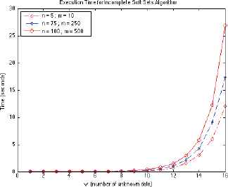
Matlab implementation performance of our Algorithm. For convenience we partially display the data in Table 8.
| # unknown values | Matrix Dimensions (n,m) |
||||
|---|---|---|---|---|---|
| (5,10) | (25,100) | (50,200) | (75,250) | (100,500) | |
| 1 | 0.0008 | 0.0009 | 0.0009 | 0.0011 | 0.0018 |
| 2 | 0.0012 | 0.0014 | 0.0014 | 0.0014 | 0.0029 |
| 3 | 0.0017 | 0.0024 | 0.0025 | 0.0028 | 0.0050 |
| 4 | 0.0032 | 0.0038 | 0.0048 | 0.0049 | 0.0075 |
| 5 | 0.0056 | 0.0068 | 0.0088 | 0.0093 | 0.0126 |
| 6 | 0.0109 | 0.0127 | 0.0148 | 0.0174 | 0.0271 |
| 7 | 0.0226 | 0.0244 | 0.0301 | 0.0318 | 0.0460 |
| 8 | 0.0446 | 0.0490 | 0.0584 | 0.0702 | 0.1004 |
| 9 | 0.0926 | 0.0959 | 0.1157 | 0.1542 | 0.2041 |
| 10 | 0.1836 | 0.1926 | 0.2331 | 0.2844 | 0.4128 |
| 11 | 0.3782 | 0.3879 | 0.4726 | 0.5603 | 0.8252 |
| 12 | 0.7535 | 0.7700 | 0.9245 | 1.0916 | 1.5072 |
| 13 | 1.5563 | 1.5493 | 2.0415 | 2.1525 | 2.9577 |
| 14 | 3.0519 | 3.0954 | 3.8883 | 4.2896 | 5.8508 |
| 15 | 6.0364 | 6.2123 | 7.3964 | 9.0436 | 12.2864 |
| 16 | 12.1147 | 13.2758 | 15.4481 | 17.3812 | 26.9188 |
Matlab implementation performance of our Algorithm: running times in seconds.
For larger sets of data, experimental analyses become tediously lengthy. Consequently, Figure 2 is a logarithmic representation analogous to Figure 1 of the same cases (a), (d), and (e) *. However, in this graph instead of using 10 random matrices, we only consider three experiments for the sake of minimizing execution time.
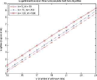
Matlab implementation performance of our Algorithm. For interpretation of the data, see Section 4.
In all series we found that the running time of the Algorithm is exponential to the number of unknown elements in the matrix. For example, we tested it for a matrix with n = 100, m = 500, and w = 30 and the execution time was 2.2848 · 105 seconds (= 63,46 hours = 2.64 days) with the same basic computer.
We must acknowledge that when the value of w grows above a certain level, the running time makes the Algorithm impracticable as it stands. But that level does not seem to be surpassed in the literature we have sampled. In this regard it seems convenient to compare our proposal where every missing data are either 0 or 1, with other possible studies where the incomplete infomation is filled with numbers ranging in a larger set. We believe that even if the researcher attempts to estimate the missing data, the majority of the approaches restrict the options to 0 or 1 (cf., DFIS in Qin et al. 22, ADFIS in Khan et al. 26, and Qin et al. 21). As an exceptional case where larger sets of values can be used, we can only cite the recent Kong et al. 16 (see their Tables 4, 7 and 12).
4. Final Comments and Conclusion
Our proposal provides a new criterion for soft set based decision making problems under incomplete information. We have demonstrated that this method is different from the approaches in the existing literature.
The main advantage of our work is that under the conditions in which there is no inherent relationship between objects and between parameters, the decision result will be more convincing than other approaches. In the general framework where no such information on relationships is available, the user must avoid the recourse to possible similarities between objects and/or parameters that are the premise of other approaches. According to Laplace’s principle of indifference, in case of complete ignorance we are entitled to assume that all tables in which the ∗’s are replaced with either 0 or 1 are equiprobable. In each of these cases it is reasonable to compute the objects selected according to soft-set based decision making in order to make a decision that is optimal in the highest proportion of cases.
In view of the computational analysis in subsection 3.5, in our future investigations we will focus on related algorithms that permit to preserve the ethos of our approach and take on the cases that require a large execution time.
The following two techniques can be used for that purpose.
- 1.
The researcher can select a random sample out of the 2w possible matrices in such way that with a sufficiently large number of samples, the estimate
This procedure is efficient since it can be stopped at any time. The verdict as to which options are optimal is adjustable because it depends on the proportion of filled tables that are used. This main feature is common to other approaches (e.g., the use of thresholds in Qin et al. 21 in this context; or the adjustable approach by Feng et al. 11 in fuzzy soft set based decision making). The choice of the thresholds in the latter proposals is under the control of the users, and the technique in Alcantud and Santos-García 4 leaves the decision of such proportions to the users too.
- 2.
One can produce a modification of our idea in subsection 3.3 that exploits the fact that when there are several missing data for an option, the result of its choice value does not depend on the precise alternatives that are completed with a 1, but rather it is dependent on the exact number of alternatives that are completed with a 1, since the choice value is computed by addition. Hence, our Algorithm can be refined to run in less time by replacing Steps 4 and 5 with a better procedure that goes through all the possibilities and computes how many times each case takes place. We emphasize that a non-trivial combinatorial problem emerges.
Finally, it would be interesting to extend our approach to the theories formulated by Han et al. 14 regarding decision making of incomplete soft sets generated by restricted intersection.
Table 4 summarizes the techniques available to the practitioner for the problem we have studied.
| Method(s) and tool(s) | Indexes | Ref. | Comments | |
|---|---|---|---|---|
| Weight-average of all possible choice values of objects Weights of each choice value given by distribution of the other objects |
di, di−p, ci(0), ci(1) |
36 | Original approach | |
| Data filling based on association between parameters Choice from choice values for completed set |
Qi | 21 | Proposed here. Suitable for cross-related objects Inspired by 36 |
|
| Elicitation criterions for incomplete soft sets generated by restricted intersections | - | 14 | Different approach to related problem | |
| Elimination of dominated options Laplacian argument: equal probability to all completed tables Choice mechanism: choice values |
Random sample |
|
4 | Results depend on sample † Sample size under control of user |
| Brute force | si | Alg. 1 | Computationally costly for sizes larger than problems in applied literature † | |
| Combinatorics | - | - | Future research † | |
Suitable when there is no guarantee that objects and parameters are related to each other.
Summary table of studies about incomplete soft set based decision making.
Acknowledgment
We gratefully acknowledge the helpful comments made by two anonymous referees and by Luis Martínez, Editor-in-Chief. The research of Santos-García was partially supported by the Spanish projects Strongsoft TIN2012–39391–C04–04 and TRACES TIN2015–67522–C3–3–R.
Footnotes
We use logarithmic representations in order to avoid extreme distortions in the graphical display.
References
Cite this article
TY  - JOUR
AU  - José Carlos R. Alcantud
AU  - Gustavo Santos-García
PY  - 2017
DA  - 2017/01/01
TI  - A New Criterion for Soft Set Based Decision Making Problems under Incomplete Information
JO  - International Journal of Computational Intelligence Systems
SP  - 394
EP  - 404
VL  - 10
IS  - 1
SN  - 1875-6883
UR  - https://doi.org/10.2991/ijcis.2017.10.1.27
DO  - 10.2991/ijcis.2017.10.1.27
ID  - Alcantud2017
ER  -