
Using ANNs Approach for Solving Fractional Order Volterra Integro-differential Equations
- DOI
- 10.2991/ijcis.2017.10.1.32How to use a DOI?
- Keywords
- Fractional equation; Power-series method; Artificial neural networks approach; Criterion function; Back-propagation learning algorithm
- Abstract
Indeed, interesting properties of artificial neural networks approach made this non-parametric model a powerful tool in solving various complicated mathematical problems. The current research attempts to produce an approximate polynomial solution for special type of fractional order Volterra integro-differential equations. The present technique combines the neural networks approach with the power series method to introduce an efficient iterative technique. To do this, a multi-layer feed-forward neural architecture is depicted for constructing a power series of arbitrary degree. Combining the initial conditions with the resulted series gives us a suitable trial solution. Substituting this solution instead of the unknown function and employing the least mean square rule, converts the origin problem to an approximated unconstrained optimization problem. Subsequently, the resulting nonlinear minimization problem is solved iteratively using the neural networks approach. For this aim, a suitable three-layer feed-forward neural architecture is formed and trained using a back-propagation supervised learning algorithm which is based on the gradient descent rule. In other words, discretizing the differential domain with a classical rule produces some training rules. By importing these to designed architecture as input signals, the indicated learning algorithm can minimize the defined criterion function to achieve the solution series coefficients. Ultimately, the analysis is accompanied by two numerical examples to illustrate the ability of the method. Also, some comparisons are made between the present iterative approach and another traditional technique. The obtained results reveal that our method is very effective, and in these examples leads to the better approximations.
- Copyright
- © 2017, the Authors. Published by Atlantis Press.
- Open Access
- This is an open access article under the CC BY-NC license (http://creativecommons.org/licences/by-nc/4.0/).
1. Introduction
Fractional calculus is old subject but it recently has found numerous applications in various fields of science and engineering 1,2,3,4,5,6. Fractional derivatives are powerful and efficient tools to describe the physical systems that have long-term memory 7,8. Especially, in modeling the complex dynamic systems it can be seen that fractional differential equations naturally arise once power-type non-local interacting systems with power-law memory 5,9,10. Differential equations of the fractional order have gained applications in modeling non-conservative systems 11,4. A large amount of research works has been devoted to tackle a wide variety of fractional equations, particularly generalized odd dimension mechanics is suggested in Refs 12,13,14,15.
The analytical and approximate analytical methods are used to achieved the solutions of differential equations 16. The fractional deferential equations are solved using generalized analytical, approximate analytical methods and numerical methods17,6. The iterative methods is utilized widely and found the solution of the equations in the area of the initial and boundary value problems. We already have a number of famous computational techniques dealing with the solution of high order fractional differential equations, such as weighted essentially non-oscillatory scheme 18, Chebyshev collocation method 19,20, Green functions method 21 and block-by-block approach 22. Moreover, as an excellent modeling tool, fractional integro-differential equations issue have attracted much attention recently 23,24.
The artificial neural networks (ANNs) approach has attracted much consideration to its advantages, such as learning, adaptivity, fault-tolerance, etc 25,26,27,28. Recently, a modification of ANNs approach has been developed to the treatment of related boundary problem in two-dimensional case . On the other hand, power series method has received considerable attention in dealing with complicated math problems. This method provides the solution function as a series polynomial in which its coefficients can be determined via an appropriate standard method. Here, we intend to extend the application of neural networks approach and power series method as an iterative minimization strategy for the numerical solution of the mentioned fractional order initial value problem. It is worthy of note that, representation of solution in terms of a suitable truncated series expansion is the fundamental issue in approximation theory. After discretizing the problem domain into elements and making substitutions, the mentioned equation is transformed to minimizing problem by using the least mean square (LMS) error function. Now, the generalized delta learning rule is used to minimize the mentioned error function on the unknown space. After determining the unknowns, the solution can be calculated via a convergent series polynomial 29.
The brief outline of this paper consists of the following steps:
Current research begins the procedure in section 2, by reviewing basic definitions and fundamental issues of neural networks and fractional calculus. Here, the given initial value problem is also investigated via the offered combination numerical method. Two numerical examples are given in section 3 to show that our method yields accurate approximates of the mentioned problem. Since, the mentioned problem usually has no exact solution in the fractional order, the obtained numerical results can not be compared with exact ones. So to have the better understanding of the method, we help the error caused by the proposed method, and we show that by growing the number of iterations, this error is reduced. Finally, conclusion is described in section 4.
2. Description of the Method
As indicated, unique capabilities of artificial neural networks have persuaded researchers to serve these as powerful tools in solving complex real world problems. The main aim of this section is to combine the ANNs approach and a modification of polynomial series technique as an efficient iterative method to approximate numerical solution of a linear Fredholm integro-differential equations of fractional order. In order to better clarify all the fundamental mathematical features of the method presented in this research, first some preliminary definitions and necessary notations in neural networks are given, which will be utilized in the following parts.
2.1. Basic Idea of ANNs
First, let us have a brief part of introduction on typical neural networks. The most striking question about neural networks is why they have been applied. To gain insight into this question, we go through the paper and also we will explore the reasons why they are useful for solving certain types of tasks and it is believe that algorithmic and math problems are solved by computers which are as a specific piece of technology. It is sometimes seen that there are likely a lot of failed mathematical algorithm. There are a couple of problems that are not effortless to be expressed into an algorithm such as facial recognition and language processing. However, these tasks are trivial to humans. One important and pioneering feature of artificial neural networks is that their design enables them to process data in a similar way to our own biological brains which is done by drawing inspiration from the form of our own nervous system functions. This qualifies them more sophisticated at solving problems like facial recognition, which our biological brain is capable of doing it easily. We also do a good job understanding of operating the designed neural network and processing data. An Artificial neuron is conceived as a model of biological elements (neurons). There are many References on neural nets field 25,26.
Figure 1, illustrates a widely used structure consisting of a external input and one hidden layer of the identity activation type which are completely interconnected to a single linear output neuron. It is worth mentioning that there can be any number of limited edition series of nodes per layer and there is exactly one hidden layer to pass through before reaching the output layer. It is needed to say that if an appropriate number of nodes and layers could be chosen during optimizing, neural network would be implemented appreciatively. In the diagram shown, since the signals are passed through the layers of the neural network in a single direction, this diagram is called a feed-forward back-propagation network. Here, output unit can travel into the opposite direction to input signals. In this paper, we introduced an additional adaptive multi-layer neural network and its significant qualities. In the following, the designed architecture will be considered which is capable of approximating solution of the mentioned nonlinear math problem, to any desired degree of accuracy. As the model is running, training patterns from each input signal are weighted and then introduced into the hidden layer, where they are summed and passed through given activation functions. By computing the resulting values are weighted and summed to be the networks output. Assume that the parameters vi,wi (for i = 1,..,n) and b denote the corresponding connection weights and bias term, respectively. According to the above, the relations in each neuron of proposed network structure can be expressed as follows:
- •
Input unit:
- •
Hidden units:
- •
Output unit:
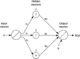
Block diagram of the represented neural architecture.
The most important issue is that is that the designed neural network will not be able to perform the given target by itself. Therefore, we must adopt a procedure that given the network parameters to be adjusted in order to achieve the ultimate goal. There are many effective ways which help us to achieve this goal. One of the famous methods is the back-propagation learning algorithm. The mentioned learning algorithm was fully introduced in 1986 by Rumelhart and Mc-Clelland 30. The concept of forward propagation is that the given artificial neurons are located in network layers, and then generate its signal output to forward direction. Back-propagation which is a supervised algorithm means that the errors back must be propagated to adjust the weighs and bias parameters. For this aim, the calculated output is compared with the desired one, and then network error can be calculated via a suitable rule easily. In this algorithm it is assumed that the network parameters have been randomly quantified with small real valued numbers. Now, at each learning step the network output is calculated and it looks for the minimum of the error function. To the better approximation, a combination of introduced neural network mathematical modeling technique with a modification of power series method will be described in the following parts of paper.
2.2. Implementation of the method
Increasing use of fractional problems modeled by integro-differential equations (IDEs), has led to the development of new research on these mathematical problems. As previously indicated, many different algorithms are available to the numerical solutions of differential equations of fractional order. Due to the power series method’s computation productivity and less storage requirements, it seems to be the most commonly used one in modeling fractional problems. In the work mentioned here, we focus on the numerical solution of mentioned initial value problem via a combination of neural nets approach and power-series method.
Let us recall notations and some general concepts regarding fractional calculus that are significant in this study 1,2,3,4,5,6.
Definition.
If u(x) is continuously differentiable function on interval [a,b] up to order k. Then the Caputo derivative
In the above relations, notation ⌈ α ⌉ is denoted the smallest integer greater than or equal to constant α 1,2,3,4,5,6. Now, we intend to solve the following linear Volterra integro-differential equation of fractional order:
2.2.1. Discretization of the problem
Often, finding an analytical technique really is pretty impossible to determine the exact solutions of applied mathematical problems. The power series solution method has been traditionally developed by several authors, as an approximate but theoretically acceptable method to solve most variety of differential equations. In other words, capacity of power series to introduce any analytical function with algebraic series is coming up with the idea of developing approximate solution. The method considered here aims to produce a specific solution with a series of unknown coefficients. Ones, the power series polynomial is substituted in given differential problem, a system of equations is provided in linear or non-linear case. Now, ANNs approach is employed to obtain the initial or boundary value based unknown coefficients. This procedure will lead us to approximate unknown functions for the solution coefficients. Note that existence, particularity and smoothness of the solution are well defined.
The proposed combination method first consists of substituting solution in the decomposition form given by:
It should be considered that the proposed test function (10), must be satisfied in the corresponding initial conditions. In order to subdue this imperfection, the series solution is modified by:
It is reasonable to consider that the designed feed-forward neural net is fully associated with the first (n + 1) terms of series (11). The offered architecture satisfies by construction the given initial condition, and also contains unknown coefficient in which to be determined. Assuming that utrial(x) symbolizes the trial solution with adjustable parameters aj, the problem is transformed from the original construction to an unconstrained one by direct substitution (11) in (8). Thus, we have:
Now, a set of acceptable node points must be defined for the discretization of resulting equation. Let an uniform partition on domain [0,T] with the node points
In the following part, we will review the iterative technique which help us to solve the resultant system for unknown coefficients.
2.2.2. Proposed error function
The conventional way in artificial neural networks approach is to start with an initial neural architecture with untrained network parameters (weights and biases), presentation training patterns to calculate the corresponding neural outputs and then employing an error correlation rule to update the parameters at every stage of repetition. The error correlation rule is a suitable combination of a given criterion function of the weights and bias parameters and an efficient learning algorithm that minimizes the criterion function for the set of connection weights and biases. In other words, the network parameters are adjusted to reduce the network error. The least mean square (LMS) output error which is a quadratic error correcting rule, represents the most commonly used criterion function 33. Here, one starts with the indicated criterion function as follows:
Then the total error is obtained by summing the predetermined error function over all the collocation points, as:
Eventually, an attempt is made to the adjustment of network parameters through an efficient learning algorithm. In other words, we intend to employ the training rules for minimizing the network error by adaptively updating the network parameters. In order to achieve this goal, one possible error correction rule as the steepest gradient descent based back-propagation algorithm must be essentially used to optimize the weight terms. Further details in this respect can be found in 34.
2.2.3. Proposed learning algorithm
Learning in neural networks is choosing the appropriate network parameters where the total network error is minimized by using each training pattern. Now, the well-known back-propagation algorithm lies in and calculates to detect how much the network error depends on the input signals, network output and connection weights. To learn, first the input signals are quantified by arbitrary initial guesses, and then neural network will calculate the output for each training set. Then, the defined LMS error function is employed to train the proposed network. So, we use an optimization technique which in turn requires the computation of the gradient of the error with respect to the net parameters. finally, the supervised back-propagation learning algorithm is used for adjusting the parameters such that the network error to be minimized with respect to the input signals. The performance of this algorithm is well summarized in the following paragraph.
Now, the initial network parameters aj (for j = 1,…,n) are chosen randomly to begin the learning process. The weight change for any hidden layer parameter aj can thus be written as:
It is clear that existing a mathematical software with high quality will be necessary to omit wasting time and enhance the accuracy of complicated calculations. In this study, the presented numerical examples have been tested with mathematical programing software Matlab v7.10.
3. Numerical Simulation and Discussion
To illustrate the ability of the method outlined in the previous section, it was applied to the two fractional order initial value integro-differential equations. Also, in order to confirm whether the mentioned iterative technique leads to higher accuracy, the test cases are compared in simulation with the samples provided in 35. Below, we use the formal specifications η = 0.03 and γ = 0.05.
Example 3.1.
Consider the following fractional order linear Volterra integro-differential equation:
| Variable | Description |
|---|---|
| n | The order of power-series polynomial |
| n′ | The number of collocation points |
| t | The index of iterations |
| xr | The training locations |
| γ | Momentum constant |
| r | The training index |
| η | Learning rate |
| E | Total error |
First, the initial output-layer connection weights ai (for i = 1,…,n) are quantified with small random values, which have been chosen randomly on interval [0,1]. Then the training patterns are used to successively adjust the connection weights until a suitable solution is found. To illustrate the more efficiency and to have the highest view of this method, the indicated root mean square error is shown in Table 1. It can be seen that by increasing the learning steps, total error decreases. The error function has been plotted in Figure 2 for t = 300 and n′ = 3.
Criterion function on the number of iterations.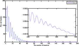
| t | − − − − − − n = 3 − − − − − − | ||
| n′ = 10 | n′ = 15 | n′ = 20 | |
| 500 | 8.7512 × 10⁻⁸ | 7.0881 × 10⁻⁸ | 5.9311 × 10⁻⁸ |
| 1000 | 6.2704 × 10⁻⁸ | 2.3801 × 10⁻⁸ | 2.1466 × 10⁻⁸ |
| 2500 | 3.4298 × 10⁻⁸ | 2.1701 × 10⁻⁸ | 1.9033 × 10⁻⁸ |
| 5000 | 2.6809 × 10⁻⁸ | 1.8378 × 10⁻⁸ | 1.2571 × 10⁻⁸ |
| t | − − − − − − n = 5 − − − − − − | ||
| n′ = 10 | n′ = 15 | n′ = 20 | |
| 500 | 5.4431 × 10⁻⁸ | 4.8669 × 10⁻⁸ | 4.0364 × 10⁻⁸ |
| 1000 | 3.9018 × 10⁻⁸ | 3.7442 × 10⁻⁸ | 2.3472 × 10⁻⁸ |
| 2500 | 3.2436 × 10⁻⁸ | 3.3325 × 10⁻⁸ | 2.0022 × 10⁻⁸ |
| 5000 | 2.6972 × 10⁻⁸ | 2.0172 × 10⁻⁸ | 8.7112 × 10⁻⁹ |
| t | − − − − − − n = 7 − − − − − − | ||
| n′ = 10 | n′ = 15 | n′ = 20 | |
| 500 | 4.2369 × 10⁻⁸ | 3.5371 × 10⁻⁸ | 3.1022 × 10⁻⁸ |
| 1000 | 2.4365 × 10⁻⁸ | 2.1914 × 10⁻⁸ | 1.8439 × 10⁻⁸ |
| 2500 | 1.7230 × 10⁻⁸ | 1.1920 × 10⁻⁸ | 8.6610 × 10⁻⁹ |
| 5000 | 1.1301 × 10⁻⁸ | 9.0748 × 10⁻⁹ | 7.2301 × 10⁻⁹ |
| t | − − − − − − n = 9 − − − − − − | ||
| n′ = 10 | n′ = 15 | n′ = 20 | |
| 500 | 3.4383 × 10⁻⁸ | 2.1633 × 10⁻⁸ | 1.9175 × 10⁻⁸ |
| 1000 | 6.4571 × 10⁻⁹ | 3.2133 × 10⁻⁹ | 2.2344 × 10⁻⁹ |
| 2500 | 4.1745 × 10⁻⁹ | 2.8889 × 10⁻⁹ | 1.4580 × 10⁻⁹ |
| 5000 | 3.8311 × 10⁻⁹ | 2.0716 × 10⁻⁹ | 1.2172 × 10⁻⁹ |
Measured total network errors for different number of network parameters.
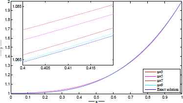
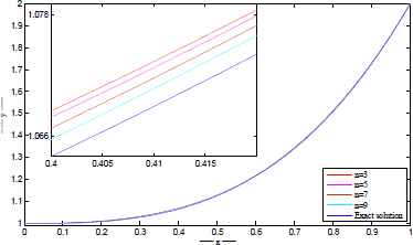
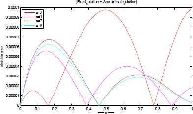
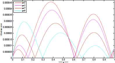
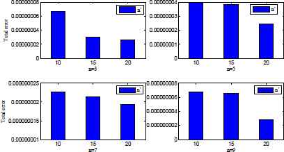
The exact and approximate solutions are plotted in Figures 3–6 for different number of network parameters. Also, the absolute error between approximate and exact solutions are plotted in Figures 7–10 for different number of network parameters. Moreover, the relationship between the increasing of output neurons, training nodes and the performance analyzing of introduced ANN is given in Figure 11.
Exact and approximate solutions for t=500. Exact and approximate solutions for t=1000. Exact and approximate solutions for t=2500. Exact and approximate solutions for t=5000. |u(x) − utrial(x)| for t=500. |u(x) − utrial(x)| for t=1000. |u(x) − utrial(x)| for t=2500. |u(x) − utrial(x)| for t=5000. The performance of proposed network architecture over different neural elements for t = 5000.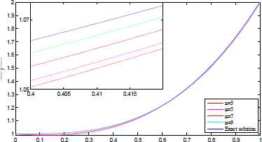


Example 3.2.
As the second example, consider the following initial value fractional problem:
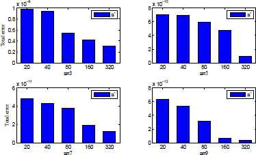
The performance of proposed network architecture over different neural elements for t = 5000.
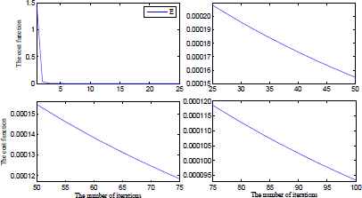
The cost curve for n = 3, n′ = 320 and t = 100.
| n′ | ANN | ||||
| −−−−−−−−−−−−−−−−−−−−−−−−−−−−−− | |||||
| n = 3 | n = 5 | n = 7 | |||
| 20 | 0.9813 × 10⁻⁸ | 0.7101 × 10−09 | 0.4738 × 10⁻¹⁰ | ||
| 40 | 0.9225 × 10⁻⁸ | 0.6967 × 10−09 | 0.4141 × 10⁻¹⁰ | ||
| 80 | 0.5140 × 10⁻⁸ | 0.5838 × 10−09 | 0.3944 × 10⁻¹⁰ | ||
| 160 | 0.2780 × 10⁻⁸ | 0.4417 × 10−09 | 0.1919 × 10⁻¹⁰ | ||
| 320 | 0.2184 × 10⁻⁸ | 0.8660 × 10⁻¹⁰ | 0.1133 × 10⁻¹⁰ | ||
| n′ | ANN | HC | |||
| −−−−−−−−−−−−−−−−−−−−−−−−−−−−−− | |||||
| n = 9 | |||||
| 20 | 0.6238 × 10⁻¹¹ | 0.2878 × 10⁻⁵ | |||
| 40 | 0.4638 × 10⁻¹¹ | 0.8731 × 10⁻⁶ | |||
| 80 | 0.3170 × 10⁻¹¹ | 0.3952 × 10⁻⁶ | |||
| 160 | 0.8719 × 10⁻¹² | 0.1706 × 10⁻⁶ | |||
| 320 | 0.4815 × 10⁻¹² | 0.8344 × 10⁻⁷ | |||
Obtained numerical results for t = 5000.
4. Conclusion
Through the use of power series method and neural networks approach, a combination iterative technique has been derived for finding solution of an initial value linear Volterra integro-differential problem involving fractional order. The process begins with the assumption that the unknown function can be expressed as a power series polynomial. In this regard, the mentioned fractional problem is reduced to solve a linear algebraic equations system. Then, a modification of ANNs approach is employed to the comparative study of achieved system. The suggested technique was applied to study two test cases of the problem. The obtained results showed that the employed neural architecture is powerful mathematical tool for solving mentioned type integro-differential equation. Also, we compared the obtained results with both their exact solutions and those of another numerical method. The given numerical examples support our claim that the employed neural architecture gives rapidly convergent approximation without any restrictive assumptions. As areas for future research, extension of this method can be extended to cover nonlinear fractional integro-differential equations.
References
Cite this article
TY  - JOUR
AU  - Ahmad Jafarian
AU  - Fariba Rostami
AU  - Alireza K. Golmankhaneh
AU  - Dumitru Baleanu
PY  - 2017
DA  - 2017/01/01
TI  - Using ANNs Approach for Solving Fractional Order Volterra Integro-differential Equations
JO  - International Journal of Computational Intelligence Systems
SP  - 470
EP  - 480
VL  - 10
IS  - 1
SN  - 1875-6883
UR  - https://doi.org/10.2991/ijcis.2017.10.1.32
DO  - 10.2991/ijcis.2017.10.1.32
ID  - Jafarian2017
ER  -