1. Introduction

Optical networks employing wavelength division multiplexing (WDM) and wavelength routing techniques are being considered as a candidate solution for future backbone infrastructures ¹. Such networks are able to provide practically unlimited bandwidths required for a variety of advanced and upcoming telecommunication services and applications. With the purpose to offer high data rates and guaranteed quality of service to end users network operators (NOs) have to provide a number of connections over optical network infrastructure. All-optical connections established between two wavelength routing nodes are called the lightpaths. While establishing the lightpaths a NO tries to maximize its own revenue by charging the occupation of network resources. To achieve this goal NO has to be addressed how to solve the call admission control jointly with the lightpaths routing and wavelength assignment (RWA) problem¹. Various services over future backbone optical networks, like lambda grids or optical virtual private networks (oVPNs) could be characterized as off-line (or static) traffic demands. In such case, the traffic demands are specified in advance before the connections have to be established. By knowing the complete set of demands, a more efficient network resource usage (and consequently more revenues) could be achieved compared to on-line (dynamic) traffic case in which future demands are not known a priori.

So far, various approaches to solve the revenue (profit) maximization problem in optical WDM networks have been proposed in literature ^2–6. In Ref. 2, the problem of maximizing profits is mathematically formulated as an integer linear programming (ILP) problem. Since the optimal provisioning of lightpaths is NP-hard combinatorial problem, several heuristic algorithms are proposed to solve the problem assuming both an off-line and an on-line traffic model. The authors of Ref. 3 proposed an efficient near-optimal algorithm based on Lagrangean relaxation (LGR) approach to solve the lightpath provisioning problem in which the revenue from accepting call requests is to be maximized. In Ref. 4 a polynomial-time algorithm to design a k-colourable set of paths in a chain WDM topology as well as 2-approximation algorithm for ring topology are proposed, such that the total profit of the set of designed paths is maximized. In Ref. 5, the authors propose a heuristic algorithm based on the genetic algorithm (GA) approach for addressing the problem of optimal provisioning of virtual network requests with unsplittable and splittable flows in cloud-based data centres such that total revenue is maximized. Following recent advancing in optical technology, the authors of Ref. 6 proposed two wavelength assignment approaches for flex-grid optical path topology, with the goal to maximize the total profit.

In this paper, the bee colony optimization (BCO) metaheuristic is applied to solve the revenue maximization (or shortly Max-Rev) problem in optical WDM networks. Various studies proved that BCO is a fast, robust and efficient optimization tool, which can produce high quality solutions together with small computational complexity^7–15. A comprehensive overview of BCO metaheuristic with its various applications could be found in Refs. 10 – 11. Inspired by a number of successful previous BCO implementations, our goal here is to demonstrate the quality and efficiency of the BCO approach while solving the considered Max-Rev problem. To the best of our knowledge, this study is the first application of the BCO approach to solve the revenue optimization problem in communication networks. Previous results have proved that BCO could be better-quality approach compared to other heuristic and metaheuristic algorithms. It indicates that BCO could be a promising candidate to solve various complex optimization problems in WDM optical networking, such as the considered Max-Rev problem.

The main contributions of this paper are following:

1. i)

   We adapted the BCO model previously proposed in Ref. 9 to solve the considered Max-Rev problem in optical WDM networks. Although the objective in Ref. 9 is to maximize the number of established lightpaths, it does not consider the economic aspects, which are highly important from network operator’s point of view. However, it is obvious that maximizing only the number of established lightpaths does not necessarily imply the maximal NO’s revenues, too. The exception is the scenario where all the lightpaths are equally charged, which is not too realistic case. Hence, the optimization task is to make a decision what is the best set of lightpath demands to be established together with their routes and wavelengths, such that the total NO’s revenue is maximized under the limited available wavelengths in a given WDM network.

2. ii)

   We developed an entirely new Max-Rev optimization model by implementing the improvement BCO approach (shortly, BCOi). BCOi is a more recent approach that is firstly proposed in Ref. 12 to solve the well-known p-centre problem in graph theory. It will be shown that our Max-Rev BCOi algorithm is able to produce near-optimal (or even optimal) solutions, which are superior compared to the constructive version of the BCO-model⁹ as well as to some simple heuristics, such as the Max-Profit and first-come-first-served (FCFS) algorithms proposed in Ref. 2.

3. iii)

   In addition, we have applied the differential evolution (DE) metaheuristic to the considered Max-Rev problem in order to perform a more reasonable comparison of BCOi to other similar optimization approaches. DE is a population based random search technique, which performs iteratively through a number of generations to find the best solution to the problem. Like the GA approach, DE also uses evolutionary operators (mutation, recombination and selection) to modify the population of individuals (set of candidate solutions) in each generation. The main control parameters of DE are: the mutation constant (M), which controls the mutation strength; the recombination constant (RC), which increases the diversity in the mutation process; and the population size (NP) that is an integer that depends on the dimension of the problem.^16–19 DE searching procedure starts with a randomly created initial population and iterates by creating new populations until a given stopping criterion is satisfied. A more comprehensive theoretical description of the DE approach could be found in Ref. 16. Several studies in optical networking show that DE outperforms some other evolutionary algorithms ^17–19. However, it has been recently shown in Ref. 20 that BCOi is superior compared to DE as well as to particle swarm optimization (PSO) metaheuristics in terms of the solution quality and the efficiency while solving the wavelength converters placement problem in WDM networks. This encouraged us to choose the BCOi as an efficient tool to solve the Max-Rev problem in this paper.

The paper is organized as follows. In Section 2, the statement of the Max-Rev problem is given. The main principles of the BCOi metaheuristic are described in Section 3. The proposed BCOi model for solving the considered Max-Rev problem is introduced in Section 4. In Section 5, we demonstrate the numerical results of performance study and comparisons under various WDM optical network topologies. Finally, some conclusions are given in the last section.

2. Max-Rev Problem Statement

We consider an optical WDM physical network topology that consists of set of network nodes N (equipped with optical cross-connects), which are interconnected by set of optical links L in an arbitrary (mesh) topology. We make the following assumptions: every link in a physical optical network consists of a pair of optical fibres; each fibre has the same set of available wavelengths W; wavelength converters are not available at network nodes, hence the wavelength continuity constraint has to be satisfied; there is no limitation on the number of optical transceivers at network nodes; each lightpath is exclusively used for one source-destination node pair (s,d); the set of requested lightpath demands K as well as the set of candidate shortest paths P_k for each lightpath demand are given in advance. Each lightpath demand is specified by its starting and ending time during a (short) planning horizon. Such situation could be usually found in practice when there is no need to establish the lightpaths for an infinite duration, but rather for a particular period during a day (for example several hours) or for some other periods. We assumed also that every lightpath demand contributes to different NO’s revenue. The revenue for a lightpath could depend on various aspects, such as for example the geographical distance between wavelength routing nodes, duration of a lightpath, time periods during a planning horizon, requested priority of a lightpath demand, quality of service parameters etc. For simplicity, we assume here that revenue for a lightpath depends on its duration and the period during a planning horizon (for example, NO could offer lower prices during the periods of light traffic demands and higher prices during busy hours). Hence, we define the revenue R_k for establishing a lightpath demand k as follows:

Under the above assumptions, the considered Max-Rev problem could be expressed as follows: for given optical WDM physical network topology, traffic demands and number of wavelengths on WDM links, the objective is to determine the best (optimal) set of lightpaths to be established jointly with their routes and assigned wavelengths such that total NO’s revenue is maximized. To find the optimal solution of the considered problem, we used the integer linear programming (ILP) formulation proposed in Ref. 3. The rest notations used in this formulation are following:

constants:

• δpl={1, if path p∈Pk includes link l∈L,0, otherwise

  T

  − set of time events (for detail insight of time events see Ref. 3),

  σkt={1, if lightpatk k∈K includes even time t∈T,0, otherwise

binary variables:

• xpwk={1, if a lightpath k∈K traverse path p∈Pk   using the wavelength w∈W,0, otherwiseyk={1, if a lightpath k∈K is established0, otherwise

Following is the mathematical (ILP) formulation of the considered Max-Rev problem ³:

The objective function, given by Eq. (2) is to maximize the total revenue for a NO. It could be noticed that in a special case, when all lightpath demands have the same revenue R_k=1, the considered ILP formulation is reduced to the problem of maximization the number of established lightpaths. The constraints (3) to (4) ensure that mostly one lightpath should be established for each traffic demand. Constraints (5) prevent wavelength conflicts, i.e. ensure that on every link only one wavelength (lightpath) could be used at any time slot. Constraints (6) and (7) ensure that corresponding binary variables could take only one value (0 or 1). A binary value of variable in constraints (7) determines if the lightpath demand is established (y_k=1) or not (y_k=0). The ILP formulation is shown to be NP-hard optimization problem that could be solved exactly only in case of small problem dimensionality. However, ILP becomes computationally intractable even for moderately large networks or incurs a large computational time to find the optimal solution. Hence, heuristic based approaches should be used to find the (suboptimal) solution. We used here the BCOi metaheuristic approach to solve the considered optimization problem in case of realistic size optical WDM networks. Before presenting the BCOi implementation for considered Max-Rev problem, we present shortly the main principles of BCO metaheuristic in following section.

3. BCO Main Principles

BCO metaheuristic is a population based stochastic random-search technique that is inspired by the foraging habits of natural bees looking for nectar sources ^8–15. It is originally proposed by Teodorović and Lučić in Ref. 14.

Similar to the foraging habits of natural bees, the artificial bees in BCO perform the examination of the search space looking for the best solutions. Each bee in a population generates one solution to the considered optimization problem.^7–15

During the iterative searching procedure, bees generate (or improve) its individual solutions yielding to new ones. In order to find the best solution, artificial bees perform cooperative decisions in the hive by exchanging the information about the quality of their current solutions. In this way, bees progressively discover solutions that are more promising and gradually leave worse ones. There are two approaches of the BCO metaheuristic ^10,11: the constructive BCO and the improvement (BCOi) versions. The first approach is based on constructive steps in which bees begin to search for the best solution from an empty solution and incrementally expand their solutions during the search process. In the improvement (BCOi) approach bees start with a complete initial solution of the considered problem and modify it through the search process in order to obtain the best possible final solution. We used the second (BCOi) approach in this study.

As it is already mentioned, the searching procedure in BCO algorithm is performed iteratively ^10,11. Each iteration contains a number of steps (S) and each step consists of the so called forward pass (FP) and backward pass (BP), which are performed alternatively. The number of forward/backward passes (or steps S) is specified in advance. In each forward pass, every bee makes a number of modifications (M) of its current solution. At the beginning of search process, all artificial bees are placed in the hive. The number of bees (B) engaged in the search process is specified in advance, too. An illustration of the first forward and backward pass is shown in Fig.1 (a). To simplify the illustration, we assumed that there are B=6 bees in the hive. At the beginning of search process bees start the searching from an initial complete solution that could be generated randomly or by applying some heuristic algorithm. By knowing the initial solution, all bees start to fly through the search space and modify the current solution trying to improve it in each step. During a forward pass every bee flies through several stages (which are represented by flowers in Fig. 1).

Fig. 1.

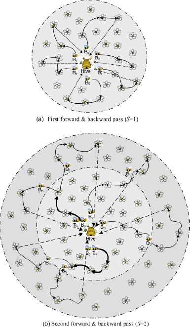
Illustration of: a) the first (S=1) and (b) the second (S=2) forward and backward passes

In each stage, every bee modifies its current solution compared to the previous stage yielding to a new solution.^10–13 The number of solution modifications (M) within each forward pass (FP) could be specified in advance or randomly chosen at the beginning of each forward pass. After M modifications of solutions performed by all bees, the first forward pass is finished and the second phase of the BCO step, the so-called backward pass (BP) begins. During the BP, all bees fly back to the hive (it is illustrated by straight dash lines in Fig.1) in order to share information and compare the quality of generated solutions. The quality of bee’s solution corresponds to the considered objective function value. It is assumed that each bee in the hive could be aware of its own solution quality and at the same time, she can obtain the information about solutions’ quality of all other bees. By exchanging the information about the quality of individual solutions, every bee has to decide whether it will be loyal to its individual solution or not ⁸. Such decision is made with a certain probability such that the bees with better solution quality (objective function value) have more chances to keep their solutions. The bees that are loyal to their solutions create the set of recruiter bees, while the other bees from colony that give up from their solutions become uncommitted followers. Recruiter bees advertise their solutions in the hive in such way trying to attract some of the uncommitted followers to join them during a recruitment process. Each uncommitted follower has to decide whether in the next step (forward pass) it will continue to explore its own solution, or to start jointly exploring one of the solutions being advertised by the recruiter bees. This decision is taken with a certain probability such that better advertised solutions have greater chance to be chosen by followers for further exploration^10,11,15.

The set of recruiter bees and uncommitted followers are changing from one backward pass to another. For example, let assume that after comparing all generated solutions, bees B₄ and B₆ decided to abandon from their solutions. Let us also assume that during the recruitment process bee B₄ decided to join to recruiter bees B₅ and bee B₆ decided to join to bee B₁. When the first backward pass is finished, in the second forward pass (S=2) bee B₄ will fly through the search space along the same path already generated by the bee B₅. It means that the bee B₄ will take the same solution as the bee B₅. In the same way, B₆ will take (follow) the solution generated by bee B₁. The recruiter bees B₂ bee B₃ continue to fly alone and keep their already generated solutions.

At the end of first pass, all bees are free to make their next individual decisions and to continue to explore the search space during the second forward pass independently, as it is illustrated in Fig.1.(b).

After that, they perform again the backward pass and return to the hive. In the hive bees makes again the same decisions and perform the third forward pass, etc. After S passes are performed, iteration is finished. At the end of iteration, B solutions are obtained. The best found solution during iteration is saved and then the second iteration starts. The BCO algorithm runs in iterations until a given stopping requirement is satisfied, such as for example the maximum number of iterations (I) or the number of iterations without the improvement of the objective function value, etc ^7,10. At the end of iterative process, the best found solution (so-called global best) is reported as the final one. Fig 2 shows the flowchart of the BCOi algorithm.

Fig. 2.

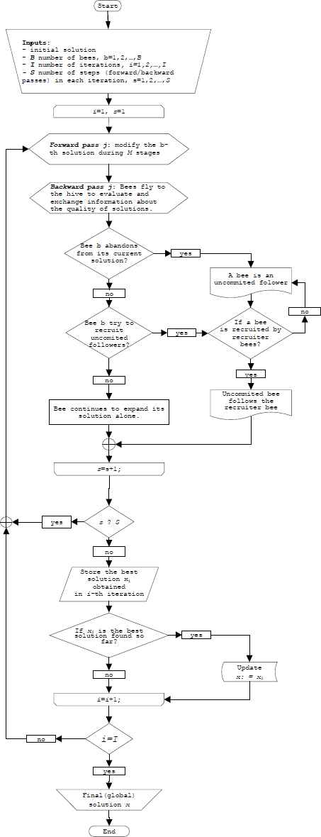
The flowchart of the BCO algorithm

4. BCOi Implementation for Max-Rev Problem

In this section, we present the implementation of described BCOi approach to solve the revenue maximization problem in optical WDM networks. The proposed model contains the following steps:

5. Experimental Evaluations

We evaluated the performances of the described Max-Rev BCOi framework by performing a numerous simulation experiments. The simulation parameters and the obtained numerical results are given below.

5.1. Simulation parameters

We have carried out a number of simulation experiments in four optical WDM network topologies shown by Fig.3: (a) a small network with N=8 nodes and L= 11 links together with three realistic size network topologies such as the (b) NSFNet (National Science Foundation Network) with N=14 nodes L=21 links, (c) EON (European Optical Network) with N=20 nodes and L=39 links and (d) USA network with N=40 nodes and L=58 links. Each physical link in all network topologies is assumed to be bidirectional, i.e. it consists of two fibers going in opposite directions. We assumed that same number of wavelengths |W| is available on each link in a network as well as up to P_k =3 pre-calculated shortest paths for every node pair (s,d).

Fig. 3.

Considered physical network topologies: (a) small network (N=8 nodes), (b) NSFNet, (c) EON, (d) USA network

We performed a huge number of simulation experiments, but due to limited space we present here only a part of the results, as given in Table 1. For example, in case of small network with N=8 nodes there are 50 experiments (30 experiments for 5 tested algorithms with |W|=6 different wavelengths in case of |K|=50 demands and 20 additional tests for different number of demands |K|≠50).

Network topology	Number of experiments
Small network (Fig 3a)	50 (30 for |K|=50 and 20 for |K|≠50)
NSFNet	50 (30 for |K|=100 and 20 for |K|≠100)
EON	60 (40 for |K|=300 and 20 for |K|≠300)
USA	84 (30 for |K|=100 and 54 for |K|=500)
	∑=244 experiments

Table 1.

The number of simulation experiments

In all simulation experiments, we used the traffic model with uniformly distributed lightpath demands between end nodes. The start time and end time of each lightpath demand are randomly generated following the uniform distribution during the planning horizon. We assumed in all simulations the planning horizon of one day with unit time slot of ΔT=1h. The revenue per a unit time slot ΔT, expressed in monetary units (m.u.) is assumed to be time dependent, as shows the Table 2.

Period of a day [h]	00-08	08-12	12-16	16-20	20-24
Revenue per time slot (ΔT), rd [m.u.]	10	20	30	20	10

Table 2.

Revenue values per time slots

Further, we assumed the following input parameters of the BCOi algorithm: number of engaged bees is set to B=10 (only in few experiments we used the set of B=20 bees to test the algorithm’s run time), number of steps (forward and backward passes) is set to be S=40 and the total number of iterations is set to I=10. To perform simulations, the programming code implemented in MATLAB language is developed. All simulation tests have been conducted using the PC equipped with Intel(R) Core(TM) 2.4GHz processor and installed (RAM) memory of 3GB.

5.2. Numerical results

To evaluate the solution quality of our BCOi Max-Rev algorithm, we compared it with other approaches, such as the heuristics Max-Profit and FCFS². Further, we compare the BCOi approach with the constructive BCO algorithm previously proposed in Ref. 9. Additionally, the BCOi approach is also compared with the optimal solution obtained by solving the ILP formulation given by Eqs. (2)–(7). Since the solution of ILP formulation is able to obtain only for small size problems, we solved it only for the small network topology with N=8 nodes, shown by Fig 3.a. The summarized comparison results for this network topology are shown by Fig.4.

Fig. 4.

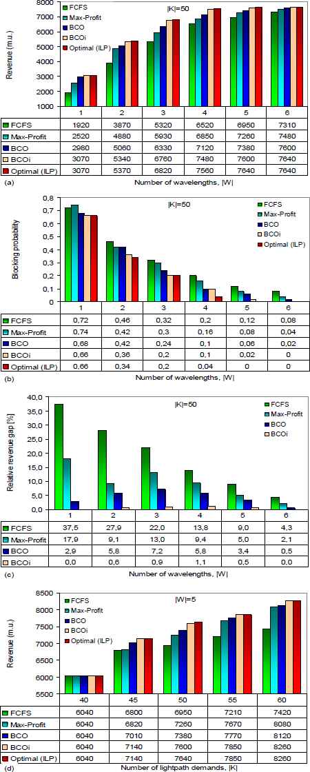
Performance comparison for small network topology (N=8): (a) revenue vs. number of wavelengths, (b) number of rejected demands, (c) relative revenue gap, (d) revenue vs. number of demands

The objective function value (i.e. total NOs revenues) as well as the number of established (rejected) lightpath demands highly depends on the number of available wavelengths in a network. It could be noticed from Fig. 4.a that our BCOi algorithm is able to produce solutions that always outperform Max-Profit, FCFS and constructive BCO algorithms according to the objective function value. We found that the minimal required number of wavelengths to establish all (|K|=50) lightpaths demands using the BCOi is |W|=6, that is the same as optimal (ILP) solution. The objective function value for BCOi and optimal solutions are the same in case of |W|=1, too. The blocking probability for considered algorithms is shown in Fig 4.b. The relative gap between obtained solutions is illustrated by graph given in Fig. 4.c. It shows in what percentage the solution obtained by any algorithm is worse than optimal (ILP) solution. As it could be seen, the BCOi approach just slightly (between 0% and 1.1%) deviates from optimal solution, while other considered algorithms have significantly greater deviations from optimal solution. The FCFS heuristic produces the worst results due to fact that in this case we have no information about profit value of demands as in the case of Max-profit. Fig 4.d shows the total revenue value obtained for different number of lightpaths demands in given network. The optimal (ILP) solution for this network example could be found only for a small number of demands (for |K|≤60).

We have also tested our BCOi algorithm in three realistic size optical networks (NSFNet, EON and USA) with various number of lightpath demands. Figure 5 illustrates the obtained results in the case of NSFNet topology. For this network example, we are not anymore able to find the optimal (ILP) solution, but only the upper bound (UB) values of the LP-relaxation problem, with a reasonable number of lightpath demands (|K|=100). Since the UB values are obtained by relaxation the integer constraints (6) and (7) of ILP model, the resulted solutions are not feasible. In such case, our BCOi model is the only approach that is able to find the feasible solutions of high quality. Once again, the revenue values obtained by our BCOi approach are of superior quality (see Fig 5.a). It could be noticed (from Fig 5.c) that BCOi solution could be better up to 3.5% compared to the constructive BCO algorithm. The BCOi solution quality improvements could be significantly higher (up to 16,2 % and 37,9%) compared to the Max-Profit and FCFS heuristics, respectively. The comparison results in the case of EON network topology are given by Fig. 6. For this network topology, it is not possible to obtain even UB values (except for small number of wavelengths, such as for |W|≤4) with a realistic number of lightpath demands (|K|=300). Fig 6.a shows the reached revenue values of the considered algorithms (for the UB solutions that could not be found, like in the cases of |W|>4, a zero value is assigned). The relative solution gap between BCOi approach and other considered algorithms is shown by Fig 6.c. It could be noticed that in this network topology BCOi approach is able to improve the solution quality even up to 5% compared to the constructive BCO approach. In order to test the possibility of BCOi algorithm to tackle with highly complex problems, we simulated it in the case of greater number of lightpath demands (up to |K|=1000). It has been shown that our BCOi approach is able to find high quality solutions within reasonable CPU times, even in case of such complex problems. The obtained revenue values are compared by Fig. 6.d. As it could be noticed, the BCOi algorithm always outperforms the considered Max-Profit, FCFS and constructive BCO algorithms.

Fig. 5.

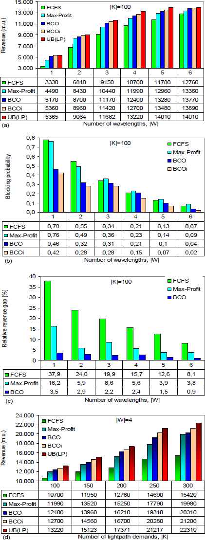
Performance comparison for NSFNet topology: (a) revenue vs. number of wavelengths, (b) number of rejected demands, (c) relative revenue gap, (d) revenue vs. number of demands

Fig. 6.

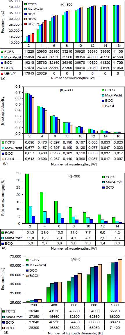
Performance comparison for EON topology: (a) revenue vs. number of wavelengths, (b) number of rejected demands, (c) relative revenue gap, (d) revenue vs. number of demands

Finally, we compare our BCOi approach to DE metaheuristic by performing simulation experiments in a more complex network topology, such as the USA network given by Fig 3.d. The control parameters of DE, the mutation constant (M) and the recombination constant (RC) are defined by the user from the range [0,1]. As suggested in Refs.17–18 for this network topology, we used the following values of the mutation and the recombination constants: M=0.2 and RC=0.5, respectively. To make more fair comparison with our BCOi approach, we have used the number of individuals in DE population of NP=10 and NP=20, the same as the number of bees in BCOi algorithm. We have carried out the simulations in this network topology for two traffic scenarios: a) case of light traffic load with |K|=100 node pair demands and b) case of moderate-to-high traffic load with |K|=500 lightpath demands. Fig. 7 and Fig. 8 illustrate the comparison results for two considered traffic scenarios in USA network topology, respectively.

Fig. 7.

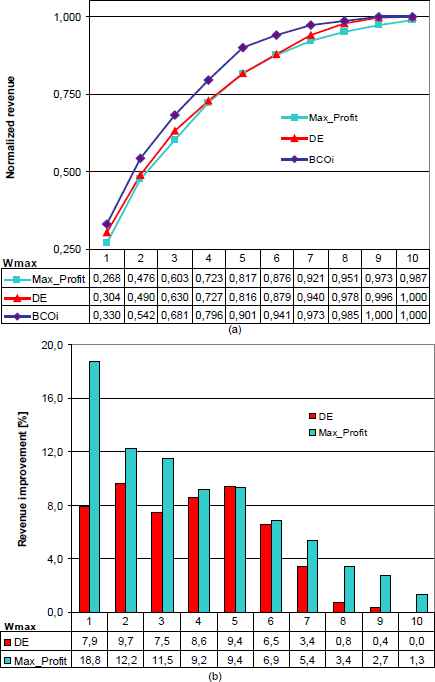
Performance comparison for USA network topology with |K|=100 demands: a) normalized revenue, b) BCOi revenue improvement relative to DE and Max-Profit algorithm

Fig.8.

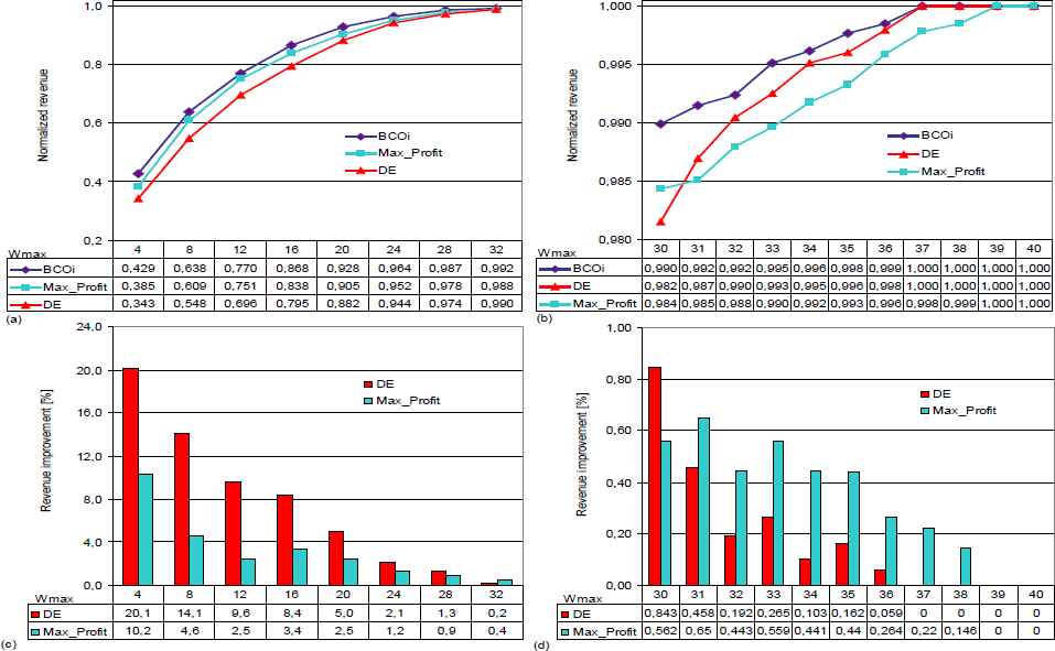
Performance comparison for USA network topology with |K|=500 traffic demands: a) Normalized revenue value for scarce number of wavelengths, b) Normalized revenue value for more appropriate number of wavelengths, c) revenue improvement relative to DE and Max-Profit algorithm in the case of scarce number of wavelengths and d) revenue improvement relative to DE and Max-Profit algorithm in the case of more appropriate number of wavelengths.

Fig 7.a shows the comparison results of the reached revenue values with BCOi, DE and Max-Profit algorithms for different number of available wavelengths (W_max). The values are normalized to the maximal potential revenue value (i.e. the revenue that could be achieved if all the requested lightpaths could be established). It could be noticed that our BCOi algorithm almost always (for different values of W_max) outperforms DE as well as Max-Profit algorithms. At the same time, DE produces revenues that are just slightly better than the Max-Profit heuristic. We can also see that for maximal normalized revenue value (1.0), the BCOi algorithm requires W_max=9 wavelengths, while DE requires one more wavelength to provide the same revenue. Fig. 7.b shows the revenue improvement that could be achieved by our BCOi algorithm compared to DE and Max-profit algorithms. Similar results are obtained in the case of moderate-tolarge traffic scenario with |K|=500 demands (Fig. 8). However, to better perceive the performances of the considered algorithms, we divide the results into 2 scenarios: Figures 8.a and 8.c (on the left side) show the results in the case of scarce number of wavelengths, while Figures 8.b and 8.d (on the right side) refer to the case of more appropriately chosen number of wavelengths to the given traffic demands. As it can be seen from Figures 8.a and 8.b, our BCOi algorithm is once more superior to DE as well as to Max-Prof algorithms. However, it could be also noticed from Fig 8.a that in the case of scarce available wavelengths DE produces even worse results than Max-profit heuristic. The reason behind that could be found in a large number of demands (|K|=500) and lack of useful information about the revenue values of individual lightpaths. With scarce available wavelengths and high number of demands, it is a challenge for DE to find a high quality complete RWA solution due to large possible random permutations while searching the solution space. By increasing the number of wavelengths, differences between the considered algorithms are reduced due to greater potential to establish more lightpaths (and consequently increase the revenues) even by using a simple heuristic, such as the Max-Profit algorithm. As a result, the relative revenue improvements of BCOi algorithm are also reduced with increasing the number of wavelengths (Fig.8c).

If the available number of wavelengths is well matched to the considered traffic demands (Fig 8.b and Fig. 8.d), DE performs better than Max-Profit algorithm. However, it is still of inferior quality compared to the BCOi algorithm. Although the relative revenue improvement of BCOi compared to DE and Max-Profit algorithms does not seem to be too high in this case (as it could be seen from Fig 8.d, it is usually less than 1%), the absolute revenue gain could be still important due to high maximal potential profit value (large number of lightpath demands). Based on the presented simulation results, one can notice that our BCOi algorithm always provides better objective (revenue) values compared to both, DE and Max-Profit algorithms. It proves our statement that BCOi approach is superior compared to other heuristic as well as metaheuristic algorithms.

Finally, we analyse various approaches used in this study (ILP, LP relaxation, BCO and DE) according to the CPU times required to find the solution. Table 3 shows the summarised results for typical simulated scenarios in different WDM networks. As it could be noticed, the number of binary integer variables (|K|(|P||W|+1)) and the number of constraints: inequalities (|W||L||T|+|K|) and equalities (|K|) highly increase with problem dimensionality. Hence, the ILP and even LP-relaxation approaches become computationally intractable in case of larger problem dimensionality. It could be noticed that CPU times for BCOi approach does not increased rapidly with problem dimensionality, as in the case of ILP. Hence, our approach could be efficiently used even for large problem dimensionality and at the same time, it is able to produce high quality solutions. It has been also shown that such solutions could be obtained using a small population of bees (by experience we used B=10 bees in simulation experiments). However, by increasing the number of bees, the required CPU times could increase notably, but the solution quality is not improved too much. Hence, the population of bees does not need to be too large in order to obtain a high quality solution with our BCOi approach. We also compared the required CPU times of DE approach. The total number of generations Gen in DE should be as high as possible to obtain the best solution. Usually, it is chosen to be in the range between 100 and 1000 depending on the problem dimension¹⁷. However, to reduce the CPU time, we limited the number of generations in all simulations to Gen=200. We also assumed the same number of individuals NP in DE as the number of bees B in BCOi. Although the CPU times of two approaches could not be directly compared (due to different concepts of BCOi iterations and DE generations), to make some reasonable comparison we assumed here an analogy between S steps of one BCO iteration (number of solutions modifications) and the number of generations Gen in DE. Using such an analogy, the required CPU times are compared, as shown in Table 3.

Case #	Network example	Number of variables	Number of constraints (ineq. + eq.)	CPU time [s]
				ILP	LP	BCOi (S=40, I=1)		DE (Gen = 40)
	Small network (N=8, L=11)					B=10	B=20	NP=10	NP=20
1	|K|=40; |W|=4; Pk=3;	520	2152 + 40	2.4	1,4	2,6	4,6	14	27
2	|K|=50; |W|=5; Pk=3;	800	2690 + 50	7,6	1,9	4,3	7,8	18	35
3	|K|=60; |W|=6; Pk=3;	1140	3228 + 60	17,9	3,8	4,5	7,5	23	45
	NSFNet (N=14, L=21)
4	|K|=100; |W|=4; Pk=3;	1300	4132 + 100	> 7200	29	11	20	47	95
5	|K|=200; |W|=8; Pk=3;	5000	8264 + 200	*	324	26	50	93	184
6	|K|=300; |W|=8; Pk=3;	7500	8364 + 300	*	685	56	113	142	553
	EON (N=20, L=39)
7	|K|=200; |W|=4; Pk=3;	2600	7688 + 200	*	197	21	41	69	136
8	|K|=600; |W|=8; Pk=3;	15000	15576 + 600	*	*	110	216	270	524
9	|K|=1000; |W|=12; Pk=3;	37000	23464 + 1000	*	*	256	519	546	1125
	USA (N=40, L=58)
10	|K|=100; |W|=10; Pk=3;	3100	14020 + 100	*	*	15	30	76	153
11	|K|=500; |W|=40; Pk=3;	60500	56180 + 500	*	*	210	417	1012	2008

*

Out of memory

Table 3.

Number of variables, constraints and required CPU times for different algorithms in considered WDM networks

6. Conclusion

In this paper, we have demonstrated the lightpaths provisioning procedure over optical WDM networks under static traffic demands, where the call admission control, routing and wavelength assignment of lightpaths is based on revenue maximization from the point of view of network operators. An optimization model based on BCOi metaheuristic has been developed to solve the Max-Rev problem. We tested our approach by performing a number of simulation experiments in different WDM network topologies. It has been proved that our BCOi Max-Rev model is able to produce near optimal solutions, which significantly outperforms some other heuristic and metaheuristic algorithms. The main advantage of the proposed model is that it is able to find high quality solutions within reasonable computational (CPU) time even in case of high complex problems. Simulation experiments show that the quality of solutions does not depend too much on the number of bees in population. It has been also shown that our BCOi model does not require “well” initial solution in order to find a high quality final solution. Altogether, superior solution qualities jointly with high efficiency of the proposed BCOi algorithm confirm that it is absolutely indispensable for NOs to maximize their revenues while establishing the lightpaths over realistic optical WDM networks.

Acknowledgements

This study is supported by the Serbian Ministry of Education, Science and Technological Development under the research grant TR32025.