
A Combination of Models for Financial Crisis Prediction: Integrating Probabilistic Neural Network with Back-Propagation based on Adaptive Boosting
- DOI
- 10.2991/ijcis.2017.10.1.35How to use a DOI?
- Keywords
- Financial Crisis Prediction; Probabilistic Neural Network; Back-Propagation; Adaptive Boosting
- Abstract
It is very important to enhance the accuracy of financial crisis prediction (FCP). Because the traditional probabilistic neural network (PNN) has some deficiencies, such as the difficult estimation of parameters and the high computational complexity, this paper proposes a new combination model, which combines back-propagation (BP) with PNN on the basis of adaptive boosting algorithm, to predict financial crisis. The BP algorithm is introduced to modify weights and smoothing parameters of PNN. In process of constructing BP-PNN models, the training set is divided into study and training samples to save the computational time. And the trained models are regarded as weak classifiers. Then these weak classifiers are integrated to constitute a stronger classifier by adaboost algorithm. To verify the superiority of the new model in terms of FCP, this article uses financial data of Chinese listed companies from Shenzhen and Shanghai Stock Exchange, and compares with adaboost BP, PNN and support vector machine models. The result shows that the new model has the highest prediction accuracy. Therefore, the new combination model is an excellent method to predict financial crisis.
- Copyright
- © 2017, the Authors. Published by Atlantis Press.
- Open Access
- This is an open access article under the CC BY-NC license (http://creativecommons.org/licences/by-nc/4.0/).
1. Introduction
The company will face a dangerous state when it suffers from financial crisis. The financial crisis includes low liquidity, inability to pay debts or dividend, substantial and continual reduction in profitability and many other aspects of financial information. The serious financial crisis brings managers, employees, investors and government to heavy financial loss. Therefore, financial crisis prediction (FCP) has important meaning for enterprise risk management. FCP is to predict whether one firm will encounter financial crisis based on the current financial condition by mathematics theory, statistical method or intelligent models.
The task of FCP mainly belongs to one kind of binary classification problem, which is to distinguish healthy firms from crisis firms. For the model, the prediction accuracy is an important factor reflecting model validity in real-world life. One model possesses the practical application value only if it has good enough prediction accuracy. Therefore, it is the main problem on FCP that how to enhance the prediction accuracy of models. Beaver was the first scholar who used a univariate model to predict enterprises bankruptcy1. Altman attempted to use multiple discriminant analysis (MDA) method to constitute the Z-score model to predict business failure2. Balcaen and Ooghe summarized and contrasted the classical statistical methodologies in business failure field3. These techniques included univariate analysis, MDA, risk index models and conditional probability models. Ohlson used the logistic model for FCP4. Zavgren used factor analysis to acquire the input variables on the basis of this research method5. But these models require data to content strict hypothesis condition, which are unsuitable to financial data.
With the development of artificial intelligence techniques, the artificial neural network (ANN) has been widely applied to FCP. Odom and Sharda applied ANN to predict business failure and compared with the MDA model6. Becerra et al. forecasted business failure of British companies by wavelet neural network models7. Li et al. used the improved back-propagation neural network (BPNN) to predict financial crisis8. Support vector machine (SVM) is a new intelligence method which can obtain ideal results in the terms of FCP9–12. There are other prediction methods, such as fuzzy sets, rough sets, genetic algorithms and so on. Chaudhuri and De employed fuzzy support vector machine for bankruptcy prediction problem13. Trabelsi et al. made classification based on rough sets14. Acosta-Gonzalez et al. employed genetic algorithms to forecast the firm failure for the Spanish building industry15. Moreover, the ensemble method could effectively enhance the prediction accuracy16. Sun and Li attempted to employ combination of multiple classifiers to predict business failure17. They used the data of Chinese listed companies to test this model and acquired the conclusion that combination of multiple classifiers had better prediction results than the single classifiers. Nanni and Lumini compared the performance of ensemble classifiers with other models in terms of bankruptcy prediction18. It is the conclusion that the ensemble system performed better. Tsai et al. made a comprehensive research about the ensemble classifier19. They respectively integrated multilayer perceptron neural networks, SVM, and decision trees based on bagging and boosting algorithm. The real-world datasets of Taiwan bankruptcy companies was used to make an experiment and obtained good performance. Therefore, it is very clear that combination models have good prediction ability.
As an excellent classifier, the probabilistic neural network (PNN) is applied to the domain of prediction20. Wang et al. employed traditional PNN model and BP neural network model for FCP21. Ticknor proposed a Bayesian regularized artificial neural network to test financial market situation22. Khashei et al. combined autoregressive integrated moving average (ARIMA) with probabilistic neural networks (PNNs) to obtain higher accuracy than traditional ARIMA models23. Adaptive boosting (AdaBoost) is generally regarded as one efficient integrated algorithm. Zhou employed the Adaboost algorithm to constitute the ensemble model to predict financial distress for Chinese listed companies24. Heo and Yang certified that AdaBoost method could obtain more excellent accuracy for the financial risk prediction of Korean construction companies25. Nie et al. presented a probability estimation model based on AdaBoost algorithm26. Zhou solved the problem of multiclass classification for Chinese listed companies by Adaboost method27.
Although the PNN model is widely applied, the deficiency still exists, such as the difficult estimate of parameters, the high computational complexity, etc. In addition, the combination of prediction models can greatly enhance the classification accuracy. Therefore, the present paper puts forward to a new combination of prediction models for FCP, which integrates back-propagation with PNN (BP-PNN) on the basis of AdaBoost algorithm. First, this paper uses back-propagation algorithm to improve classical PNN model, which can adjust weights and parameters of PNN and enhance prediction accuracy. What’s more, it is creatively mentioned that the training sample set are, during the training process, divided into study and training samples in order to reduce space complexity and computational time. Then, BP-PNN models are regarded as weak classifiers. The stronger classifier is made up of these weak classifiers by the AdaBoost algorithm. In the experiment section, this paper uses the financial data of listed companied in China and makes a comparison with the traditional prediction models to testify the superiority of this proposed model. It is the conclusion that the proposed model has the best performance. The paper is organized as follows: Section 2 introduces classical PNN. Section 3 improves the PNN with back-propagation, integrates BP-PNN models by Adaboost algorithm, and discusses the advantage of the combination model. Section 4 does empirical study and makes comparative analysis. Conclusion is provided in Section 5.
2. PNN Model
ANN is one operational model that is constituted by plenty of interconnected nodes. Every node stands for a specific activation function, and every two nodes are connected by weighted method. The different type of ANN mainly depends on different connection methods, different weight values and different activation functions. ANN includes the perceptron neural network, the BP neural network and so on. Among them, the PNN model is one classical ANN model. It is one multilayer neural network in which every layer could be respectively operated in parallel. But the PNN model is different from the universal ANN model. It has the structure of four layers and adopts activation functions which derive from statistical approach instead of general S-type activation functions. Hence, the Bayesian classification and Parzen window theorem are the basic method for this model. One example is to explain the Bayesian classification theorem. For one classification problem, x(m) = [x1,x2,…,xn] (m is number of samples, n is spatial dimension) are input vectors, which belong to several different classes (1,2,…,k). The prior probability that a sample belongs to the kth class is hk, and the cost that a sample is misclassified is ck, and the probability density function is fk(x). Bayesian classification theorem is expressed as follows:
So the sample should belong to the ith class. But it is the hardest problem to find the corresponding probability density function fk(x). The Parzen window method attempts to solve this problem. This method uses a supervised training set to estimate probability density functions. Gaussian function is often used. So probability density function is expressed as follows:
PNN model is a four-layer neural network which includes input layer, pattern layer, summation layer and output layer. The concrete network architecture is shown in Fig. 1.
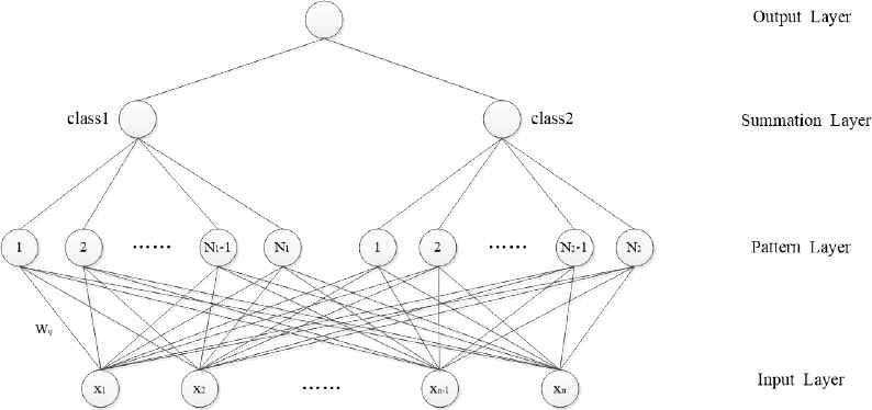
Architecture of PNN contained two classes
Because FCP belongs to one kind of binary classification problem, this article presents two classes in the network architecture. In the input layer, n nodes express one input vector with n-dimensionality, which are fully connected with nodes in the next layer. In the pattern layer, one node represents one training sample and all nodes are segmented into two classes. Every node and the input vector are calculated by probability density function to obtain the activation of each node. In the summation layer, two nodes respectively accumulate outputs of nodes of the previous layer in the same class. The node which has the bigger output value is passed to the next layer. In the output layer, there is one neuron that outputs discrete value 1 or -1 (or 0) representing the classification result.
PNN has many excellent performances, such as rapid convergence, easy training, stable neuron number and so on. This model has been widely applied to non-linear filter, pattern recognition and probability density estimation. But there are many disadvantages in this model, such as the difficult estimate of parameters and the high computational complexity. FCP uses financial indicators to predict economic conditions of one firm. The financial indicators are one kind of high-dimensional and complicated data. PNN is difficult to deal with financial indicators directly. Hence, PNN should be improved to obtain adjustable parameters and reduce space complexity and computational time.
3. The Proposed Combination Model
To solve PNN shortages, the present paper integrates BP algorithm with PNN model. To enhance prediction accuracy, the AdaBoost algorithm is adopted to integrate the improved model. First, this section introduces how to improve the PNN model with BP algorithm. Then, it illustrates the BP-PNN model on the basis of the AdaBoost algorithm. Finally, it lays emphasis on the advantage of the combination model.
3.1. Improving PNN model with BP algorithm
The BP neural network has two stages which are feed forward of input and back propagation of errors28. Based on the idea of back propagation, this article proposes one model combining back-propagation algorithm and PNN model, which is named as back-propagation + probabilistic neural network (BP-PNN). In the feed forward stage, PNN model is employed to calculate input data. In the back propagation stage, the error between the actual and desired output is transmitted from the last layer to the first layer in order to update weights and smoothing parameters. The concrete network architecture of BP-PNN model is showed in Fig. 2.
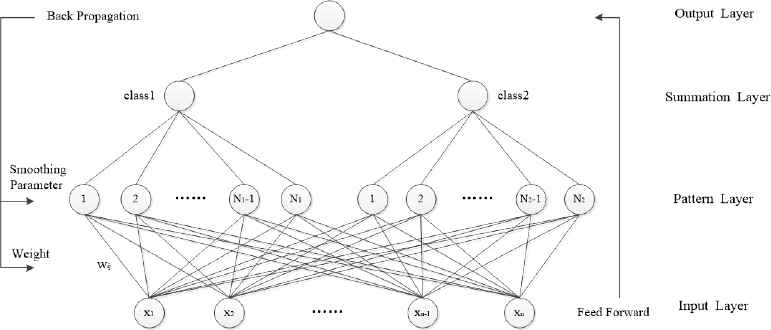
BP-PNN Architecture
where the node number of pattern layer is N (N = N1 + N2).
As shown in the Eq.(2), we can acquire probability density function fj(X)(∀j = 1,2,…, N) of the jth node in the pattern layer. F = [f1(X), f2(X),…, fj(X),… fN(X)] represents one vector which is constituted by all of probability density functions in the pattern layer. D is one N × 2 matrix that means to which class node of the summation layer nodes of the pattern layer should belong. DN×2 = [dij](∀i = 1,2,…, N ; ∀j = 1,2). The expression of classification vector S in the summation layer is shown as follows:
The error value is between 0 and 1. When
- (1)
The weight modification
As the PNN model, wij expresses one weight between the ith node in the input layer and the jth node in the pattern layer. The concrete expression is shown as follows:
where xi represents the ith variable of an input vector. Therefore, X and Xj in the Eq.(2) should be separately expressed as follows:where xi is the ith variable of n-dimensional input vector,where β is the learning rate value. As the jth element in F, we can obtain the update expression of weights based on Eq.(1) as follows:Therefore, we can obtain the following vector.
Then, it is easy to obtain the final update weight by putting Eq.(11) and (12) to Eq.(10).
- (2)
The smoothing parameter modification
Similarly, we can build the update expression of smoothing parameters.
Therefore, as the jth node of the pattern layer, the specific update expression is shown as follows:
We can obtain the following vector.
The parameter modification of BP-PNN model has been completed. It is another important problem to reduce space complexity and computational time. As the same as the PNN model, the fewer nodes the pattern layer has, the less time this new model spends. However, the number of nodes in the pattern layer equals the number of samples in the training set. In another words, if one training set has fewer samples, this model can save more time. Because of the introduction of BP algorithm, this model needs not to be trained by all of training samples. Hence, this article divides the training set into study and training samples. The study samples are used to confirm the node number of the pattern layer and initial weights in order to create the original PNN model. The training samples are adopted to revise weight value and smoothing parameter by the back-propagation algorithm above. Therefore, it can save the computational time that the training set is divided into study and training samples. It is means that the ratio between study and training samples affects the computational time directly. It is easy to make poor performance for this model if the ratio is too low, whereas the computational time can’t be saved and this method loses practical significance. This paper select the 3:7 ratio to distribute study and training samples. The reason is that such ratio can not only conform to the training characteristic of BP algorithm, but meet the selection rule for two classes of samples in extensive studies. In the empirical study, the comparison of different ratio is provided to testify the superiority of this ratio.
The concrete process is that, first, the training set are classified according to healthy and unhealthy companies. Then, 30% of data are randomly selected from every classification to be study samples, and the others are training samples. This process can help the balance of every category for study and training samples.
3.2. The AdaBoost Algorithm with BP-PNN
AdaBoost algorithm is derived from Boosting algorithm. This algorithm can integrate some weak classifiers to construct one stronger classifier to enhance prediction accuracy. Its adaptivity can be shown that the samples which are misclassified by the previous weak classifier are drawn more attention, and the weighted samples are used to train the next weak classifier again. As the same time, one new weak classifier is joined every time until this model satisfies some specific conditions. The concrete realizing process is described: every input sample is assigned one equal weight. Then, if one sample is misclassified, its weight should become bigger. If not, its weight should become smaller. The samples whose weights are modified are to train next weak classifier. Last, the strong classifier is constituted by all weak classifiers.
This article proposes one new model which integrates BP-PNN models by adaBoost algorithm. The framework of the new model is shown in Fig. 3. First, the raw data are preprocessed to reduce the dimensionality and simplify the complexity of raw data. Then, the processed data are divided into training and testing set by cross validation method to increase the number of samples. Next, the training set is separated into study and training samples to train the BP-PNN weak classifier. The weight of weak classifier is calculated according to the error rate after the completion of the training. Besides, the weights of the data are updated. If one sample is misclassified, its weight is increased, and the next weak classifier pays more attention to this sample; otherwise, its weight is decreased. After all BP-PNN weak classifiers finish the training, the stronger classifier is constructed. Finally, the testing set is calculated by the stronger classifier to obtain the prediction result.
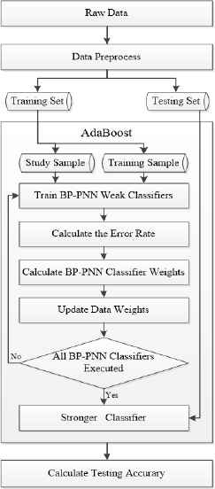
Framework of the Proposed Model.
The concrete calculation process of the proposed model can be summarized as follows:
Step 1: The training set S = {(X1,Y1),…,(Xi,Yi),…,(Xn,Yn)} is given, where X represents an input vector and Y is a (0 or 1) vector expressing classification results.
Step 2: The weights of training samples are initialized as D1(i) = 1/n.
Step 3: The max iteration time is set as T, t = 1,2,…,T.
Step 3.1: The model is trained by the study and training samples with weights Dt to construct a BP-PNN classifier ht, its classification outputs are ht = {ht(1),ht(2),…,ht(n)}.
Step 3.2: According to prediction results, the total error is calculated,
Step 3.3: The iteration can’t be stopped until et is enough small.
Step 3.4: Calculate weight of the BP-PNN weak classifier ht,
Step 3.5: The weight Dt can be updated as follows:
Step 4: The stronger classifier is obtained,
Then, the final result is one positive number, this sample belongs to one classification. Inversely, this sample belongs to another classification.
3.3. The Advantage of the Combination Model
The proposed model considers BP-PNN as a weak classifier and uses adaboost algorithm to build a stronger classifier, which combines the advantage of the PNN model, BP and adaboost algorithm.
The BP-PNN model combines the feature of the PNN and BP algorithm: The PNN model can deal with deficiency or noise data set, decide to the model structure, and easily confirm the node number of the middle layer, which solve problems for the BP algorithm. The BP algorithm can modify the parameters and weight values, which can overcome simplex learning-method of the PNN model and enhance the accuracy. In addition, the method that the training set is divided into study and training samples can save the computational time.
The adaBoost algorithm demands that the accuracy of weak classifiers are merely better than estimation value, which may further save computational time by reducing the training iterations. The accuracy can be obviously enhanced because of the advantage of the adaBoost algorithm.
In addition, the over-fitting problem widely exists in the intelligence algorithm. But this proposed model can’t be troubled in this problem. There are three reasons that, first, the data can be reduced the dimensionality by preprocessing to simplify the complexity of data, which can’t result in a complicated classifier for dealing with the data. Second, this model adopts cross validation to increase the number of trained samples, which can prohibit the over-fitting situation that too few samples induce. Third, as the weak classifier, the BP-PNN is one optimization model with the simple structure. And many optimization models are integrated by adaboost algorithm, which can’t create the over-fitting situation to which one singular sample or one weak classifier lead.
4. Empirical study
4.1. Selection of sample companies and financial indicators
If Chinese listed companies had negative net profit in two consecutive years or deliberately announced the false financial condition, they would be specially treated by China Securities Supervision and Management Committee (CSSMC). And ST is added to the front of such companies’ names in the stock exchange. According to the principle of the same time, the same industry and the similar capital scale, 200 samples, which are the manufacture industry, are selected from Shenzhen and Shanghai Stock Exchange from 2010 to 2012. These samples contain 100 normal companies and 100 ST firms.
The selection of financial indicators need not only directly reflect the financial situation, but also consider the dimensionality of sample data. Hence, 20 financial indicators are selected, which are showed in Table 1. Some financial indicators have mutual effect to reflect one aspect of financial situation. As shown in Table 1, these financial indicators reflect 4 important aspects which are activity ability, solvency, profitability and growth ratio.
| Category | Variables | Definition |
|---|---|---|
| Activity Ability | X1 | Inventory turnover ratio |
| X2 | Receivables turnover ratio | |
| X3 | Current assets turnover | |
| X4 | Fixed assets turnover | |
| X5 | Total assets turnover | |
| Solvency | X6 | Current ratio |
| X7 | Quick ratio | |
| X8 | Debt to total assets ratio | |
| X9 | Cash flow to current liability | |
| Profitability | X10 | Net assets income rate |
| X11 | Return on assets ratio | |
| X12 | Net capital income rate | |
| X13 | Net profit margin of sales | |
| X14 | Earnings per share | |
| Growth ratio | X15 | Growth ratio of income per share |
| X16 | Growth ratio of total assets | |
| X17 | Growth ratio of operating income | |
| X18 | Growth ratio of operating profit | |
| X19 | Growth ratio of total profit | |
| X20 | Growth ratio of net profit | |
Financial Indicators’ Definition and Category
4.2. The preprocessing of financial data
Although such financial indicators can accurately reflect financial situation, so many variables increase computational time and easily obtain poor performance. Furthermore, there are strong or weak correlations among these indicators, which increase the probability of repeated information and make many unnecessary troubles. We use factor analysis method to solve these problems. Factor analysis method can use a few comprehensive variables to stand for original data variables based on the loss of the least information. These comprehensive variables are named as common factors. Therefore, we adopt the factor analysis to reduce the complexity of the calculation and enhance the accuracy.
In this paper, we use software SPSS 19.0 to run factor analysis method to obtain common factors from 20 financial indicators of 200 samples. First, the correlations among these indicators are examined by KMO and Bartlett’s test in order to determine whether the data were appropriate for factor analysis. As shown in Table 2, the value of KMO is 0.691, which is bigger than 0.5. It means that partial correlations are enough strong for these indicators. For Bartlett’s test of sphericity, the value of Sig. is 0.000 (<0.05), which signifies that strong correlations exist among these indicators. Therefore, these sample data are suitable for factor analysis.
| Kaiser-Meyer-Olkin | Measure of Sampling Adequacy. | .691 |
|---|---|---|
| Bartlett’s Test of | Approx. Chi-Square | 5067. |
| Sphericity | 647 | |
| df | 190 | |
| Sig. | .000 |
KMO and Bartlett’s Test
Next, total variance explained is obtained in Table 3. 5 factors’ eigenvalues are greater than 1, and the cumulative rate of contribution is 82.838%, which is more than 80%. Therefore, 5 common factors are selected, which contain most of the main financial information.
| Component | Initial Eigenvalues | Extraction Sums of Squared Loadings | Rotation Sums of Squared Loadings | ||||||
|---|---|---|---|---|---|---|---|---|---|
| Total | % of Variance | Cumulative % | Total | % of Variance | Cumulative % | Total | % of Variance | Cumulative % | |
| 1 | 7.052 | 35.258 | 35.258 | 7.052 | 35.258 | 35.258 | 5.787 | 28.934 | 28.934 |
| 2 | 3.375 | 16.874 | 52.132 | 3.375 | 16.874 | 52.132 | 3.020 | 15.099 | 44.033 |
| 3 | 2.535 | 12.677 | 64.809 | 2.535 | 12.677 | 64.809 | 2.997 | 14.987 | 59.021 |
| 4 | 1.863 | 9.317 | 74.126 | 1.863 | 9.317 | 74.126 | 2.506 | 12.529 | 71.550 |
| 5 | 1.742 | 8.711 | 82.838 | 1.742 | 8.711 | 82.838 | 2.258 | 11.288 | 82.838 |
| 6 | .899 | 4.496 | 87.333 | ||||||
Total Variance Explained
5 common factors respectively include different financial indicators. The first common factor F1 represents profitability which is explained by X10, X11, X12, X13, X14. The second common factor F2 represents growth ability which is explained by X15, X16, X17, X18, X19, X20. The third common factor F3 represents long-term activity ability which is explained by X1, X4. The fourth common factor F4 represents repay debt ability which is explained by X6, X7, X8, X9. The fifth common factor F5 represents short-term activity ability which is explained by X2, X3, X5. These 5 common factors are regarded as input variables of the model.
4.3. Experiment design
This article adopts the 10-folds cross validation to construct training set and testing set. First, normal and ST companies are averagely divided into 10 portions respectively. The random 5 portions are selected as training set and the others are testing set, which can guarantee that the training set has 50 normal companies and 50 ST firms, and testing set includes 50 normal companies and 50 ST firms. Then, during the training process, normal and ST companies, respectively, are divided into study and training samples according to the 3:7 ratio. Besides, 10 weak classifiers are used to construct prediction model, and every model adopts 100 iterations or one standard, that the gradient of an trained parameter is less than 1‰, to gradually modify weights and smoothing parameters.
The 2:8 and 4:6 ratios between study and training samples are made comparative analysis in order to verify the performance of the 3:7 ratio. In addition, because the new model is on the basis of BP-PNN and adaBoost algorithm, adaBoost BP, PNN and SVM are selected as contrast models. All of models are implemented in the MATLAB R2012b package software.
4.4. Result and comparison
4.4.1. Results on Ada BP-PNN model
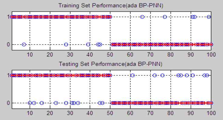
This article distributes study and training samples according to the 3:7 ratio. To testify the superiority of such ratio, another two kinds of ratios, which are 2:8 and 4:6 ratios, are made comparison analysis. All of the prediction performances are shown in the Fig. 4–6, which express results of 2:8 ratio, 3:7 ratio and 4:6 ratio in sequence. The X-axis represents the number of sample companies, and Y-axis represents classification result. Y-axis contains two values that are 1 and 0, which respectively stand for healthy companies and ST companies. In figures, the red asterisk (*) stands for the classification of sample companies in fact, and the blue round (o) expresses prediction results. The sample company is correctly classified if two signs coincide. Otherwise, it is misclassified.
Performance of Ada BP-PNN Model According to the 2:8 Ratio
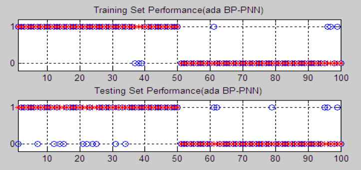
Performance of Ada BP-PNN Model of the 3:7 Ratio
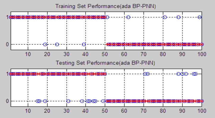
Performance of Ada BP-PNN Model of the 4:6 Ratio
The detailed results of prediction performances and computational time are listed in the Table 4. For the 2:8 ratio, 45 normal companies and 45 ST companies are correctly classified during the training stage. It has the total accuracy of 90%. In the testing stage, 40 companies and 41 ST companies are correctly classified and the total accuracy is 81%. The averaged running time is 13.973s. For the 3:7 ratio, 47 normal companies and 46 ST companies in the training set are correctly classified, and 39 normal companies and 44 ST companies in the testing set are correctly classified. The total accuracy of training and testing, respectively, are 93% and 83%. It spends 15.073s on averaged computational time. For the 4:6 ratio, 47 normal companies and 46 ST companies are correctly predicted during the training stage, and 40 normal companies and 43 ST companies are correctly predicted for the testing set. 92% and 83% are the total accuracies of training set and testing set respectively. The averaged running time is 25.486s.
| Ratio | Description | Training Set | Testing Set | Averaged Time | ||||
|---|---|---|---|---|---|---|---|---|
| Quantity | Accurate number | Quantity | Accurate number | |||||
| 2:8 | Normal Companies | 50 | 45 | 50 | 40 | 13.973s | ||
| ST Companies | 50 | 45 | 50 | 41 | ||||
| Accuracy | 90% | 81% | ||||||
| 3:7 | Normal Companies | 50 | 47 | 50 | 39 | 15.073s | ||
| ST Companies | 50 | 46 | 50 | 44 | ||||
| Accuracy | 93% | 83% | ||||||
| 4:6 | Normal Companies | 50 | 47 | 50 | 40 | 25.486s | ||
| ST Companies | 50 | 45 | 50 | 43 | ||||
| Accuracy | 92% | 83% | ||||||
Prediction Performance of Ada BP-PNN Model
From the prediction results of different ratios, although the 3:7 ratio needs a litter more time than the 2:8 ratio, the 3:7 ratio has better performance. That is the reason that the node number of pattern layer should not be too few. Although there are about the same accuracies between 3:7 and 4:6 ratios, the latter needs more computational time. Therefore, the 3:7 ratio are the most suitable allocation proportion.
Besides, 18 different financial indicators are selected from 200 sample companies that are employed by this article to make comparative analysis. These indicators are preprocessed by the same method, and are calculated by the proposed model. The prediction accuracies of training and testing set are 86% and 79% respectively, which are lower than the accuracy in Table 4.
4.4.2 Comparison between Ada BP-PNN model and other classifiers
In order to testify whether the proposed model can enhance the accuracy, this section uses three classifiers, which are the Ada BP, PNN and SVM model, to make comparative analysis. Their concrete prediction performances are shown in the Fig. 7–9. Every figure contains the outcome of training set and testing set.
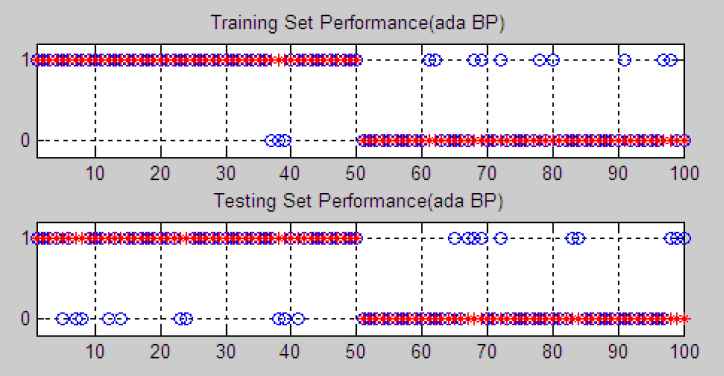
Performance of Ada BP Model
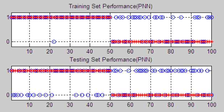
Performance of PNN Model
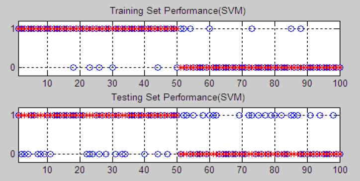
Performance of SVM Model
In this article, the ada BP model adopts back-propagation as the weak classifier, and the SVM model uses the radial basis function as the kernel function. It respectively shows the prediction performances and computational time of ada BP model, PNN model and SVM model in Table 5. It is very clear that, for the training set or testing set, the ada BP model has the greatest prediction accuracies, which are 87% and 80% respectively. The next one is SVM model, which are 87% and 71% respectively. The last one is PNN model, which are 76% and 56% respectively. Such result can testify the superiority of adaBoost algorithm. Then, to compare the data in Table 4 with Table 5, the new model proposed by this article has the best prediction accuracy than the other three models, and which is also shown in Fig. 10. Besides, three contrast models cost 15.018s, 4.080s and 12.897s respectively. The new model needs the time which approximates to the ada BP model. Although the new model needs a litter more time than PNN and SVM, it can sharply enhance prediction accuracy.
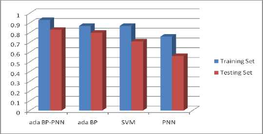
Prediction Accuracies of Models
| Model | Description | Training Set | Testing Set | Averaged Time | ||||
|---|---|---|---|---|---|---|---|---|
| Quantity | Accurate number | Quantity | Accurate number | |||||
| Ada BP | Normal Companies | 50 | 47 | 50 | 40 | 15.018s | ||
| ST Companies | 50 | 40 | 50 | 40 | ||||
| Accuracy | 87% | 80% | ||||||
| PNN | Normal Companies | 50 | 49 | 50 | 34 | 4.080s | ||
| ST Companies | 50 | 27 | 50 | 22 | ||||
| Accuracy | 76% | 56% | ||||||
| SVM | Normal Companies | 50 | 44 | 50 | 32 | 12.897s | ||
| ST Companies | 50 | 43 | 50 | 39 | ||||
| Accuracy | 87% | 71% | ||||||
Prediction Performance of Contrast Models
First, it compares prediction results of ada BP-PNN and ada BP models with the SVM and PNN. The models of adaboost algorithm, whether from the training and testing set, have better performance than the latter two models, which can demonstrate that adaboost algorithm is good at FCP. Then, it compares classification performance of ada BP-PNN with ada BP. As shown in Fig. 10, the accuracies of training and testing set from the proposed model are better than the result of the latter model. It is the reason that the new model uses the theory of back-propagation to optimize parameters of PNN. And as a weak classifier, the improved BP-PNN model is integrated by adaboost algorithm. The stronger classifier has better prediction accuracy. Therefore, it can demonstrate that ada BP-PNN model is one better classifier.
5. Conclusion
This paper proposes one new combination of prediction models for financial crisis. This model combines BP algorithm with PNN model on the basis of adaBoost algorithm. In the first section, this article employs BP algorithm to improve the structure of PNN model. It is creatively mentioned that the training set is divided into study and training samples during the training process. The study samples are used to create the BP-PNN model, and the training samples are used to modify weights and smoothing parameters for the BP-PNN model. In the next section, the BP-PNN models that are trained by randomly ranking samples are considered as weak classifiers. According to the AdaBoost algorithm, the stronger classifier is constructed by these weak classifiers. Whether companies are specially treated is the criterion that crisis companies and normal firms are distinguished. The specially treated companies are regarded as financial crisis enterprises, otherwise they are normal enterprises. To compare with other models, this new model can obtain ideal prediction outcomes. The main contributions in this paper have three aspects. First, the BP algorithm is used to improve the computation rule of PNN model, which can modify simplex learning-method for the PNN model and enhance the prediction performance. Second, since the advantages of the adaBoost algorithm, the BP-PNN on the basis of adaBoost algorithm can efficiently enhance the prediction accuracy. Third, the key point is to enhance the models’ prediction accuracy for FCP. The comparative experiment among different models has shown that this new ensemble model can more successfully predict the result whether the financial crisis will occur. Therefore, the ensemble model presented by this paper is more suitable to FCP.
Acknowledgement
The research in this paper has been supported by the National Natural Science Foundation of China under Grant No. 71271070.
References
Cite this article
TY  - JOUR
AU  - Lu Wang
AU  - Chong Wu
PY  - 2017
DA  - 2017/01/01
TI  - A Combination of Models for Financial Crisis Prediction: Integrating Probabilistic Neural Network with Back-Propagation based on Adaptive Boosting
JO  - International Journal of Computational Intelligence Systems
SP  - 507
EP  - 520
VL  - 10
IS  - 1
SN  - 1875-6883
UR  - https://doi.org/10.2991/ijcis.2017.10.1.35
DO  - 10.2991/ijcis.2017.10.1.35
ID  - Wang2017
ER  -