
Combination Replicas Placements Strategy for Data sets from Cost-effective View in the Cloud*
- DOI
- 10.2991/ijcis.10.1.521How to use a DOI?
- Keywords
- Cloud environment; Cost-effective; Replicas placements; Pseudo-replicas; Replicas
- Abstract
In the cloud storage system, data sets replicas technology can efficiently enhance data availability and thereby increase the system reliability by replicating commonly used data sets in geographically different data centers. Most current approaches largely focus on system performance improvement by placing replicas for an independent data set, omitting the generation relationship among data sets. Furthermore, cost is an important element in deciding replicas number and their stored places, which can cause great financial burden for cloud clients because the cost for replicas storage and consistency maintenance may lead to high overhead with the number of new replicas increased in a pay-as-you-go paradigm. In this paper, we propose a combination strategy of real-replicas and pseudo-replicas (by computation from its provenance) from cost-effective view in order to achieve the minimum data set management cost, not only for the independent data sets but also for related data sets with generation relationships. We first define cost models that fit into the cloud computing paradigm, including data sets storage, computation and transfer costs, and then develop a new data set management cost model, helping to achieve a multi-criteria optimization of data set management. After that, a minimum cost benchmarking approach for the best trade-off between real-replicas and pseudo-replicas is proposed once decision to add a replica has been made. Then, a more practical and reasonable genetic algorithm as an alternative procedure for generating optimal or near-optimal solution is given in order to identify the suitable replicas storage places. Finally, we present simulations setups and results that provide a first validation of our strategy. Both the theoretical analysis and simulations conducted on general (random) data sets as well as specific real world applications have shown efficiency and effectiveness of the improved system brought by the proposed strategy in cloud computing environment.
- Copyright
- © 2017, the Authors. Published by Atlantis Press.
- Open Access
- This is an open access article under the CC BY-NC license (http://creativecommons.org/licences/by-nc/4.0/).
1. Introduction
Cloud service providers, such as Amazon S3 [1], Google Cloud Storage (GCS) [2], and Microsoft Azure [3] offer storage as a service by providing storage resources in several data centers distributed around the world. Clients (users) can store and retrieve data sets without dealing with the complexities associated with setting up and managing the underlying storage infrastructures [4, 5]. On the same time, replication techniques have been commonly used to minimize the communication latency, increase fault tolerance, improve data availability and thereby increase the system reliability by bringing the data sets closer to the clients [6–9].
Nevertheless, there are still two important challenges if we applied these technologies directly to the data sets replicas management in the cloud: (1) in theory, clients can get unlimited storage resources in the cloud. However, they also have to pay for resource consumption due to cloud’s “pay-as-you-go” model. Meanwhile, replicas mean extra storage resource consumption, and the more replicas in the system, the higher storage cost will be. In this way, existence of data set replicas can improve system performance at the expense of much more storage cost, and further result in the increase of data sets management cost [11–12]. Also the number of replicas and their store placements are important questions to be solved from cost-effective view. Unfortunately, most of the existing works only focused on system performance improvement by creating/deleting replicas [6–8]. Although, some works have been studied placing replicas from cost-effective in the data grid, while these algorithms can not be directly used in the cloud storage system due to hierarchical network structure and special data access patterns [9–10]. And (2) in the cloud, each data center only hosts a subset of the whole data sets, and these data sets can generate other related data sets at the expense of computation resource consumption. In anther words, there exist generation (derivation) relationships [13–14] among data sets. Therefore, it is an intelligent way to generate a data set from its provenance immediately and then transfer it after receiving clients’ requests. That is to say, the retrieved data set is not from the real data set or its replicas but generation from its provenance, which effectively reduce data storage cost despite of increased extra computation cost. For example, there is a data set di stored on data center dcm, and di can be generated from data set dj while the application runs. In this way, if a decision to create di′ s replica di′ and store it on dck has been made, then a more intelligent approach is to first compare the storage cost of di′ and computation cost from data set dj with all else equal, then to choose the one with less data manage cost between real replica and generation data set. Hence, the better performance and lower cost can be achieved. It should be pointed out that generation relations are common among data sets in cloud environment. Although there are many works related to data sets replicas placements in the past years, relatively few approaches related to the replicas placements optimization from the cost view. And all the current solutions are based assuming that data sets are independent of each other, omitting the generation relationships among data sets.
In this paper, our research objective is to develop a minimum benchmarking approach for the best trade-off between data set’s real-replicas and pseudo-replicas (that means the replica is not a static data set stored on data center, but regenerate from its predecessors immediately if necessary) from cost-effective view. In particular, we intend to construct an overall cost model that can be used to decide the real replicas numbers and their stored places, or the provenance if pseudo-replicas needed. This cost model comprises a comprehensive set of cost factors, necessary for making reasonable cost estimation for running applications in an in-house data center or on a public cloud. To achieve this, we first perform a systematic literature review of papers on data sets replicas and cost models in cloud computing. Second, we design cost models for storing, transferring and computing over wide cloud architecture. Based on these results, we perform a cost-benefit analysis to design a comprehensive overall cost model for data management. Then, we propose a combination strategy involving real and pseudo-replicas technique, which leads to the theoretical minimum data management cost using generic algorithm (GA). Finally, we apply this combination data sets replicas strategy to demonstrate its working.
The contributions of this research include: (i) develops a data set management cost model in the cloud and show that replicas placements can be done in a distributed manner; (ii) proposes a combination data sets replicas placements strategy from cost-effective view; (iii) gives a heuristic algorithm for the combination replicas placements strategy in the widely cloud system and prove that it can stabilize and converge to optimal in a bounded time period.
2. Related works
In this section, we first introduce data sets replicas placements technology, and then describe a typical data sets management pricing model, illustrated by some of Amazon Web Services (AWS). At last, we briefly recall the data sets types in the cloud.
2.1. Data sets replicas placements technology
With the advancement and development of various technologies, data sets replicas placements in distributed systems have been studied in many works, which are referenced and adopted in cloud data set replication. Data replication algorithms can be classified into two groups: static replication [15] and dynamic replication algorithms [16–17]. In a static replication model, the replication strategy is predetermined and well defined. On the other hand, dynamic replication automatically creates and deletes replicas according to changing access patterns. Table 1 summarizes the related replicas placements technologies in recent years.
| No. | Methodology | Replication Classification | Network used | Simulator used | Evaluation Parameters | Performance |
|---|---|---|---|---|---|---|
| 1 | Branch Replication Scheme(BRS)[18] | Distributed | Tree data grid | Omnet++ | Usage, Number of intercommunications, bandwidth consumption, Response time, Network Latency | Improved data access performance than hierarchical (HRS) and server-directed (SDRS). |
| 2 | No Replication, Best Client, Cascading Replication, Plain Caching, Caching plus Cascading Replication and Fast Spread Strategy [19] | Distributed | Graph | OptorSim | Communication Cost | Reduced communication cost than K-replication, No replication and complete replication. |
| 3 | Replica Placement based on social ability [20] | Not mentioned | Free-Scale Topology | OptorSim | Storage used, Makespan | Better than Simple Replication. Always Replicate. |
| 4 | SWORD: A workload-aware data placement and replication approach [21] | Distributed | Cloud | Amazon EC2 medium instances | minimize query span and replication resource consumptio | Improves transaction latencies and overall throughput |
| 5 | Hierarchical Replication Scheme (HRS)[22] | Distributed | Hierarchical Cluster grid Structure | OptorSim and Taiwan Unigrid | Total job Execution Time, computing Resource | Total job execution time is 40% faster than BHR optimizer than LRU and LFU |
| 6 | FindR, MaxR, AffinityR and MinMaxLoad[23] | Centralized | Hierarchical Grid (Unconstrained mode, Constrained mode) | Taiwan knowledge innovation National Grid | Makespan, Tree balance, Ratio of Feasible Placement, Number of Replica Servers, Capacity of a Replica Server (CRS), Mean of Data Request Distribution on the client (MDR) | FindR and MinMaxLoad are best in terms of number of replicas and balancing the workload. MMxR and Affinity R are comparative in reducing the number of replicas and MaxR is superior to AffinityR in balancing workload. |
| 7 | Latest Access Largest Weight (LALW)[24] | Distributed | Hierarchical Architecture | Optorsim | Storage element utilization, Total number of replications, Average job time, Network utilization | Mean job execution is about 15% faster than simple Optimizer. ENU is 16% lower than LFU and also saves storage space. |
| 8 | Economy-based File Replication Strategy[25] | Distributed | Not Mentioned | OptorSim | Total job execution time | Improved performance of economic model compared to traditional replication algorithms. |
Comparison of replicas placements technologies
2.2. Data sets management pricing policies
Cloud service providers (CSPs) supply a pool of resources, such as hardware (CPU, storage, networks, etc.), development platforms and services [26] with different pricing policies. This paper relies on a limited, yet representative enough model that include the main, commonly billed elements in data sets management, i.e., CPU, storage and bandwidth consumption. In order for readers to have an overview of pricing policy, we present a simplified version of AWS offer.
The Amazon Simple Storage Service (S3) supplies storage capabilities [1]. In this model, the price varies with respect to data set size, with an earned rate when data size increase, as is shown in Table 2.
| Data set size | Price per month per GB |
|---|---|
| First 1TB | $ 0.14 |
| Next 49 TB | $ 0.125 |
| Next 450 TB | $ 0.11 |
| … | … |
Amazon storage prices
Network bandwidth consumption is billed with respect to data set volume, as illustrated in Table 3. In this model, input data sets transfers are free; whereas output data set transfer cost varies with respect to data volume, with an earned rate when volume increases. When applying this pricing model, the cost of bandwidth consumption can be acquired if storage time and data size are known.
| Data set size | Price per time |
|---|---|
| Input data set | |
| Any input data | free |
| Output data set | |
| First 1GB | free |
| Up to 10 TB | $ 0.12 per GB |
| Next 40 TB | $ 0.09 per GB |
| Next 100TB | $ 0.07 per GB |
| … | … |
Amazon bandwidth prices
Finally, In AWS, Elastic Compute Cloud (EC3) provides computing resources [1]. Different instances configurations can be rent (micro, small, large, extra large, etc.) at various prices. As illustrated in Table 4.
| Instance configuration | Price per hour |
|---|---|
| Micro | $ 0.03 |
| Small | $ 0.12 |
| Large | $ 0.48 |
| Extra large | $ 0.96 |
| … | … |
EC2 computing prices
3. Data sets cost models in the cloud
In this section, we will present data sets models used in this paper. Specifically, we first introduce some definitions related to cloud computing environment. Then, we describe data sets provenance and data dependency graph, which are used to depict the data sets generation relationships.
3.1. Cloud computing environment
Ideally, clients of cloud services do not need to worry about scalability because the resource provided is virtually infinite and the network links are virtually capable to quickly transfer any quantity of data sets between the available servers. Data centers and their connections, which provide clients with the physical infrastructures need to host their computer systems, are main components of cloud computing environment.
Definition 1.
Cloud computing environment (CCE). Cloud computing environment can be described as a pair: (DC, B), where,
- (i)
DC is a set of distributed data centers, written as
- (ii)
B is a matrix, representing bandwidth between data centers, and the element bij means the bandwidth between two data centers dci and dcj, indicating the network transmission capacity.
The bandwidth may fluctuate from time to time according to peak or off-peak data access time in practice. In this paper, we simplify the problem and regard the bandwidth as a static value, ignoring the volatility during different access time. On the other hand, the value of bandwidth means the time of transferring data from one data center to another. So, we will use the bandwidth as a basis for calculating the transfer time in the following section. Fig 1 depicts a typical architecture of a cloud computing environment with 7 data centers.
Architecture of cloud computing environment.
Data centers provide the basic ingredients such as storage, CPUs, and network bandwidth as a commodity by specialized service providers at low unit cost. In this paper, we define the data center as follows.
Definition 2.
Data center (DC). Each data center dci∈DC can be described as a 7-tuple (dci, spi, cpi, tpi, D, tsi, vsi), where,
- (i)
dci is the identifier of a data center, and is unique in CCE;
- (ii)
spi means the storage price policy of data center dci;
- (iii)
cpi means the computation price policy of data center dci;
- (iv)
tpi means the transfer price policy of data center dci. Usually, spi, cpi and tpi are all determined by the cloud service providers;
- (v)
D=Dorg⋃Dgen is a set of original data set and generated data sets on the data center dci;
- (vi)
tsi is the total space of data center dci, whose unit is TB; and,
- (vii)
vsi is the size of vacant space on data center; means the extra storage capacity of dci.
A data set involves its size, stored places and its provenance. In this paper, we define a data set as follows.
Definition 3.
Data set (D). A data set dm∈D can be described as a 5-tuple (dm, sm, sp, fi, provSetm), where,
- (i)
dm is the identifier of data set, which is unique in the cloud;
- (ii)
sm is the size of data set dm;
- (iii)
sp∈DC, is the data set dm’s storage place;
- (iv)
fi is a flag, which denotes the status whether data set dm is stored or deleted in the system; and,
- (v)
provSetm is the set of stored provenances that are needed when regenerating data set dm. The detailed description of provSetm will be given in Definition 5.
3.2. Data sets dependency graph and data set provenance
Data sets provenance is a kind of important metadata which records the dependencies among data sets, i.e. the information of how the data sets were generated. Taking advantage of data sets provenance, we can build a data sets dependency graph.
Definition 4.
Data sets dependency graph (DDG). Data sets dependency graph is a directed acyclic graph, and can be described as a 3-tuple (VD, E, φ), where,
- (i)
VD={d1, d2, …}, is a set of nodes; and each node denotes a data set;
- (ii)
E={e1, e2, …}, is a set of edges between pair of nodes;
- (iii)
φ is a mapping from each edge ek to pair of nodes (di, dj) if these two data sets, di and dj, have generation relationship, in other words, di is a predecessor data set of dj.
Fig 2 shows a simple DDG, where each node in the graph denotes a data set.
A simple data dependency graph.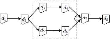
In Fig 2, data set d1 pointing to data set d2 means that d1 is used to generated d2; and d2 pointing to d3 and d5 means that d2 is used to generate d3 and d5 based on different operations. Also, data set d4 and d6 pointing to dataset d7 means that d4 and d6 are used together to generate d7. Meanwhile, we denotes a data set dm in DDG as dm∈DDG, and to better describe the relationships of data sets in DDG, we define two symbols → and ↮:
- (i)
→ denotes that two data sets have a generation relationship. In other words, dn → dm means that dn is a predecessor data set of dm in DDG. For example, in the DDG depicted in Fig 2, we have d1 → d2, d1 → d4, d5 → d7, etc. Furthermore, generation relationship is transitive, i.e. di→dj→dk ⇔ di→dj ⋀ dj→dk; di→dj ⋀ dj→dk ⇒ di→dk.
- (ii)
↮ denotes that two data sets do not have a generation relationship. In other words, dn ↮ dm means that dm and dn are in different branches in DDG. For example, in the DDG depicted in Fig 2, we have d3 ↮ d5, d3 ↮ d6, etc. Furthermore, ↮ is commutative, i.e. dm ↮ dn ⇔ dn ↮ dm.
Obviously, DDG records the provenances of how datasets are derived in the system as time goes on. To generate a dataset in the cloud, we need to find its stored predecessors and start the computation from them.
Definition 5.
Data set provenance (provSet). Formally, we can describe a data set dm’s provenance provSetm as follows:
In this way, provSetm is the set of nearest stored predecessors of dm in DDG. Fig 3 describes the provSetm of a data set dm in different situations. Therefore, the regeneration of a data set includes not only the computation of the data set itself, but also the regeneration of its deleted predecessors, if any. In other words, data set provenance is the set of references of stored predecessor data sets that are adjacent to dm in the DDG.

provSetm of data set dm in different DDG.
4. Data sets management cost models in the cloud
The cloud service providers (CSPs) use different pricing models to supply data sets requests services. In this section, we will first propose general data sets management cost models, and then present each element in detail.
4.1. Data set dm’s total management cost
In the cloud, customers rent resources from a CSP to run some applications. Fig 4 describes the costs involved, i.e., bandwidth consumption for data set transfer, data storage, and applications’ processing time.
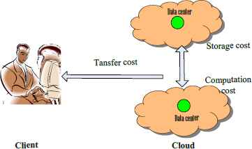
Data access pattern in the cloud.
In a commercial cloud computing paradigm, if clients want to deploy and run applications, they need to pay for the resource used. In practice, especially in science workflow application, the traditional remote call mode is not suitable, for the reason that various applications may be done with the data sets. The best way is to move data sets to clients’ nearest data center. Also, each data center has many requests for data sets transfers at the same time. We use mi representing the number of clients (tasks) requesting dm via data center dci during a certain time period τ.
In practical application, the total management cost of data set dm includes storage, computation and bandwidth consumption. Based on these factors, we propose a comprehensive cost model that covers all aspects of data set management.
Definition 6.
Total data set management cost of data set dm . The total data set management cost of data set dm during a time period τ, is the sum of its storage cost, transfer cost, and generation cost if needed, written as:
- (i)
TCostdm is the total management cost of data set dm in period τ;
- (ii)
tc_strgdm, the sum of storage cost, is the total cost used to store the data sets on data centers;
- (iii)
tc_trsfdm, the sum of transfer cost, is the total cost for transfer data dm to another data center;
- (iv)
p ∈ {0,1}, p=0 means the status of data set dm is “stored”, while p=1 means the status is “deleted”;
- (v)
tc_gendm, the sum of computation cost, is the total cost for regeneration data set dm from its provSetm.
Next, we will present these costs computational approaches separately in detail.
4.2. Data set storage cost model
The total storage cost tc_strg refers to the disk resource consumption to store data sets, depending on parameters such as CSP’s pricing policy, the size of the data (original data set) and storage time. And the storage cost ration is not a fixed value, but a piecewise function.
Definition 7.
Storage cost function (scf). Storage cost function (scf) on data center dcm can be described as a 4-tuple (itvk, sizelk, sizehk, pk), where,
- (i)
itvk is interval identifier, and k is a integer value from integer 1 to n;
- (ii)
sizelk is the lower storage bound of interval k;
- (iii)
sizehk is the upper storage bound of interval k;
- (iv)
pk is storage price per unit time in interval k .
- (v)
The total storage cost is the storage cost function scf multiplied by data set sizes and their respective storage time during the intervals. Consequently, the data storage cost on data center dcm can be defined as follows.
Definition 8.
Total storage cost (tc_strg). The storage cost of data set dm during a certain time period τ can be defined as follows:
- (i)
l is the minimum integer that guarantees the following condition:
- (ii)
itvk, sizehk and sizelk have the same meaning as in Definition 7;
- (iii)
scf(k) is the CSP’s storage cost function as defined in Definition 7;
- (iv)
τ is the storage time.
In this model, the price varies with respect to data size and storage time on data center. For example, using Amazon S3 for storage pricing (referred to Table 2) and considering that dm has been stored for 6 months with 2TB (2048 GB) data size, then the storage cost is:
Compared to the other storage cost models, interval storage cost ratio is the change in the total cost that arises when the quantity produced changes by one unit. So, it can effectively reflect the real storage cost of a data set.
4.3. Data set transfer cost model
Bandwidth is another type of resource in the cloud. Studies have shown that requests usually follow a fixed shortest path routing to data sources and most routes are stable in days or weeks [25]. And data transfer cost depends on several parameters, such as the data set size, the data set type and the price model applied by CSPs. We first present the data transfer cost function.
Definition 9.
Data transfer cost function (tcf). Data transfer cost function (tcf) can be defined as a 5-tuple (itvk, type, sizelk, sizehk, pk), where,
- (i)
itvk is interval identifier, and k is a integer value from integer 1 to n;
- (ii)
type∈{input, output}, means the type of transferred data sets;
- (iii)
sizelk, sizehk, means the lower and upper transfer size bound of interval k separately;
- (iv)
pk is the data transfer cost ration in interval k.
In this way, the total transfer cost tc_ trsfdm is the product of the CSP’s atomic transfer cost function by the total size of transferred data.
Definition 10.
Data transfer cost (tc_trsfdm). Data set transfer cost of data set dm can be defined as:
- (i)
itvk, sizehk and sizelk have the same meaning as in Definition 9;
- (ii)
tcf(k) is the CSP’s transfer cost function as defined in Definition 9, where k is the interval index;
- (iii)
l is the minimum integer that guarantee the following condition:
Moreover, recall the Amazon EC3’s transfer cost is variable. It is free for the first GB. Then, it becomes $0.12 up to 10TB, and so on (Section 2.2). For example, using Amazon EC3’s data sets transfer cost model and considering that dm with 10TB data size is transferred from current data centers to another, and then the cost is: tc_trsfdm=0×1+0.12×(10-1)=$1.08.
4.4. Data set computation cost
Computation cost, also called generation computation cost, is taken by the computation resources consumption on data center. Each data center may bear different performance (with respect to CPUs’ number of CPUs, its available RAM, etc.), and thus different computation cost policy. In this way, to calculate this cost, we have to multiply the time of generating data set dm by the price of computation resources.
Definition 11.
Computation cost function (ccf). Computation cost function (ccf) can be defined as a 3-tuple (k, type, pk), where,
- (i)
k means index identifier;
- (ii)
type is data center configurations types;
- (iii)
pk is the computation cost in configuration type.
Based on the computation cost function, we can define the data set generation cost from its direct predecessor.
Definition 12.
Data set computation cost from its direct predecessor (dp_gen). Generation cost for a data set dm is proportional to its CPU instance time t and CPU computation cost function ccf(dci), and can be described as:
- (i)
dp_gendm denotes the generation cost of data set dm from its direct predecessors;
- (ii)
ccf(dci) is computation cost function, where dci is ithdata center;
- (iii)
t is the amount of time spent for generating data set dm, can be obtained from the system logs.
In this paper, we only consider the linear generation relation for the sake of simplification. And further, not all the data sets are stored in the cloud, in other words, some data sets’ status are “deleted” according to their usage frequency and other cost constraints. In this case, when we want to regenerate a data set in DDG, we have to start the computation from the data set in its provSet. Hence, for data set dm, its generation cost can be defined as follows.
Definition 13.
Generation cost for data set dm (tc_gen). A data set di’s generation cost from its provSet can be described as:
- (i)
tc_gendm is the total generation cost each time;
- (ii)
dp_gendm is the generation cost from its direct predecessor;
- (iii)
dk is a data set from dm’s provSetm whose states are “deleted”.
From above, we can easily know that tc_gendm is a total cost of (1) the generation cost of data set dm from its direct predecessor data set, and, (2) the generation costs of dm’s deleted predecessors that need to be regenerated as well.
5. Trade-off between data set replicas and pseudo-replicas placements from cost view
Different replicas placements strategies lead to different management costs in the cloud. In this section, we will present a trade-off between real-replicas and pseudo-replicas from cost-effective view, if a decision to add a replica has been made.
It must be noted that optimal replicas placements solutions may not be unique. Our goal is to decide real-or pseudo-replicas for data set dm, such that overall data management cost, is minimized for a given client access pattern. Such an ideal solution is shown in Fig 5.

An Example of data access domain.
In Fig 5, we define a data set dm’s placement dci and its neighbor data centers accessing dm from dci as a domain SDi. For example, domain SD1 and SD2 supplies a real data set replica in data center dco and dcp separately, while SD3 is an access domain with a pseudo-replica and its provenance is stored in dcq.
5.1. Data set management cost with real replicas
For simplicity, we will ignore the dynamic changes of factors, such as usage frequencies from different data centers, and regard as static values during a certain time period τ. Also, we assume that the dm’s access times via data center dci follow Poisson distributions with parameter λi within a certain time period τ. It is known that the Poisson distribution can be represented as:
Then, the probability of accessing k times is P(x=k), abbreviated as P(k). And the expectations of total access times Ni from data center dci during τ can be obtained by following expression:
From this way, the total transfer cost of data set dm can be easily obtained theoretically by calculation using the following expressions:
It is obvious that the storage cost will be increased with the existence of data set dm’s replica dm′, for the reason that replica dm′ also cause extra storage resource consumption on destination data center. Therefore, the total storage cost is the sum cost for storage data set dm and its replicas, and can be represented as follows:
5.2. Data set cost model with pseudo-replicas
Next, consider the situation that there is no real data set replicas but a pseudo-replica, in other words, the data set dm will be generated instantly once a request comes for data set dm. As a consequence, the total cost of data set dm includes the generation cost and the transfer cost (the provenance’s storage cost has nothing to data set dm’ management cost). This tactic can efficiently save storage resource and benefit from the computing performance of the cloud. Without the replicas created in the cloud, the storage cost is only caused by data set dm (as an original data set, dm always be stored).
In general, the generation cost is directly proportional to the regeneration times required for client’s requests during a certain time period τ. Then, to calculate the regeneration cost of data set dm (as defined in Definition 13), we have to multiply the times of generation dm by the price of computation cost each time. In addition, total transfers cost is the cost from the data center occupied its provenance provSetm to the client’s side.
In this way, the total data management cost for data set dm can be represented using the following formula:
5.3. Algorithm for tradeoff between data set replica and pseudo-replica
In practice, it is not an easy decision for data set dm’s real- or pseudo-replicas strategy, for the reason of complex data dependency relations and dynamic usage frequencies. However, to find the tradeoff between a real and pseudo-replica, no matter how complex the data sets relationships are, we can deduce the problem to a simple one: measuring the cost by calculation and comparing them.
As a preliminary approach, we first measure the tradeoff between data set replicas or regeneration necessity with only one replica. The main idea is to compare the data set replica cost and generation cost, then to choose the one with less expense. Algorithm 1 presents the way how to decide real or pseudo-replica from cost-effective view.
In the end of Algorithm 1, a result of real or pseudo replica will be presented by comparing the different management cost, along with the real replica or its provenance stored place. In Line 23, function min(tc_trsfdci, dp_gendm +tc_trsf′dci) returns the small value from real replica and its generation approach.
And then, we will analyze the time complexity of Algorithm 1. A simple implementation using an adjacency matrix graph representation and searching an array of weights to find the minimum weight edge to add requires O(|V|2) running time. And tentatively placing data set replica on different data centers such as Line 12 takes n2 steps. So, the total time complexity of Algorithm 1 is O(n2).
| Input: | Data set dm, its stored data center dci and its provenance provSetsm; |
| Testing period τ; | |
| Data access frequency parameter λi via data center dci; | |
| Data centers’ storage, transfer and computation pricing policy. | |
| Output: | The replica strategy: real or pseudo-replica; if real replica then output the replica storage location r_Loc, else output the provenance location. |
| 01. | Calculate the storage cost tc_strgdm based on Definition 8; |
| 02. | Calculate the transfer cost trsfdm based on Definition 10; |
| 03. | For each data center dcj (except data center dc0) |
| 04. | Set tc_trsfdm= tc_trsfdm+λj×trsfdm; |
| 05. | EndFor |
| 06. | Set TCost= tc_strgdm + tc_trsfdm; |
| 07. | For each data center dcj (except data center dc0) |
| 08. | Begin |
| 09. | Create a temporary replica dm′ and store it on data center dcj; |
| 10. | Calculate the storage cost tc_strgdm′ based on Definition 8; |
| 11. | For each data center dck(except data center dc0 and dcj) |
| 12. | Set tc_trsfdm′=tc_trsfdm′+λk×min(tc_trsfdci, tc_trsf′dci); |
| 13. | EndFor |
| 14. | Set TCost′= tc_strgdm+tc_strgdm′+ tc_trsfdm′; |
| 15. | If TCost> TCost′ Then |
| 16. | Set TCost=TCost′ |
| 17. | Set r_Loc=j; |
| 18. | EndIf |
| 19. | EndFor |
| 20. | Calculate the computation cost dp_gendm based on Definition 12; |
| 21. | For each data center dcj (except data center i) |
| 22. | Begin |
| 23. | Tc_trfs_gen= Tc_trfs_gen+λk×min(tc_trsfdci, dp_gendm +tc_trsf′dci); |
| 24. | EndFor |
| 25. | Set TCost″= Tc_trfs_gen +tc_strgdm; |
| 26. | If TCost> TCost″ Then |
| 27. | Print “Create a replica on data center ”+r_Loc |
| 28. | Else |
| 29. | Print “Pseudo-replica strategy, and data provenance ” |
| 30. | EndIf |
| 31. | End |
One real or pseudo replica measurement from cost-effective view
6. GA-based combination replicas placements strategy in cloud environment
In the previous sections, we will present the preliminary cost benchmarking approaches in the cloud, which is the theoretical minimum cost with only one replica. However, it is not an easy question to determine the number and storage places for real-replicas and pseudo-replicas configurations to make sure the total management cost is minimal during a certain time period τ, for the dynamic nature of the cloud computing system, i.e. (i) new data sets may be generated in the cloud at any time; and (ii) the usage frequencies of the data sets may also change as time goes on.
In this part, we will propose a general replicas placements strategy generating optimal or near-optimal solutions for replicas based Genetic algorithms, including fitness function, selection-procedure, mutation operator and replacement population method.
6.1. Minimum management cost model for replicas placements strategy
In this paper, we do not consider nodes capacity constraint, message losses, nodes failures, and the consistency maintenance issues. The communication cost introduced by replicas placements and de-allocation is also not considered. In this way, the data sets replicas placements strategy with minimum cost is NP-hard. Hence, calculating the minimum cost benchmark between real- and pseudo-replicas is a seemingly NP-hard problem based on the cost models introduced in Section 4.
Theorem 1.
For a data set dm, its replicas placements problem with the minimum cost is NP-Hard.
Proof.
We can map the data centers to a graph G(V, E): the data set dci are mapped as node vi, and all nodes constitute a set V={dc1,dc2, dc3,…, dcn};
E={e1, e2, e3, …, ep}, ek represents the connection from dci to dcj, and the weigh is transfer cost multiplied by transfer times;
S represents the data centers set with data set replicas, S⊆V;
∀s∈S, Ds={dcs1, dcs2, … } means the data centers access from data center Ds.
Then, the minimum cost replicas placements strategy can be modeled as follows:
- (i)
Ds≠∅, and
- (ii)
λi is the request times on data center dci;
- (iii)
tc_trsfdm is the transfer cost each time;
It is obvious that the objective function of the data management cost with replicas is identical to the location problems. However, the major models, such as Fixed Charge Location Model, the Covering Model in None-Competitive Location Theory and the Medianoid and Centroid Model [28,29] from Competitive Location theory, are all NP-Hard, i.e. computationally difficult, combinatorial optimization problems. In this way, for a data set dm, its replicas placements problem with the minimum cost is NP-Hard.
Theorem 2.
For a data set dm, the minimum cost real- and pseudo-replicas placements strategy is NP-Hard.
Proof.
As a specific circumstance, we define each data set’s generation cost as 0, then the minimum cost for real and pseudo replicas strategy is the same as the minimum cost for replicas placements strategy, as is shown in Theorem 1. Accordingly, we know that the minimum cost for replicas and pseudo-replicas placements strategy is NP-Hard.
Therefore, exact algorithms are computationally feasible only for medium sized problems or for special cases, not include the general cases [30]. As a result, much research has been devoted to devising heuristic solution procedures which run in reasonable computer time and yield solutions of acceptable quality.
6.2. GA-based heuristics for replicas placements strategy in cloud environment
Genetic algorithms (GAs) are a family of randomized-search optimization heuristics, which are based on the biological process of natural selection [31, 32]. However, applications of GAs to data sets replicas placements have been relatively few. Furthermore, to the best of our knowledge, a comprehensive study on the comparative performance of GAs on replicas placements models has not been attempted before. This is particularly significant in view of the fact that GAs have proven to be very effective on non-convex optimization problems for which it is relatively easy to assess the quality of a given feasible solution but difficult to systematically improve solutions by deterministic iterative methods [33–34]. Motivated by these considerations, this paper will present the GA-based heuristics for data sets replicas placements strategy from cost view.
6.2.1 Representation scheme and fitness function
The first step in designing a genetic algorithm for a data sets problem is to devise a suitable representation scheme. The representation scheme developed is an nf-bit string as the chromosome structure, where nf is the number of potential data sets replicas placements. A value of 1 for the ith bit implies that a replica is located in the ith data center. The representation of an individual’s chromosome (solution) is illustrated in Fig 6.
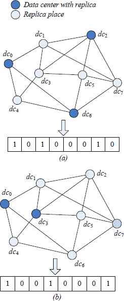
Example of replicas placements chromosome representation.
The data centers network illustrated in Fig 6. has eight data centers. The case (a) represents the situation when three replicas are located in data centers dc0, dc2 and dc6, and case (b) illustrates the situation when replicas are located in data centers dc0 and dc3. In addition, data center dc7 can generate data set from its provenance. The respective binary representations for cases (a) and (b) are also shown in the same figure.
The fitness function in a GA is a measure of goodness of a solution to the objective function. In our modified GA, the fitness of an individual is directly related to its objective function value, which is defined as minimum management cost.
The fitness function value of each possible solution to the replicas placements problem is calculated by finding the set of data centers belonging to the solution being evaluated and adding the demands that are covered by these data centers. Care must be taken in order to avoid demands being counted several times since each data center belongs to only one ds (ds∈DC).
6.2.2 Parents selection-procedure and crossover
We will now address the parents’ selection, i.e., solutions chosen for crossover. And we chose the Binary Tournament Selection Method, for the reasons that: (i) it can be implemented very efficiently; (ii) it has been shown that this method gives solutions whose quality compare favorable to the ones proposed by other methods.
In this paper, we chose the crossover operator fitness-based fusion proposed in [31]. This operator is more capable of generating new solutions when two parent solutions are similar in structure than the one-point crossover operator, since it focuses on the difference in the two structures. However, the possibility of getting an offspring identical to one of its parents still remains. As a result of this problem, the following modification was made to the over all crossover operator. The crossover algorithm can be described as in Algorithm 2.
| Input: | Parents |
| Output: | Crossover result |
| 01. | Select parents p1 and p2; |
| 02. | Apply the fusion operator to obtain an offspring c1; |
| 03. | Compare c1 with its parents. If it is not identical to both of p1 and p2, then go to Step 05. Otherwise, go to Step 4. |
| 04. | Apply mutation to the parent with the lesser fitness. |
| 05. | End |
Crossover
6.2.3 Mutation
Mutation is a process that reverses the structure of a chromosome and hence produces albinos, i.e., individuals with different chromosome properties from the majority in a population. In this work, the mutation operator works by selecting randomly one of the data centers and transferring this to destination data center. The new stored place is also picked randomly from the set of empty possible places to located data storage.
Once new child solutions have been constructed through the GA operators, the child solutions will replace “less fit” members of the population. The average fitness of the population will improve if the child solutions have better fitness than those of the solutions being replaced.
In our GA, we used the incremental replacement method. Using this method, the best solutions are always in the population and the newly created solutions are immediately available for selection and reproduction. Note that when replacing a solution, care must be taken to prevent excessive copies of a solution from entering the population. Allowing too many duplicate solutions to exist in the population may be undesirable because a population could come to consist of identical solutions, thus severely limiting the GAs ability to generate new solutions.
6.3. GA algorithm for minimum data set replicas placements strategy
One of the most obvious questions related to GA performance is how it is influenced by population size. In principle, it is clear that small populations run the disk of seriously uncovering the solution space, while large populations incur severe computational penalties. The experimental work by Alander[35] suggests that a value between n and 2n is optimal for the problem type considered, where n is the length of a chromosome. In this way, we chose a value of n and in our situation the length of a chromosome coincided with the number of possible replicas storage places.
| Input: | Configuration of data set and Data centers |
| Output: | Data set replicas placement strategy |
| 01. | Set t:=0; |
| 02. | Generate initial population, P(t) randomly; |
| 03. | Evaluate each of the strings in P(t) according to the kind of problem being solved. |
| 04. | while (number of generations <=maximum value) or (improvement in objective function value <=10−5) do |
| 05. | Set t:=t+1; |
| 06. | Select two solutions P1 and P2 from the population using binary tournament selection. |
| 07. | apply genetic operators t String P1 and P2, If Crossover: Combine P1 and P2 to form a offspring O1 using the fusion crossover operator. If O1 is identical to any of its parents, then apply mutation operator to the parent with the best fitness. If Mutation: Apply mutation operator to the parent with the best fitness to form an offspring O1. |
| 08. | Repeat steps 6 and 7 until a new set of children is created which is of same size as the parent population. |
| 09. | Evaluate this new child set according to the kind of problem being solved. |
| 10. | Utilize the incremental replacement method to create P(t) from the parent population and set of children. |
GA algorithm for minimum data set replicas placements strategy
Thus, the GA that we implemented can be described algorithmically as follows.
7. Simulations and results analysis
In this section, we describe the overall setup for our preliminary simulations and the results obtained from it. After that, we will present the simulations analysis.
7.1. Simulations setup
The simulations were conduced on a cloud computing simulation environment built on the computing facilitates at Cloud Computing Research Laboratory, Shandong University of Finance and Economics (SDUFE), China, which is constructed based on SwinDeW [36] and SwinDeW-G [37]. The cloud system contains 8 servers (data centers) and 50 high-end PCs (clients), where we install VMWare (http://www.vmware.com), so that it can offer unified computing and storage resources. The heuristics were coded in Java and executed on a PC computer DELL OptiPlex 3020, which is equipped with 1GB of RAM and an Inter ® Core ™ i5-4570M CPU running at 3.2GHz.
We used in our experiments a subset of the data set from our real practice, with each size in the range of [10, 512] GB. And their properties are shown in Table 5. Fig 7 describes the dependency relations of data set d1, d2, d3, d4 and d5. At the very beginning, the number of replicas of each data set is 1 and placed randomly. In order to meet the general requirements, the data sets management price policy is as the same as in the Amazon Simple Storage Service (S3).
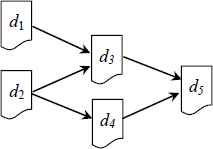
Dependency relation among data sets.
| Data set | Size(G) | Storage place | Storage cost | provSeti |
|---|---|---|---|---|
| d1 | 160 | dc0 | 134.40 | ϕ |
| d2 | 10 | dc2 | 8.40 | ϕ |
| d3 | 80 | dc4 | 67.20 | {d1, d2} |
| d4 | 512 | dc6 | 537.6 | {d2} |
| d5 | 32 | dc7 | 26.88 | {d1, d2}, {d3, d4} |
Properties of data sets
Computation cost of data set is another important element in decide replicas placements strategy, which is depended on the provSet and computational resources price model. Table 6 gives data set dm’s provSetm, their store places and computation costs.
| Data set | provSetm | Computation place | Computation cost per time |
|---|---|---|---|
| d1 | ϕ | / | / |
| d2 | ϕ | / | / |
| d3 | {d1} | dc1 | 89.2 |
| {d2} | dc2 | 120.8 | |
| d4 | {d2} | dc2 | 180.6 |
| d5 | {d3} | dc4 | 32.1 |
| {d4} | dc6 | 24.8 |
Computation cost of data set dm
For calculating the data set transfer cost from its source to the destination, we analyze the data sets transfer process by finding their shortest path. Table 7 gives the data set transfer cost between each pair of data centers.
| Data set | d1 | d2 | d3 | d4 | d5 |
|---|---|---|---|---|---|
| dc0 | 0 | 2.6 | 1.4 | 4 | 5.2 |
| dc1 | 1.4 | 1.4 | 2.4 | 16.6 | 2.4 |
| dc2 | 3.4 | 0 | 3 | 13.2 | 1.6 |
| dc3 | 4 | 1.2 | 1 | 10.6 | 3 |
| dc4 | 1.4 | 4.6 | 0 | 4.4 | 3.6 |
| dc5 | 5.6 | 3 | 3.2 | 5.6 | 2 |
| dc6 | 4.4 | 4 | 1.2 | 0 | 1.4 |
| dc7 | 2.6 | 2.6 | 3 | 5.2 | 0 |
Data set transfer cost each time
Also, the average monthly data transfer requests between these data centers has been illustrated in Table 8.
| Data set | d1 | d2 | d3 | d4 | d5 |
|---|---|---|---|---|---|
| dc0 | 8 | 10 | 12 | 4 | 6 |
| dc1 | 8 | 20 | 16 | 8 | 8 |
| dc2 | 10 | 18 | 18 | 2 | 6 |
| dc3 | 18 | 16 | 14 | 6 | 12 |
| dc4 | 4 | 30 | 10 | 8 | 18 |
| dc5 | 20 | 20 | 6 | 8 | 40 |
| dc6 | 10 | 10 | 6 | 8 | 42 |
| dc7 | 6 | 12 | 4 | 12 | 8 |
Data sets requests frequencies on different data centers
On the other hand, the storage cost on each data center is an important element to be considered. In order to simplify problem, all the data centers take the same storage price model, which varies with respect to its data size. Note that original data sets are stored for the whole considered storage period of six months.
In this way, by using these values, we can apply the total data management cost per month for the case without replicas. Such is illustrated in Table 9.
| Data set | d1 | d2 | d3 | d4 | d5 |
|---|---|---|---|---|---|
| Storage Cost | 134.4 | 8.4 | 67.2 | 537.6 | 26.88 |
| Transfer Cost | 588.8 | 684.8 | 323.2 | 762.4 | 599.2 |
| Total Cost | 723.2 | 693.2 | 390.4 | 1300 | 626.08 |
Data sets transfer cost each time
7.2. Simulations
Based on the configurations above, three kinds of different simulations were applied to replicas placements strategy. First, the data management cost elements and their comparison with different access frequencies. Second, the validity and feasibility of real-replicas and pseudo-replicas strategy were compared against that of sole replicas strategy achieved in the past. Third, in order to see the characteristics of convergence of heuristic proposed and its performance on real-life problems, each heuristic was used to solve a real-world problem. Fig 8 presents the interface of combination data set replicas strategy system.
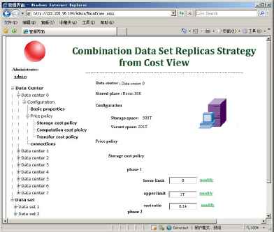
The System interface of combination data set replicas strategy.
7.2.1 Simulation 1: Data management cost factors values comparison
Fig 9 describes the total storage cost, transfer cost and total cost with different number of replicas, from where we can see that the storage cost is less than transfer cost at the beginning, for the reason that much data be transferred in the system. However, with the replicas number increased, the storage cost gradually grows larger for the reason that more replicas need to be stored on data centers. Also, the total cost has a minimum value with three replicas, which means the optimal solution in this circumstance.

Storage cost, transfer cost and total cost with different number of replicas.
Next, we will present the pseudo-replicas strategy under different data sets usage frequencies, as shown in Table 10. In this circumstance, the data set storage cost is only for the original data set, while the computation cost will gradually increase with the number of requests increased.
| Data set requested times | Storage cost | Computation and Transfer Cost |
Total cost | |
|---|---|---|---|---|
| Computation cost | Transfer cost | |||
| 10 | 134.4 | 50.4 | 168.4 | 353.2 |
| 20 | 134.4 | 100.8 | 350.9 | 586.1 |
| 30 | 134.4 | 151.2 | 400.56 | 686.16 |
| 40 | 134.4 | 201.6 | 484.6 | 820.6 |
| 50 | 134.4 | 252 | 548.9 | 935.3 |
| 60 | 134.4 | 302.4 | 688.4 | 1125.2 |
| 70 | 134.4 | 352.8 | 729.5 | 1216.7 |
Data set management cost with pseudo-replicas
Fig 10 illustrates the data management cost comparison with different number of data set requests, from where we can see that (1) the storage cost is a fixed value for the reason that the cost is only for the original data set; (2) the computation cost and transfer cost will grow with the requested number increased for the reason that the computation cost is proportional to the number of generation.
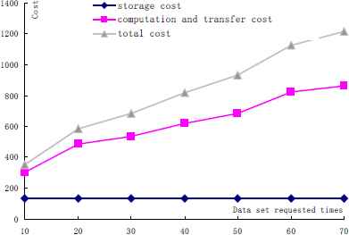
Data management cost with different number of data set requests.
7.2.2 Simulation 2: Feasibility and effectiveness of replicas and pseudo-replicas strategy
In order to evaluate the performance of combination replicas strategy, we have run a large number of simulations with different parameters settings. We present some representative results in this sub-section. Table 11 summarizes the simulations results of real-replicas strategy and pseudo-replica strategy. In this table, we list the best replicas solution and pseudo-replica solution, such as replicas numbers, their storage places, the average CPU solution time, etc al.
| Data sets | Best replicas solution (without pseudo-replica) | Replicas and pseudo-replicas solution | ||||||||
|---|---|---|---|---|---|---|---|---|---|---|
| Replicas number (include original data set) | Storage place | Mean CPU time(s) | Total cost | Replicas | Pseudo-replica | Mean CPU time(s) | Total cost | |||
| Numbers (include original data set) | Storage Places | Provenance | Storage place | |||||||
| d1 | 3 | dc0, dc4, dc7 | 14.8 | 1737.12 | 3 | dc0, dc4,dc7 | / | / | 15.3 | 1737.12 |
| d2 | 2 | dc2, dc5 | 28.6 | 155.28⎕ | 2 | dc2, dc5 | / | / | 28.6 | 155.28 |
| d3 | 3 | dc1, dc4, dc6 | 42.8 | 882.48⎕ | 2 | dc1, dc6 | d1 | dc4 | 52.4 | 740.63 |
| d4 | 2 | dc2, dc6 | 36.1 | 1886.64 | 2 | dc2, dc6 | / | / | 36.4 | 1886.64 |
| d5 | 1 | dc7 | 28.4 | 547.68⎕ | 1 | dc7 | / | / | 29.5 | 547.68 |
Comparison of replicas strategy and pseudo-replica strategy
From Table 11, the following remarks can be made regarding the results illustrated. (i) The real-replicas and pseudo-replicas solution can reach the better or the same result for all the data sets, compared to the solution without pseudo-replica. Though the mean CPU time is bigger than the traditional replicas solution, the number of replicas and the management cost are both optimal. (ii) The combination of real-replicas and pseudo-replicas strategy can decrease the storage space on data centers, for the reason that the less number of real replicas leads to little storage. In this way, the algorithm reached the same objective function value in all of the instances. These results indicate that the real-replicas and pseudo-replicas placements strategy availability and validity.
To further illustrate the cost reduction between combination strategy and other works, we have designed specifically and exclusively for cost comparison. In the performance evaluation, in addition to the proposed algorithms (GA), we also include the no replication (NREP) scheme as the baseline, random (RAND) scheme and minimum-cost replicas placements algorithm (MCRP)[38] for comparison. As the name states, in NREP there is just the original objects in the root as a replica of data set.
In order to compare the data sets management cost in different strategies, we define the normalized cost (NCk) as the ratio of difference among NREP cost and the cost of the feasible solution founded by the algorithm to the cost of the NREP scheme. It is given by the following formula.

Comparisons of the total data management cost with different replicas placements strategies.
Fig 11 clearly shows a cost cut of proposed replicas strategy over the other algorithms. And it is obvious that the total cost of replicas becomes constant for a certain more number of replicas. As a result, our proposed algorithm optimizes the cost of replication.
Fig 12 shows the convergence of the GA algorithm with different replicas placements strategies. From the result illustrated in Fig 12, we can see that the algorithm arrives at a stable convergence after 200 loops, which takes about 500 seconds. However, this observation should be viewed with caution in light of the facts that (i) the number of data centers is only eight, which is less than the real environment in practice; (ii) the dependency is simple, which is only linear dependency relation, and may be complex in real application.

The convergence of the GA algorithm with different replicas placements strategies.
7.2.3 Simulation 3: the robustness of the combination strategy
In order to testify the robustness of GA algorithm, we design a series of problems with different number of data centers and data sets dependency relations, even to solve real-world problems. The real-world problem is a network that also established in Cloud Computing Research Laboratory. This network has 40 data centers and nearly 200 client computers.
Table 12 depicts each problem, such as data centers numbers, the data sets number, the percentage of optimal solution reached, the optimal management cost, and the corresponding result of tradition replicas strategy.
| Problem | Number of data centers | Number of data sets | Data sets dependency relation | Combination strategy | Replicas strategy | ||
|---|---|---|---|---|---|---|---|
| % of times optimal sol. reached | Mean CPU time (s) | % of times optimal sol. reached | Mean CPU time (s) | ||||
| L-1 | 8 | 10 | Linear | 100 | 28.45 | 100 | 16.24 |
| L-2 | 8 | 10 | Linear | 100 | 32.58 | 100 | 24.51 |
| L-3 | 8 | 10 | Linear | 100 | 38.22 | 100 | 32.54 |
| L-4 | 8 | 10 | Linear | 100 | 40.28 | 100 | 38.56 |
| L-5 | 8 | 10 | Linear | 100 | 48.25 | 100 | 43.86 |
| M-1 | 20 | 30 | Medium | 100 | 68.79 | 98 | 68.00 |
| M-2 | 20 | 30 | Medium | 100 | 76.85 | 97 | 72.35 |
| M-3 | 20 | 30 | Medium | 100 | 86.54 | 95 | 83.33 |
| M-4 | 20 | 30 | Medium | 100 | 99.63 | 90 | 94.56 |
| M-5 | 20 | 30 | Medium | 100 | 100.23 | 89 | 98.65 |
| C-1 | 40 | 60 | Complex | 98 | 140.36 | 90 | 102.53 |
| C-2 | 40 | 60 | Complex | 99 | 160.23 | 85 | 150.21 |
| C-3 | 40 | 60 | Complex | 98 | 180.95 | 82 | 143.25 |
| C-4 | 40 | 60 | Complex | 97 | 200.63 | 83 | 162.53 |
| C-5 | 40 | 60 | Complex | 98 | 220.14 | 82 | 188.56 |
Comparisons of combination replicas strategy and replicas strategy
The GA-based heuristics are run on each data set multiple times since GAs are stochastic and therefore yield different searches and potentially different results, for each random number seed used. Ten different seeds were selected to create 10 genetic runs for each problem. These ten runs tested the dependence of the method on the seed selected, both in terms of solution quality and search effort. When the solution quality showed little sensitivity to the choice of the initial seed, we considered the GAs to be “robust”.
8. Conclusions and further works
Data sets replication techniques are used in cloud computing environment to reduce makespan, storage consumption, access latency and network bandwidth. In this paper, we have investigated data sets replicas features and requirements in the cloud platform based on minimum data management cost. Our criteria in choosing real-replicas and pseudo-replicas strategies were (i) ensure that they are costly effective and validity and as general as possible; (ii) get minimum data management cost under the certain premise in users’ response time; (iii) be applicable and compliant with practicality, for the popular cost model.
Our main contribution is the presentation of a combination strategy based on a comprehensive cost model for hybrid clouds (i.e., some of the enterprise services run on an in-house data centers and some run in the cloud), which is useful for enterprises that own data centers. Theoretical analysis, general random simulations, and specific case studies indicate that our strategy is very cost-effective by achieving close to or even the same as the minimum cost benchmark with highly practical runtime efficiency.
However, this paper presents the first attempt to apply the technique to solve the problem as how to place duplicate copies of data sets on the most appropriate data centers in the cloud from cost-effective view. It must be kept in mind that these findings are the results of a preliminary study. To be more useful in practice, future works can be conducted from the following aspects:
- (i)
The current work in this paper has an assumption that the data sets’ usage frequencies are obtained from the system log. Models of forecasting data set usage frequency can be further studied, with which our benchmarking approaches and replicas strategies can be adapted more widely to different types of applications.
- (ii)
The replicas placements strategy should incorporate the data generation, and de-duplication technology, especially data content based de-duplication technology, which is a strong and growing demand for business to be able to more cost-effectively manage big data while using cloud computing platforms.
Footnotes
This work is partly supported by Shandong Provincial Natural Science Foundation (ZR2016FM01), China; the Doctor Foundation of Shandong University of Finance and Economics under Grant (2010034), and the Project of Jinan High-tech Independent and Innovation (201303015), China.
References
Cite this article
TY  - JOUR
AU  - Xiuguo Wu
PY  - 2017
DA  - 2017/01/01
TI  - Combination Replicas Placements Strategy for Data sets from Cost-effective View in the Cloud*
JO  - International Journal of Computational Intelligence Systems
SP  - 521
EP  - 539
VL  - 10
IS  - 1
SN  - 1875-6883
UR  - https://doi.org/10.2991/ijcis.10.1.521
DO  - 10.2991/ijcis.10.1.521
ID  - Wu2017
ER  -