Fusion of heterogeneous incomplete hesitant preference relations in group decision making

Zhen Zhang; Chonghui Guo

doi:10.1080/18756891.2016.1149999

<Previous Article In Issue

Download article (PDF)

Next Article In Issue>

Volume 9, Issue 2, April 2016, Pages 245 - 262

Fusion of heterogeneous incomplete hesitant preference relations in group decision making

Authors

Zhen Zhang^*^,zhangzhen@mail.dlut.edu.cn, Chonghui Guoguochonghui@tsinghua.org.cn

Institute of Systems Engineering, Dalian University of Technology, Dalian, 116024, China

^*Corresponding author.

Corresponding Author

Zhen Zhangzhangzhen@mail.dlut.edu.cn

Received 28 October 2015, Accepted 8 January 2016, Available Online 1 April 2016.

DOI: 10.1080/18756891.2016.1149999 How to use a DOI?
Keywords: preference relation; hesitant fuzzy set; group decision making; logarithmic least squares
Abstract: In this paper, we focus on the fusion of heterogeneous incomplete hesitant preference relations (including hesitant fuzzy preference relations and hesitant multiplicative preference relations) under group decision making settings. First, some simple formulae are developed to derive a priority weight vector from an incomplete hesitant fuzzy preference relation or an incomplete hesitant multiplicative preference relation based on the logarithmic least squares method. Based on the priority weight vector, an induced fuzzy or multiplicative preference relation can be derived for an incomplete hesitant preference relation. Moreover, the consistency indices of hesitant fuzzy preference relations and hesitant multiplicative preference relations are defined. Afterwards, an approach to group decision making based on incomplete hesitant fuzzy preference relations and incomplete hesitant multiplicative preference relations is developed to deal with group decision making problems with multiple decision organizations. Finally, three examples are used to illustrate the proposed approach.
Copyright: © 2016. the authors. Co-published by Atlantis Press and Taylor & Francis
Open Access: This is an open access article under the CC BY-NC license (http://creativecommons.org/licences/by-nc/4.0/).

1. Introduction

Group decision making (GDM) is a common activity occurring in human beings’ life, which usually needs a group of decision makers to achieve the final decision for a specific decision making problem¹. For actual decision making problems, preference relation is a useful tool for decision makers to express their preferences over alternatives through pairwise comparisons^2,3. In recent years, a number of methods have been proposed to deal with GDM problems with preference relations^4,5,6,7,8.

The fuzzy preference relation is one of the most widely used preference relations for actual decision making problems. Given a set of alternatives X = {x₁, x₂, … , x_n}, the degree to which the alternative x_i is preferred to x_j is characterized by a membership function μ_P(x_i, x_j) ∈ [0, 1], then the fuzzy preference relation over the alternatives is represented by a matrix P = (p_ij)_n×n, where p_ij = μ_P(x_i, x_j). To avoid misleading solutions, two important issues are usually considered for GDM with fuzzy preference relations: (1) Individual consistency which is used to measure the agreement degree among the preference values provided by an individual decision maker⁹; (2) Group consensus which is used to measure the agreement degree among different decision makers’ judgments¹⁰. Up to now, different models for checking and improving the consistency and consensus for fuzzy preference relations have been developed. For instance, Herrera-Viedma et al.¹¹ put forward a new characterization of the additive consistency property of fuzzy preference relations and utilized the property to construct consistent fuzzy preference relations from a set of n − 1 preference values. Ma et al.¹² proposed an analysis method to check and improve the consistency of a fuzzy preference relation based on graph theory. Herrera-Viedma et al.¹³ developed a consensus model for GDM with incomplete fuzzy preference relations by considering both the consensus and consistency measures. Chiclana et al.⁹ defined the cardinal consistency for a fuzzy preference relation and showed that cardinal consistency with the conjunctive representable cross ratio uninorm is equivalent to Tanino’s multiplicative transitivity property¹⁴. Moreover, they concluded that multiplicative transitivity is the most appropriate property for modeling cardinal consistency of a fuzzy preference relation. Wu and Xu¹⁵ developed a concise consensus support model for GDM based on deviation measures of fuzzy preference relations. Xia et al.¹⁶ proposed some consistency and consensus models for GDM with fuzzy preference relations based on multiplicative consistency.

Due to the lack of knowledge and decision makers’ limited expertise, preference relations provided by a decision maker are sometimes incomplete. Thus, how to manage incomplete information for GDM with preference relations is also a quite important issue^{13,17,18,19,20,21}. As surveyed by Ureña et al.²², the technique for dealing with incomplete fuzzy preference relations can be divided into two categories. One is iterative approaches which estimate the missing elements based on the consistency property of fuzzy preference relations^23,24, and the other is to estimate the missing preference values or to directly derive the priority weight vector of alternatives without previously completing the preference relations through establishing some optimization models^{17,18,25,26,27,28}. For a detailed review about these techniques, readers can refer to Ref. 22.

To overcome the limitations of fuzzy sets theory when dealing with imprecise and vague information with different sources of vagueness simultaneously, some extensions of fuzzy sets were proposed by scholars, such as intuitionistic fuzzy sets²⁹, type-2 fuzzy sets³⁰, interval-valued fuzzy sets³¹ and fuzzy multisets³². Considering the common difficulty that often appears when the membership degree of an element must be established and the difficulty is not because of an error margin (as in intuitionistic fuzzy set) or due to some possibility distribution (as in type-2 fuzzy sets)^33,34, Torra and Narukawa^35,36 defined the hesitant fuzzy set, which allows the membership degree of an object to have a set of possible values. The hesitant fuzzy set may be helpful in the following two cases: (1) When providing assessments over alternatives, a decision maker may have some hesitancy due to the uncertainty of the environment and lack of knowledge. In this case, the hesitant fuzzy set can be used to represent the possible assessment values of the decision maker. (2) For a GDM problem conducted within organizations, each member of an organization may be required to provide assessments about the alternatives, then the hesitant fuzzy set can be used to represent the evaluation information of the organization, especially when anonymity is required to protect decision makers’ privacy or avoid influencing each other³⁷.

Since the appearance of hesitant fuzzy sets, much work has been conducted on the aggregation of hesitant fuzzy elements³⁷, distance and similarity measures for hesitant fuzzy sets^38,39 and decision making methods based on hesitant fuzzy sets⁴⁰. In recent years, research on hesitant preference relations has also received more and more attentions³³. For instance, Zhu and Xu⁴¹ proposed the concept of hesitant fuzzy preference relation (HFPR) and developed a regression method to transform HFPRs to fuzzy preference relations with the highest consistency level. Moreover, Liao et al.⁴² investigated the multiplicative consistency of an HFPR and developed some algorithms to improve the group consensus. Based on hesitant fuzzy linguistic term sets⁴³, Zhu and Xu⁴⁴ presented the concept of hesitant fuzzy linguistic preference relation and provided two optimization methods to improve the consistency of a hesitant fuzzy linguistic preference relation. Chen et al.⁴⁵ extended the hesitant fuzzy set to interval-valued hesitant fuzzy set and defined the interval-valued HFPR, based on which they developed an approach to GDM with interval-valued HFPRs. Zhu et al.⁴⁶ proposed some approaches to deriving the ranking of alternatives based on HFPRs using the α-normalization and the β-normalization. Recently, Xia and Xu⁴⁷ defined the concept of hesitant multiplicative elements and hesitant multiplicative preference relation (HMPR) and developed some approaches to managing hesitant information in GDM problems with fuzzy and multiplicative preference relations. For GDM problems with HMPRs, Zhang and Wu⁴⁸ defined the individual consistency index and group consensus index, and then developed a consistency and consensus-based decision support model. Based on the concept of HMPR, Zhu and Xu⁴⁹ proposed the analytic hierarchy process-hesitant GDM approach to deal with decision making problem with hierarchal structures.

The previous research has significantly advanced the research of GDM based on hesitant preference relations. However, there are still some challenges which need to be tackled: (1) For some GDM problems with high uncertainty, decision makers may have limited knowledge about the problems to be solved, and incomplete hesitant preference relations may be provided. However, there is little research focusing on managing incomplete hesitant preference relations. (2) Most traditional approaches derive a ranking of alternatives from a hesitant preference relation based on the aggregation operators of hesitant fuzzy elements and hesitant multiplicative elements, which sometimes are quite complex, as the dimension of the derived hesitant fuzzy/multiplicative elements may increase significantly. (3) Due to the differences of culture and education backgrounds, heterogeneous hesitant preference relations may be provided by different decision makers or organizations. However, there is no study that is devoted to the fusion of heterogeneous (incomplete) hesitant preference relations.^†

The main contribution of this paper is to tackle the three challenges mentioned above, which is summarized as below. First, motivated by the logarithmic least squares method^50,51,52, this paper develops some formulae to derive priority weights from an incomplete HFPR or an incomplete HMPR, and then an approach to GDM based on heterogeneous incomplete hesitant preference relations is proposed, which can be used to deal with GDM problems with multiple decision organizations. The proposed GDM approach avoids the complex operations of hesitant fuzzy elements or hesitant multiplicative elements, and allows decision makers to express their preference information flexibly.

The rest of this paper is organized as follows. In section 2, some preliminaries related to hesitant preference relations are presented. Afterwards, section 3 develops some simple formulae to derive priority weights from an incomplete hesitant preference relation. In section 4, an approach to GDM with incomplete HFPRs and incomplete HMPRs is proposed. Three examples are provided to illustrate the proposed approach in section 5, and section 6 discusses the characteristics of the proposed approach. Finally, some conclusions are drawn in section 7.

2. Preliminaries

In this section, some preliminaries related to HFPRs and HMPRs are presented.

Definition 1. (Saaty 1977)²

Let X = {x₁, x₂, … , x_n} be a fixed set. A multiplicative preference relation over X is represented by a pairwise matrix C = (c_ij)_n×n with c_ij c_ji = 1, 1/9 ⩽ c_ij ⩽ 9, where c_ij denotes the ratio degree to which the alternative x_i is preferred to x_j, i, j ∈ I = {1, 2, … , n}.

Definition 2. (Orlovsky 1978)³

Let X = {x₁, x₂, … , x_n} be a fixed set. A fuzzy preference relation over X is represented by a pairwise matrix D = (d_ij)_n×n with d_ij + d_ji = 1, 0 ⩽ d_ij ⩽ 1, where d_ij denotes the degree to which the alternative x_i is preferred to x_j, i, j ∈ I.

Definition 3. (Tanino 1984)¹⁴

Let D = (d_ij)_n×n be a fuzzy preference relation, then D is called a multiplicatively consistent fuzzy preference relation if d_ij > 0, d_ijd_jkd_ki = d_jid_kjd_ik for all i, j, k ∈ I, and such a fuzzy preference relation can also be given by dij=wiwi+wj, i, j ∈ I, where w = (w₁, w₂,...,w_n)^T is the priority weight vector of D, and w_i > 0, i ∈ I, ∑i=1nwi=1.

Remark 1.

Usually, there are two different scales for a fuzzy preference relation D, including the 0–1 scale (i.e. d_ij ∈ [0, 1], i, j ∈ I) and the 0.1–0.9 scale (i.e. d_ij ∈ [0.1, 0.9], i, j ∈ I). According to Definition 3, d_ij > 0 is usually assumed when the multiplicative consistency of fuzzy preference relations is used. To facilitate the transformation between a fuzzy preference relation and a multiplicative preference relation, the 0.1–0.9 scale is applied in this paper when the multiplicative consistency is used for a fuzzy preference relation.

To allow the membership degree of an object to have a set of possible values, Torra and Narukawa^35,36 defined the hesitant fuzzy set as below.

Definition 4.

Let X be a fixed set, a hesitant fuzzy set on X in terms of a function that when applied to X returns a subset of [0, 1]³⁶. To be easily understood, Xia and Xu³⁷ expressed the hesitant fuzzy set by a mathematical symbol E = {〈x, h_E (x)〉|x ∈ X}, where h_E (x) is a set of some values in [0,1], denoting all the possible membership degrees of the element x ∈ X to the set E. For convenience, h = h_E (x) is called a hesitant fuzzy element.

Definition 5. (Zhu & Xu 2013)⁴¹

Let X = {x₁, x₂, … , x_n} be a fixed set, where x_i denotes the i th alternative, i ∈ I, then an HFPR A over X is denoted by a matrix A = (a_ij)_n×n, where aij={aijs|s=1,2,...,lij} is a hesitant fuzzy element indicating all the possible degrees to which the alternative x_i is preferred to x_j. Moreover, a_ij should satisfy the following conditions:

(1)aijσ(s)+ajiσ(lij−s+1)=1,aijs∈[0,1],aii={0.5},lij=lji,s∈Sij={1,2,...,lij},i,j∈I,

where {σ(1), σ(2),..., σ(l_ij)} is a permutation of {1,2,...,l_ij} such that aijσ(s−1)<aijσ(s), s = 2,3,...,l_ij, i.e. aijσ(s) is the s th smallest element in a_ij, i, j ∈ I.

Based on the multiplicative consistency of fuzzy preference relations (i.e. Definition 3), a multiplicative consistent HFPR is defined as follows.

Definition 6. (Zhu, Xu & Xu 2014) ⁴⁶

Let A = (a_ij)_n×n be an HFPR, where aij={aijs|s=1,2,...,lij} is a hesitant fuzzy element, i, j ∈ I. If the following convex feasible region

(2)Θ={w=(w1,w2,...,wn)T|wiwi+wj∈aij,wi>0,i,j∈I,∑i=1nwi=1}

is non-empty, then A is a multiplicative consistent HFPR.

Remark 2.

According to Remark 1, it is assumed that aijs∈[0.1,0.9] when the multiplicative consistency is used for an HFPR.

Definition 7. (Xia & Xu 2013)⁴⁷

Let X be a fixed set, a hesitant multiplicative set on X is defined as F = {〈x,t_F (x)〉|x ∈ X}, where t_F(x) denotes the set of possible multiplicative preference information of the element x ∈ X to the set F and t_F(x) ⊂ [1/9, 9], ∀x ∈ X. For convenience, t = t_F(x) is called a hesitant multiplicative element.

Definition 8. (Xia & Xu 2013)⁴⁷

Let X = {x₁, x₂, … , x_n} be a fixed set, where x_i denotes the i th alternative, i ∈ I, then an HMPR B over X is denoted by a matrix B = (b_ij)_n×n, where bij={bijs|s=1,2,...,lij} is a hesitant multiplicative element indicating all the possible ratio degrees to which the alternative x_i is preferred to x_j. Moreover, b_ij should satisfy the following conditions:

(3)bijδ(s)bjiδ(lij−s+1)=1,bijs∈[1/9,9],bii={1},lij=lji,s∈Sij={1,2,...,lij},i,j∈I,

where {δ(1), δ(2), … , δ(l_ij)} is a permutation of {1, 2, … , l_ij} such that bijδ(s−1)<bijδ(s), s = 2, 3, … , l_ij , i.e. bijδ(s) is the s th smallest element in b_ij , i, j ∈ I.

As a multiplicative preference relation C = (c_ij)_n×n can be transformed into a fuzzy preference relation D = (d_ij)_n×n by^53,54

(4)dij=cij1+cij,i,j∈I,

the following theorems are introduced to achieve the transformation between an HFPR and an HMPR.

Theorem 1.

Let B = (b_ij)_n×n be an HMPR, then it can be transformed into an HFPR A = (a_ij)_n×n, where aij={aijs|s=1,2,...,lij} and

(5)aijs=bijs1+bijs,s∈Sij,i,j∈I.

Theorem 2.

Let A = (a_ij)_n×n be an HFPR, then it can be transformed into an HMPR B = (b_ij)_n×n, where bij={bijs|s=1,2,...,lij} and

(6)bijs=aijs1−aijs,s∈Sij,i,j∈I.

Theorem 3.

Let A = (a_ij)_n×n be an HFPR. If we first transform it into an HMPR B = (b_ij)_n×n by Eq. (6) and then transform B into an HFPR A′ = (a′_ij)_n×n by Eq. (5), where aij'={aij's,s=1,2,...,lij}, i, j ∈ I, then A = A′.

The proofs of Theorems 1–3 are provided in Appendix A.

Theorem 4.

Let B = (b_ij)_n×n be an HMPR. If we first transform it into an HFPR A = (a_ij)_n×n by Eq. (5) and then transform A into an HMPR B′ = (b′_ij)_n×n by Eq. (6), where bij'={bij's|s=1,2,...,lij}, i, j ∈ I, then B = B′.

Proof.

The proof is similar to that of Theorem 3.

Remark 3.

Theorems 1 and 2 show that an HFPR and an HMPR can be transformed into each other, and Theorems 3 and 4 demonstrate that the transformation is invertible. Note that there are some other approaches to conducting the transformation processes, and the reason why Eqs. (5) and (6) are utilized is that such transformations coincide with the consistency definition of a multiplicative preference relation and a fuzzy preference relation from the priority weight vector perspective, which can result in the priority weight derivation model easily (see the model (15)).

3. Deriving priority weights and consistent preference relations from an incomplete hesitant preference relation

Due to the lack of time and knowledge, decision maker’s limited expertise, or incapacity to quantify the preference degree, incomplete preference relations are usually provided by a decision maker. Motivated by the definition of acceptable incomplete preference relations⁵⁵, we give the definitions of acceptable incomplete HFPRs and acceptable incomplete HMPRs, respectively.

Definition 9.

Let A = (a_ij)_n×n be an HFPR. If some elements of A are unknown, A is called an incomplete HFPR. If there exists at least one known element (except diagonal elements) in each row or each column of A, then A is called an acceptable incomplete HFPR.

Definition 10.

Let B = (b_ij)_n×n be an HMPR. If some elements of B are unknown, we call B an incomplete HMPR. If there exists at least one known element (except diagonal elements) in each row or each column of B, then B is called an acceptable incomplete HMPR.

Up to now, most previous approaches focus on deriving priority weights from a complete HFPR or a complete HMPR, and little work has been conducted on deriving priority weights from incomplete hesitant preference relations. Motivated by the logarithmic least squares method^50,51,52, in this section we develop some formulae to derive priority weights from an incomplete HFPR or an incomplete HMPR. Note that all the incomplete hesitant preference relations considered in this paper are acceptable ones.

First of all, we focus on how to derive priority weights from an incomplete HFPR. Let A = (a_ij)_n×n be an incomplete HFPR. If the element a_ij is known, we denote it as aij={aijs|s=1,2,...,lij}. For the missing elements, let a_ij = φ. For convenience, we introduce the indication matrix Δ = (δ_ij)_n×n for A to indicate whether the elements of A are known or not, where

(7)δij={1for aij≠ϕ0for aij=ϕ,i,j∈I.

Motivated by Ref. 46 and Definition 6, if A is consistent, we have

wiwi+wj∈aij, for all δij=1,i,j∈I,

i.e.

δijwijwi+wj=δijaij1 or δijaij2 or ...or δijaijlij,i,j∈I,

which can be written as

δijwiwj=δijaij1ajilij or δijaij2ajilij−1 or ... or δijaijlijaji1,i,j∈I.

As we assume that w_i > 0, i ∈ I, we have

(8)δij(ln⁡wi−ln⁡wj)=δijln⁡aij1ajilij or δijln⁡aij2ajilij−1 or ...or δijln⁡aijlijaji1,i,j∈I.

However, Eq. (8) may usually not hold, i.e. there are some deviations which are calculated as

εijs=δij(ln⁡wi−ln⁡wj−ln⁡aijsajilij−s+1),s∈Sij,i,j∈I.

It is obvious that the values of all the εijs should be kept as small as possible. Therefore, we establish the following optimization model:

(9)min⁡z1=∑i=1n∑j=1n∑s=1lij(εijs)2 =∑i=1n∑j=1n∑s=1lijδij(ln⁡wi−ln⁡wj−ln⁡aijsajilij−s+1)2s.t.∑i=1nwi=1,wi>0,i∈I.

Theorem 5.

Let

(10)D=(∑j=2nl1jδ1j−l12δ12…−l1(n−1)δ1(n−1)−l21δ21∑j=1j≠2nl2jδ2j…−l2(n−1)δ2(n−1)⋮⋮⋮⋮−l(n−1)1δ(n−1)1−l(n−1)2δ(n−1)2…∑j=1j≠n−1nl(n−1)jδ(n−1)j),

and

(11)Y=(∑j=1n∑s=1l1jδ1jln⁡a1jsaj1l1j−s+1∑j=1n∑s=1l2jδ2jln⁡a2jsaj2l2j−s+1⋮∑j=1n∑s=1l(n−1)jδ(n−1)jln⁡a(n−1)jsaj(n−1)l(n−1)j−s+1).

then the solution to the model (9) is w = (w₁, w₂,..., w_n)^T, where

(12)wi={exp⁡(pi)∑j=1n−1exp⁡(pj)+1,i=1,2,...,n−1,1∑j=1n−1exp⁡(pj)+1,i=n.

with P = (p₁,p₂,...,p_n−1) = D⁻¹Y.

The proof of Theorem 5 is provided in Appendix A.

Based on Eq. (12), we can derive a consistent fuzzy preference relation Ā = (ā_ij)_n×n, where a¯ij=wiwi+wj, i, j ∈ I. Here, we call Ā the induced fuzzy preference relation of the HFPR A. The objective function value of the model (9) reflects the consistency level of the HFPR A, i.e. the smaller the value of z₁, the more consistent the HFPR A. Considering the numbers of the known elements, we define the consistency index of A as

(13)CI(A)=1/(z1∑i=1n∑j=1j≠inlijδij)=∑i=1n∑j=1j≠inlijδij∑i=1n∑j=1n∑s=1lijδij(ln⁡wi−ln⁡wj−ln⁡aijsajilij−s+1)2.

Remark 4.

Some authors have already proposed distinct consistency measures for HFPRs, For instance, Liao et al.⁴² and Zhu et al.⁴⁶ first constructed some consistent HFPRs based on the defined consistency property, and then measured the consistency by calculating the distance between the initial preference relation and the consistent preference relation. When calculating the distances, the numbers of the elements in the two preference relations need to be equal and some normalization operations are usually needed, which may distort the initial preference relations.

Unlike their consistency measures, Eq. (13) utilizes the priority weights derived from the HFPR to measure the consistency, which avoids the normalization operations used in previous consistency measures and makes fully use of the original preference information provided by the decision maker. Moreover, it should be emphasized that Eq. (13) can be used to measure the consistency of an incomplete HFPR, while the consistency indices in Refs. 42 and 46 only work well for complete HFPRs.

In what follows, we consider how to derive a priority weight vector from an HMPR. Let B = (b_ij)_{n× n} be an incomplete HMPR. If the element b_ij is known, we denote it as bij={bijs|s=1,2,...,lij} . For the missing elements, let b_ij = φ. Similarly, we also introduce the indication matrix Δ = (δ_ij)_n×n for B to indicate whether the elements of B are known or not, where

(14)δij={1for bij≠ϕ0for bij=ϕ,i,j∈I.

For an HMPR B = (b_ij)_n×n, we rewrite the objective function of the model (9) based on Theorem 1 as

z2=∑i=1n∑j=1n∑s=1lijδij(ln⁡wi−ln⁡wj−ln⁡bijs/(1+bijs)bjilij−s+1/(1+bjilij−s+1))2=∑i=1n∑j=1n∑s=1lijδij(ln⁡wi−ln⁡wj−ln⁡bijs/(1+bijs)1/bijs1+1/bijs)2=∑i=1n∑j=1n∑s=1lijδij(ln⁡wi−ln⁡wj−ln⁡bijs)2.

Therefore, we can construct an optimization model for an HMPR B = (b_ij)_n×n as

(15)min⁡z2=∑i=1n∑j=1n∑s=1lijδij(ln⁡wi−ln⁡wj−ln⁡bijs)2s.t.∑i=1nwi=1,wi>0,i∈I.

Let Q = (q₁, q₂, … , q_n−1)^T = F⁻¹Y′, where F = D and

(16)Y'=(∑j=1n∑s=1l1jδ1jln⁡b1js∑j=1n∑s=1l2jδ2jln⁡b2js⋯∑j=1n∑s=1l(n−1)jδ(n−1)jln⁡b(n−1)js),

in a similar manner, the solution to the model (15) is derived as

(17)wi={exp⁡(qi)∑j=1n−1exp⁡(qj)+1,i=1,2,...,n−11∑j=1n−1exp⁡(qj)+1,i=n,.

Based on Eq. (17), we can derive a consistent multiplicative preference relation B¯=(b¯ij)n×n, where b¯ij=wiwj, i, j ∈ I. We call B¯ the induced multiplicative preference relation of the HMPR B. Similarly, we define the consistency index for the HMPR B = (b_ij)_n×n as

(18)CI(B)=1/(z2∑i=1n∑j=1j≠inlijδij)=∑i=1n∑j=1j≠inlijδij∑i=1n∑j=1n∑s=1lijδij(ln⁡wi−ln⁡wj−ln⁡bijs)2.

Based on the consistency index, the consistency level of an HMPR can also be measured.

Remark 5.

It is worth noting that an induced fuzzy preference relation can also be derived from an HMPR and an induced multiplicative preference relation can be derived from an HFPR. Whether to derive a fuzzy preference relation or a multiplicative preference relation should be determined according to actual situations.

4. GDM based on heterogeneous incomplete hesitant preference relations

In section 3, we have developed some formulae to derive a priority weight vector and an induced fuzzy or multiplicative preference relation from an incomplete hesitant preference relation. For actual GDM problems, different decision makers may prefer to utilize different types of preference relations due to the difference in culture, experience and educational backgrounds. As a result, how to fuse heterogeneous preference information from different sources becomes an important issue in GDM^56,57,58,59. In this paper, we particularly focus on the fusion of heterogeneous incomplete hesitant preference relations, including incomplete HFPRs and incomplete HMPRs.

4.1. The proposed approach

We consider the following GDM problems. Let X = {x₁, x₂, … , x_n} be the set of alternatives, O = {o₁, o₂, … , o_m} be the set of m organizations and λ = (λ₁,λ₂, … , λ_m)^T be the weight vector of the organizations which needs to be determined, where ∑k=1mλk=1 and λ_k ⩾ 0, k ∈ K ={1,2, … ,m}. Decision makers in each organization provide their preference information using fuzzy preference relations or multiplicative preference relations. Here, we assume that decision makes in the same organization use the same type of preference relations. For convenience, let o_k (k ∈ K₁ = {1,2, … ,m₁}) be the decision organizations whose decision makers use fuzzy preference relations and o_k (k ∈ K₂ = {m₁+1, m₁+2, … ,m}) be the decision organizations whose decision makers use multiplicative preference relations. To protect the privacy of the decision makers, the preference information of each organization is denoted as an HFPR or an HMPR. Let the HFPR of the k th organization be A^k = (a_{i j,k})_n×n, k ∈ K₁, and the HMPR of the k th organization be B^k = (b_{i j,k})_n×n, k ∈ K₂. If the alternatives x_i and x_j are compared by the k th organization (k ∈ K₁), then aij,k={aij,ks|s=1,2,...,lijk} is a hesitant fuzzy element; if the alternatives x_i and x_j are compared by the k th organization (k ∈ K₂), bij,k={bij,ks|s=1,2,...,lijk} is a hesitant multiplicative element. If no comparison between the alternatives x_i and x_j is provided by the k th organization, let a_{i j,k} = φ or b_{i j,k} = φ, k ∈ K.

As the hesitant preference relations are heterogeneous and some elements of the hesitant preference relations are missing, we cannot aggregate them into a collective one directly. To deal with this problem, we propose a novel procedure to fuse heterogeneous incomplete hesitant preference relations. The basic ideas are as follows.

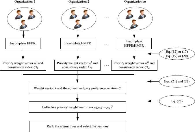
By Eqs. (12) and (17), a priority weight vector which reflects the hesitant preference information of a decision organization can be derived from each HFPR or HMPR. Based on these priority weight vectors, some induced consistent fuzzy preference relations (or multiplicative preference relations) can be obtained^‡, which are homogeneous and complete.

By fusing these induced fuzzy preference relations (or multiplicative preference relations), the collective preference relation is derived. Finally, a collective priority weight vector can be calculated based on the collective preference relation, and then the alternatives can be ranked.

Based on the above analysis, the following GDM approach (Approach I) is developed, as illustrated by Figure 1.

Approach I

Step 1:
Calculate the indication matrices Δk=(δijk)n×n for each organization, where
δijk={1for aij,k≠ϕ0for aij,k=ϕ,i,j∈I,k∈K1,
and
δijk={1for bij,k≠ϕ0for bij,k=ϕ,i,j∈I,k∈K2.
Step 2:
Derive the priority weight vector of each individual hesitant preference relation as wk=(w1k,w2k,...,wnk) by Eq. (12) for all k ∈ K₁ and Eq. (17) for all k ∈ K₂, respectively, and then derive the induced fuzzy preference relation for each organization as Ā^k = (ā_ij,k)_n×n, where a¯ij,k=wikwik+wjk, i, j ∈ I, k ∈ K.
Step 3:
Calculate the consistency index for each HFPR by Eq. (13) as
(19)CIk=CI(Ak)=∑i=1n∑j=1j≠inlijkδijk∑i=1n∑i=1n∑s=1lijkδijk(ln⁡wik−ln⁡wjk−ln⁡aij,ksaji,klijk−s+1)2,k∈K1,
and calculate the consistency index for each HMPR by Eq. (18) as
(20)CIk=CI(Bk)=∑i=1n∑j=1j≠inlijkδijk∑i=1n∑i=1n∑s=1lijkδijk(ln⁡wik−ln⁡wjk−ln⁡bij,ks)2,k∈K2,
Step 4:
Derive the weight vector of the organizations as λ = (λ₁, λ₂, … , λ_m)^T, where
(21)λk=CIk∑h=1mCIh, k∈K.
Step 5:
Aggregate the individual induced fuzzy preference relations of each organization to obtain the collective fuzzy preference relation C = (c_ij)_n×n⁶⁰, where
(22)cij=∏k=1m(a¯ij,k)λk∏k=1m(a¯ij,k)λk+∏k=1m(a¯ji,k)λk,i,j∈I.
Step 6:
Derive the priority weight vector w = (w₁, w₂,..., w_n)^T by⁶¹
(23)wi=∏j=1n(cijcji)1/n∑i=1n(∏j=1n(cijcji)1/n),i∈I.
Step 7:
Rank the alternatives based on w and select the best alternative.

5. Illustrative examples

In this section, we present three examples to illustrate the proposed GDM approach.

Example 1.

First, we consider the supplier selection problems in high-tech companies. Suppose that a high-tech company which manufactures electronic products intends to select a supplier of USB connectors (adapted from Ref. 64). There are four suppliers x₁, x₂, x₃ and x₄ to be selected. Three departments of the company including finance department (o₁), engineering department (o₂) and quality control department (o₃) are invited to evaluate the four suppliers. The experts in each department provide their preference information over the alternatives using fuzzy preference relations or multiplicative preference relations, and experts in the same department use the same type of preference relation. After collecting the preference information of the experts in each department, three heterogeneous incomplete hesitant preference relations are obtained, as listed in Tables 1–3.

o₁	x₁	x₂	x₃	x₄
x₁	{0.5}	{0.3,0.5}	φ	{0.7}
x₂	{0.5,0.7}	{0.5}	{0.25,0.5}	{0.6,0.7}
x₃	φ	{0.5,0.75}	{0.5}	{0.5,0.7}
x₄	{0.3}	{0.3,0.4}	{0.3,0.5}	{0.5}

Table 1:

HFPR (A¹) of the organization o₁

o₂	x₁	x₂	x₃	x₄
x₁	{0.5}	{0.3}	{0.3, 0.6}	{0.5,0.6,0.7}
x₂	{0.7}	{0.5}	{0.3,0.6}	φ
x₃	{0.4, 0.7}	{0.4,0.7}	{0.5}	{0.4,0.6}
x₄	{0.3,0.4,0.5}	φ	{0.4,0.6}	{0.5}

Table 2:

HFPR (A²) of the organization o₂

o₃	x₁	x₂	x₃	x₄
x₁	{1}	{1/2,1}	{1/3, 1/2}	{1}
x₂	{1,2}	{1}	{1,2,3}	{2}
x₃	{2,3}	{1/3,1/2,1}	{1}	φ
x₄	{1}	{1/2}	φ	{1}

Table 3:

HMPR (B³) of the organization o₃

In what follows, we use the proposed approach to deal with the decision making problem. First of all, we derive the indication matrices as follows:

Δ1=(1101111101111111), Δ2=(1111111011111011), Δ3=(1111111111101101).

Afterwards, we calculate the priority weight vector for each hesitant preference relation. Let us take the HFPR A¹ as an example. By Eq. (10), we calculate D and Y for A¹ as

D=(3−20−26−20−24), Y=(01.00141.9459).

Therefore, the priority weight vector of HFPR A¹ is derived as w¹ = (0.2282, 0.2731, 0.3393, 0.1594)^T, and the induced fuzzy preference relation Ā¹ can be calculated as

A¯−1=(0.50.45520.40210.58880.54480.50.44590.63150.59790.55410.50.68040.41120.36850.31960.5).

Similarly, we also derive the priority weight vectors and the induced fuzzy preference relations of A² and B³ as follows:

w2=(0.2327,0.2981,0.2754,0.1938)T,w3=(0.1733,0.3726,0.2744,0.1797)T,

A¯2=(0.50.43840.45790.54560.56160.50.51970.60600.54210.48030.50.58710.45440.39400.41290.5),A¯3=(0.50.31750.38720.49100.68250.50.57590.67460.61280.42410.50.60420.50900.32540.39580.5).

The consistency indices of the hesitant preference relations are calculated by Eqs. (19) and (20) as CI(A¹) = 4.0301,CI(A²) = 3.1107,CI(B³) = 4.6665. Therefore, the weight vector of the organizations is derived as λ = (0.3413, 0.2635, 0.3952)^T.

Based on the induced fuzzy preference relations and the weight vector of the organizations, the collective fuzzy preference relation is calculated as

C=(0.50.39440.41060.53900.60560.50.51690.64230.58940.48310.50.62660.46100.35770.37340.5).

By Eq. (23), the priority weight vector of the four alternatives is obtained as w = (0.2072, 0.3182, 0.2974, 0.1772)^T. Therefore, the best supplier is x₂.

To further illustrate the effectiveness of the proposed approach, we make some comparisons with the approaches developed by Xia & Xu⁴⁷.

Example 2. ⁴⁷

Consider a problem of selecting a loading-hauling system for a hypothetical iron ore open pit mine. Three potential transportation system alternatives are evaluated, i.e. x₁: shoveltruck system, x₂: shovel-truck-in-pit crusher-belt conveyor system and x₃: loader truck system.

Three decision organizations provides their HF-PRs for the three alternatives, as shown in Tables 4–6.

o₁	x₁	x₂	x₃
x₁	{0.5}	{0.1,0.3,0.4}	{0.4,0.6,0.7,0.8}
x₂	{0.6,0.7,0.9}	{0.5}	{0.5,0.6,0.9}
x₃	{0.2,0.3,0.4,0.6}	{0.1,0.4,0.5}	{0.5}

Table 4:

HFPR (A¹) of the organization o₁

o₂	x₁	x₂	x₃
x₁	{0.5}	{0.2,0.4}	{0.5,0.6,0.8}
x₂	{0.6,0.8}	{0.5}	{0.5,0.6,0.8,0.9}
x₃	{0.2,0.4,0.5}	{0.1,0.2,0.4,0.5}	{0.5}

Table 5:

HFPR (A²) of the organization o₂

o₃	x₁	x₂	x₃
x₁	{0.5}	{0.3,0.4,0.5,0.7}	{0.5,0.8}
x₂	{0.3,0.5,0.6,0.7}	{0.5}	{0.5,0.8,0.9}
x₃	{0.2,0.5}	{0.1,0.2,0.5}	{0.5}

Table 6:

HFPR (A³) of the organization o₃

Next, we utilize the proposed approach to deal with this GDM problem. By Eq. (12), the induced fuzzy preference relations of the three HFPRs are derived as

A¯1=(0.50.3006058150.69940.50.76370.41850.23630.5),A¯2=(0.50.33920.60940.66080.50.75240.39060.24760.5),A¯3=(0.50.45170.70650.54830.50.74490.29360.25510.5).

By Eq. (21), the weight vector of the three organization is derived as λ = (0.2803,0.3773,0.3423)^T. Thus, the collective fuzzy preference relation is calculated as

C=(0.50.36480.63660.63520.50.75310.36340.24690.5).

By Eq. (23), the priority weights of the three alternatives can be derived as w₁ = 0.3019, w₂ = 0.5257, w₃ = 0.1724. Therefore, the ranking of the alternatives is x₂ ⥼ x₁ ⥼ x₃, which demonstrates that x₂ is the best alternative. The ranking is also consistent with that derived by Xia & Xu’s approach⁴⁷. However, by contrast, we find that the approach in Ref. 47 is based on the operations of hesitant fuzzy elements, which is more complex than the proposed approach, as the dimension of the derived hesitant fuzzy elements by the operations in Ref. 47 may increase significantly. Moreover, the approach in Ref. 47 can only deal with GDM problems based on complete HFPRs.

Example 3.

Reconsider Example 2. If the preference information of the three decision organizations are provided in the form of HMPR, as demonstrated in Tables 7–9⁴⁷, the following results are obtained.

o₁	x₁	x₂	x₃
x₁	{1}	{1/8,1/5,1/2}	{3,5,7,9}
x₂	{2,5,8}	{1}	{4,6,9}
x₃	{1/9,1/7,1/5,1/3}	{1/9,1/6,1/4}	{1}

Table 7:

HMPR (B¹) of the organization o₁

o₂	x₁	x₂	x₃
x₁	{1}	{1/5,1/2}	{5,6,8}
x₂	{2,5}	{1}	{2,4,7,9}
x₃	{1/8,1/6,1/5}	{1/9,1/7,1/4,1/2}	{1}

Table 8:

HMPR (B²) of the organization o₂

o₃	x₁	x₂	x₃
x₁	{1}	{1/7,1/5,1/4,1/3}	{2,4}
x₂	{3,4,5,7}	{1}	{3,8,9}
x₃	{1/4,1/2}	{1/9,1/8,1/3}	{1}

Table 9:

HMPR (B³) of the organization o₃

By Eq. (17), the induced fuzzy preference relations of the three HMPRs are derived as

A¯1=(0.50.27720.79180.72280.50.90840.20820.09160.5),A¯2=(0.50.37880.80050.62120.50.86810.19950.13190.5),A¯3=(0.50.20830.66590.79170.50.88340.33410.11660.5).

The weight vector of the three organization is derived as λ = (0.2541, 0.2499, 0.496)^T. Therefore, the collective fuzzy preference relation can be calculated as

C=(0.50.26320.73670.73680.50.88680.26330.11320.5).

By Eq. (23), the priority weights of the three alternatives are derived as w₁ = 0.2406, w₂ = 0.6734, w₃ = 0.086, which results in a ranking x₂ ⥼ x₁ ⥼ x₃. Therefore, x₂ is the best alternative, which is also consistent with that shown in Ref. 47.

6. Discussions on the proposed approach

In this section, we make some discussions to show the characteristics of the proposed approach. Compared with previous approaches, the proposed approach has the following advantages.

(1)
The proposed approach is a first attempt to fuse heterogeneous incomplete hesitant preference relations. By literature, we can see that previous work only concentrates on the fusion of complete HFPRs or HMPRs (see Refs. 46,47,48,49). In case of incompleteness and heterogeneity, their approaches will not work well. However, the proposed approach can deal with such cases effectively, which allows decision makers or decision organizations to express their preference information more flexibly. Moreover, when the hesitant preference relations are complete and homogeneous, i.e. only HFPRs or HMPRs, the proposed approach can also be used to derive priority weights (see Examples 2 and 3). Therefore, the proposed approach has more extensive applications in GDM based on hesitant preference relations.
(2)
The proposed approach first uses the logarithmic least squares method to derive an individual priority weight vector and an induced fuzzy (or multiplicative) preference relation from each incomplete hesitant preference relation, and then a collective preference relation is derived by fusing the induced preference relations to output the collective priority weight vector. While the aggregation-based approaches (see Refs. 46,47) utilize hesitant fuzzy aggregation operators or hesitant multiplicative aggregation operators to aggregate the hesitant preference information, which is more complex than the proposed approach, since the dimension of the collective values may increase significantly. Here, we again emphasize that the aggregation-based approaches cannot be used to deal with GDM problems with incomplete hesitant preference relations.
(3)
The priority weights derived by the proposed approach lie in the unit interval. Therefore, the proposed approach can be integrated with the Analytic Hierarchy Process⁶² to deal with multi-criteria decision making problems under GDM settings, especially when the preference information of the decision makers are hesitant, incomplete and heterogeneous.
(4)
The proposed approach also develops a simple formula to determine the weights of decision makers based on the proposed consistency indices, which is helpful when the weight vector of decision makers is unknown.

However, the proposed approach also has some limitations. First, the proposed approach only considers the situations that incomplete hesitant preference relations are acceptable ones, which cannot deal with the ignorance situations that sometimes may appear in actual GDM problems⁶³. Second, the proposed approach can only fuse two types of incomplete hesitant preference relations, which cannot fuse hesitant fuzzy linguistic preference relations⁴⁴. All the issues will be studied in the future.

7. Conclusions

In this paper, based on the logarithmic least squares method, some simple formulae are developed to derive priority weights from an incomplete HFPR or an incomplete HMPR. Based on the individual priority weight vectors, the consistency indices of an HFPR and an HMPR are also defined. To deal with GDM problems with heterogeneous incomplete hesitant preference relations, a novel approach is developed. In the proposed approach, the individual priority weight vector derived from each incomplete hesitant preference relation is utilized to obtain the corresponding induced fuzzy preference relation, and the consistency indices of the incomplete hesitant preference relations are used to determine the weights of decision makers. The proposed approach can allow decision makers or decision organizations to express their preference information more flexibly.

In terms of future research, we intend to integrate hesitant fuzzy linguistic preference relations^44,65 into the GDM approach. Moreover, we will apply the proposed approach to deal with other practical decision making problems, such as company performance appraisal and quality function deployment.

Acknowledgements

The authors would like to thank the Editor-in-Chief, Prof. Luis Mart′ınez and the two anonymous referees for their insightful and constructive comments and suggestions that have led to an improved version of this paper. This work was partly supported by the National Natural Science Foundation of China (Nos. 71501023, 71171030, 61463039), the China Postdoctoral Science Foundation (2015M570248), the Funds for Creative Research Groups of China (No. 71421001) and the Fundamental Research Funds for the Central Universities (DUT15RC(3)003).

Appendix A Proofs of the theorems

Proof of Theorem 1

Proof. Let bijδ(s) be the s th smallest element of b_ij and aijσ(s) be the s th smallest element of a_ij. As f(x)=x1+x is a monotone increasing function of x for all x > 0, we know that bijδ(s)1+bijδ(s) is also the s th smallest element of a_ij, i.e. aijσ(s)=bijδ(s)1+bijδ(s). Moreover, we have

aijσ(s)+ajiσ(lij−s+1)=bijδ(s)1+bijδ(s)+bjiδ(lij−s+1)1+bjiδ(lij−s+1)=bijδ(s)1+bijδ(s)+1/bijδ(s)1+1/bijδ(s)=1,

and aijs∈[0.1,0.9], a_ii = {0.5}, s ∈ S_ij i, j ∈ I. Therefore, A = (a_ij)_n×n is an HFPR.

Proof of Theorem 2

Proof. Let aijσ(s) be the s th smallest element of a_ij and bijδ(s) be the s th smallest element of b_ij . As f(x)=x1−x is a monotone increasing function of x for all x > 0, we know that aijσ(s)1−aijσ(s) is also the s th smallest element of b_ij, i.e. bijδ(s)=aijσ(s)1−aijσ(s). Moreover, we have

bijδ(s)×bjiδ(lij−s+1)=aijσ(s)1−aijσ(s)×ajiσ(lij−s+1)1−ajiσ(lij−s+1)=aijσ(s)1−aijσ(s)×1−aijσ(s)aijσ(s)=1.

As aijs∈[0.1,0.9], we have bijs∈[1/9,9] b_ii = {1}, s ∈ S_ij i, j ∈ I. Therefore, B = (b_ij)_n×n is an HFPR.

Proof of Theorem 3

Proof. By Eq. (6), an HMPR B = (b_ij)_n×n is derived, where bij={bijs|s=1,2,...,lij}={aijs1−aijs|s=1,2,...,lij}, i,j ∈ I. By Eq. (5), we have

aij's=bijs1+bijs=aijs/(1−aijs)1+aijs/(1−aijs)=aijs/(1−aijs)(1−aijs+aijs)/(1−aijs)=aijs,s∈Sij,i,j∈I.

Therefore, A = A′.

Proof of Theorem 5

Proof. To solve the model (9), we construct the following Lagrange function as

L(w,θ)=∑i=1n∑j=1n∑s=1lijδij(ln⁡wi−ln⁡wj−ln⁡aijsajilij−s+1)2+4θ(∑i=1nwi−1),

where θ is the Lagrange multiplier.

Let ∂L∂wi=0, then we have

∑j=1n∑s=1lij4δij(ln⁡wi−ln⁡wj−ln⁡aijsajilij−s+1)⋅1wi+4θ=0,i∈I,

i.e.

(A.1)∑j=1n∑s=1lijδij(ln⁡wi−ln⁡wj−ln⁡aijsajilij−s+1)+θwi=0,i∈I.

Summing both sides of Eq. (A.1) for all i ∈ I, we have

∑i=1n∑j=1n∑s=1lijδij(ln⁡wi−ln⁡wj−ln⁡aijsajilij−s+1)+θ=0,

which is equivalent to

∑i=1n∑j=1n∑s=1lijδij(ln⁡wi−ln⁡wj)−∑i=1n∑j=1n∑s=1lijln⁡(aijsajilij−s+1)δij+θ=0,

i.e.

(A.2)∑i=1n∑j=1nlijδij(ln⁡wi−ln⁡wj)−ln⁡(∏i=1n∏j=1n∏s=1lij(aijsajilij−s+1)δij)+θ=0,

As ∑i=1n∑j=1nlijδij(ln⁡wi−ln⁡wj)=ln⁡∏i=1n∏j=1n(wiwj)lijδij=ln⁡1=0 and ln⁡(∏i=1n∏j=1n∏s=1lij(aijsajilij−s+1)δij)=ln⁡1=0, by Eq. (A.2), we have θ = 0.

Therefore, Eq. (A.1) can be written as

(A.3)∑j=1nlijδij(ln⁡wi−ln⁡wj)=∑j=1n∑s=1lijδijln⁡aijsajilij−s+1,i∈I.

Let

(A.4)D¯=(∑j=2nl1jδ1j−l12δ12⋯−l1nδ1n−l21δ21∑j=1j≠2nl2jδ2j⋯−l2nδ2n⋮⋮⋯⋮−ln1δn1−ln2δn2⋯∑j=1j≠nnlnjδnj)

and

(A.5)Y¯=(∑j=1n∑s=1l1jδ1jln⁡a1jsaj1l1j−s+1∑j=1n∑s=1l2jδ2jln⁡a2jsaj2l2j−s+1⋮∑j=1n∑s=1lnjδnjln⁡anjsajnlnj−s+1),

then Eq. (A.3) is equivalent to

(A.6)D¯P¯=Y¯,

where P¯=(ln⁡w1,ln⁡w2,...,ln⁡wn)T.

As the sum of each row or column of D¯ is zero, D¯ is a singular matrix. Let ln w_n = 0, then we can solve the first n−1 equations of Eq. (A.6). The solution is P = (p₁, p₂, … , p_n−1)^T = (ln w₁, ln w₂, … , ln w_n−1)^T = D⁻¹Y.

Considering the normalization constraint, the solution to the model (9) is derived as Eq. (12). This completes the proof of Theorem 5.

Footnotes

In this paper, when referring to an incomplete hesitant preference relation, it means an incomplete HFPR or an incomplete HMPR, while heterogeneous incomplete hesitant preference relations mean different types of incomplete hesitant preference relations, i.e. HF-PRs and HMPRs.

In the proposed approach, induced fuzzy preference relations are derived.

References

1.RM Rodríguez, L Martínez, and F Herrera, A group decision making model dealing with comparative linguistic expressions based on hesitant fuzzy linguistic term sets, Inf. Sci, Vol. 241, 2013, pp. 28-42.

2.TL Saaty, A scaling method for priorities in hierarchical structures, J. Math. Psychol, Vol. 15, 1977, pp. 234-281.

3.SA Orlovsky, Decision-making with a fuzzy preference relation, Fuzzy Set Syst, Vol. 1, 1978, pp. 155-167.

4.F Herrera, E Herrera-Viedma, and JL Verdegay, A model of consensus in group decision making under linguistic assessments, Fuzzy Set Syst, Vol. 78, 1996, pp. 73-87.

5.F Chiclana, E Herrera-Viedma, F Herrera, and S Alonso, Some induced ordered weighted averaging operators and their use for solving group decisionmaking problems based on fuzzy preference relations, Eur. J. Oper. Res, Vol. 182, 2007, pp. 383-399.

6.Y Dong, Y Xu, and S Yu, Linguistic multiperson decision making based on the use of multiple preference relations, Fuzzy Set Syst, Vol. 160, 2009, pp. 603-623.

7.Y Dong, G Zhang, W Hong, and Y Xu, Consensus models for AHP group decision making under row geometric mean prioritization method, Decis. Support Syst, Vol. 49, 2010, pp. 281-289.

8.Z Zhang and C Guo, Consistency and consensus models for group decision-making with uncertain 2-tuple linguistic preference relations, Int. J. Syst. Sci, 2016.

9.F Chiclana, E Herrera-Viedma, S Alonso, and F Herrera, Cardinal consistency of reciprocal preference relations: a characterization of multiplicative transitivity, IEEE Trans. Fuzzy Syst, Vol. 17, 2009, pp. 14-23.

10.E Herrera-Viedma, FJ Cabrerizo, J Kacprzyk, and W Pedrycz, A review of soft consensus models in a fuzzy environment, Inf. Fusion, Vol. 17, 2014, pp. 4-13.

11.E Herrera-Viedma, F Herrera, F Chiclana, and M Luque, Some issues on consistency of fuzzy preference relations, Eur. J. Oper. Res, Vol. 154, 2004, pp. 98-109.

12.J Ma, Z Fan, Y Jiang, J Mao, L Mao, and L Ma, A method for repairing the inconsistency of fuzzy preference relations, Fuzzy Set Syst, Vol. 157, 2006, pp. 20-33.

13.E Herrera-Viedma, S Alonso, F Chiclana, and F Herrera, A consensus model for group decision making with incomplete fuzzy preference relations, IEEE Trans. Fuzzy Syst, Vol. 15, 2007, pp. 863-877.

14.T Tanino, Fuzzy preference orderings in group decision making, Fuzzy Set Syst, Vol. 12, 1984, pp. 117-131.

15.Z Wu and J Xu, A concise consensus support model for group decision making with reciprocal preference relations based on deviation measures, Fuzzy Set Syst, Vol. 206, 2012, pp. 58-73.

16.M Xia, Z Xu, and J Chen, Algorithms for improving consistency or consensus of reciprocal [0,1]-valued preference relations, Fuzzy Set Syst, Vol. 216, 2013, pp. 108-133.

17.ZS Xu, Goal programming models for obtaining the priority vector of incomplete fuzzy preference relation, Int. J. Approx. Reasoning, Vol. 36, 2004, pp. 261-270.

18.M Fedrizzi and S Giove, Incomplete pairwise comparison and consistency optimization, Eur. J. Oper. Res, Vol. 183, 2007, pp. 303-313.

19.FJ Cabrerizo, R Heradio, IJ Pérez, and E Herrera-Viedma, A selection process based on additive consistency to deal with incomplete fuzzy linguistic information, J. Univers. Comput. Sci, Vol. 16, 2010, pp. 62-81.

20.E Herrera-Viedma, F Chiclana, F Herrera, and S Alonso, Group decision-making model with incomplete fuzzy preference relations based on additive consistency, IEEE Trans. Syst. Man Cybern. Part B-Cybern, Vol. 37, 2007, pp. 176-189.

21.Z Zhang and C Guo, Consistency-based algorithms to estimate missing elements for uncertain 2-tuple linguistic preference relations, Int. J. Comput. Intell. Syst, Vol. 7, 2014, pp. 924-936.

22.R Ureña, F Chiclana, JA Morente, and E Herrera-Viedma, Managing incomplete preference relations in decision making: A review and future trends, Inf. Sci, Vol. 302, 2015, pp. 14-32.

23.S Alonso, F Chiclana, F Herrera, E Herrera-Viedma, J Alcalá-Fdez, and C Porcel, A consistency-based procedure to estimate missing pairwise preference values, Int. J. Intell. Syst, Vol. 23, 2008, pp. 155-175.

24.F Chiclana, E Herrera-Viedma, S Alonso, and F Herrera, A note on the estimation of missing pairwise preference values: a uninorm consistency based method, Int. J. Uncertainty Fuzziness Knowl.-Based Syst, Vol. 16, 2008, pp. 19-32.

25.Z Gong, Least-square method to priority of the fuzzy preference relations with incomplete information, Int. J. Approx. Reason, Vol. 47, 2008, pp. 258-264.

26.X Liu, Y Pan, Y Xu, and S Yu, Least square completion and inconsistency repair methods for additively consistent fuzzy preference relations, Fuzzy Set Syst, Vol. 198, 2012, pp. 1-19.

27.Y Jiang and Z Fan, An approach to group decision making based on incomplete fuzzy preference relations, Int. J. Uncertainty Fuzziness Knowl.-Based Syst, Vol. 16, 2008, pp. 83-94.

28.Z Zhang and C Guo, Notes on ‘Logarithmic least squares method to priority for group decision making with incomplete fuzzy preference relations’, Appl. Math. Model, Vol. 40, 2016, pp. 1788-1792.

29.KT Atanassov, Intuitionistic fuzzy sets, Fuzzy Set Syst, Vol. 20, 1986, pp. 87-96.

30.D Dubois and H Prade, Fuzzy Sets and Systems: Theory and Applications, Academic Press, New York, 1980.

31.IT Turksen, Interval valued fuzzy sets based on normal forms, Fuzzy Set Syst, Vol. 20, 1986, pp. 191-210.

32.RR Yager, On the theory of bags, Int. J. Gen. Syst, Vol. 13, 1986, pp. 23-37.

33.RM Rodríguez, L Martínez, V Torra, ZS Xu, and F Herrera, Hesitant fuzzy sets: state of the art and future directions, Int. J. Intell. Syst, Vol. 29, 2014, pp. 495-524.

34.RM Rodríguez, B Bedregal, H Bustince, YC Dong, B Farhadinia, C Kahraman, L Martínez, V Torra, YJ Xu, ZS Xu, and F Herrera, A position and perspective analysis of hesitant fuzzy sets on information fusion in decision making. Towards high quality progress, Inf. Fusion, Vol. 29, 2016, pp. 89-97.

35.V Torra and Y Narukawa, On hesitant fuzzy sets and decision, Proc. of the 18th IEEE Int. Conf. Fuzzy Syst, Jeju Island, Korea, 2009, pp. 1378-1382.

36.V Torra, Hesitant fuzzy sets, Int. J. Intell. Syst, Vol. 25, 2010, pp. 529-539.

37.M Xia and Z Xu, Hesitant fuzzy information aggregation in decision making, Int. J. Approx. Reason, Vol. 52, 2011, pp. 395-407.

38.Z Xu and M Xia, Distance and similarity measures for hesitant fuzzy sets, Inf. Sci, Vol. 181, 2011, pp. 2128-2138.

39.H Liao, Z Xu, and X Zeng, Distance and similarity measures for hesitant fuzzy linguistic term sets and their application in multi-criteria decision making, Inf. Sci, Vol. 271, 2014, pp. 125-142.

40.X Zhang and Z Xu, The TODIM analysis approach based on novel measured functions under hesitant fuzzy environment, Knowledge-Based Syst, Vol. 61, 2014, pp. 48-58.

41.B Zhu and Z Xu, Regression methods for hesitant fuzzy preference relations, Technol. Econ. Dev. Eco, Vol. 19, 2013, pp. S214-S227.

42.H Liao, Z Xu, and M Xia, Multiplicative consistency of hesitant fuzzy preference relation and its application in group decision making, Int. J. Inf. Technol. Decis. Mak, Vol. 13, 2014, pp. 47-76.

43.RM Rodríguez, L Martínez, and F Herrera, Hesitant fuzzy linguistic term sets for decision making, IEEE Trans. Fuzzy Syst, Vol. 20, 2012, pp. 109-119.

44.B Zhu and Z Xu, Consistency measures for hesitant fuzzy linguistic preference relations, IEEE Trans. Fuzzy Syst, Vol. 22, 2014, pp. 35-45.

45.N Chen, Z Xu, and M Xia, Interval-valued hesitant preference relations and their applications to group decision making, Knowledge-Based Syst, Vol. 37, 2013, pp. 528-540.

46.B Zhu, Z Xu, and J Xu, Deriving a ranking from hesitant fuzzy preference relations under group decision making, IEEE Trans. Cybern, Vol. 44, 2014, pp. 1328-1337.

47.M Xia and Z Xu, Managing hesitant information in GDM problems under fuzzy and multiplicative preference relations, Int. J. Uncertainty Fuzziness Knowl.-Based Syst, Vol. 21, 2013, pp. 865-897.

48.Z Zhang and C Wu, A decision support model for group decision making with hesitant multiplicative preference relations, Inf. Sci, Vol. 282, 2014, pp. 136-166.

49.B Zhu and Z Xu, Analytic hierarchy processhesitant group decision making, Eur. J. Oper. Res, Vol. 239, 2014, pp. 794-801.

50.G Crawford and C Williams, A note on the analysis of subjective judgment matrices, J. Math. Psychol, Vol. 29, 1985, pp. 387-405.

51.Y Wang and Z Fan, Group decision analysis based on fuzzy preference relations: Logarithmic and geometric least squares methods, Appl. Math. Comput, Vol. 194, 2007, pp. 108-119.

52.Y Xu, R Patnayakuni, and H Wang, Logarithmic least squares method to priority for group decision making with incomplete fuzzy preference relations, Appl. Math. Model, Vol. 37, 2013, pp. 2139-2152.

53.ZS Xu, Study on the relation between two classes of scales in AHP, Syst. Eng. Theory Pract, Vol. 19, 1999, pp. 97-101.

54.ZS Xu, Uncertain Multiple Attribute Decision Making: Methods and Applications, Tsinghua Univ. Press, Beijing, Beijing, 2004.

55.Z Xu, Incomplete linguistic preference relations and their fusion, Inf. Fusion, Vol. 7, 2006, pp. 331-337.

56.F Herrera, L Martínez, and PJ Sánchez, Managing non-homogeneous information in group decision making, Eur. J. Oper. Res, Vol. 166, 2005, pp. 115-132.

57.I Palomares, RM Rodríguez, and L Martínez, An attitude-driven web consensus support system for heterogeneous group decision making, Expert Syst. Appl, Vol. 40, 2013, pp. 139-149.

58.Z Zhang and C Guo, An approach to group decision making with heterogeneous incomplete uncertain preference relations, Comput. Ind. Eng, Vol. 71, 2014, pp. 27-36.

59.X Chen, H Zhang, and Y Dong, The fusion process with heterogeneous preference structures in group decision making: A survey, Inf. Fusion, Vol. 24, 2015, pp. 72-83.

60.M Xia and Z Xu, On consensus in group decision making based on fuzzy preference relations, E Herrera-Viedma et al. (editors), Consensual Processes, Springer, Berlin/Heidelberg, 2011, pp. 263-287.

61.ZS Xu and QL Da, Three reciprocal judgement matrices-based methods for priorities of complementary judgement matrices, J. Southeast Univ. (Natural Science), Vol. 31, 2001, pp. 106-107.

62.TL Saaty, The Analytic Hierarchy Process, McGraw-Hill, New York, 1980.

63.S Alonso, E Herrera-Viedma, F Chiclana, and F Herrera, Individual and social strategies to deal with ignorance situations in multi-person decision making, Int. J. Inf. Technol. Decis. Mak, Vol. 8, 2009, pp. 313-333.

64.T Chen, H Wang, and Y Lu, A multicriteria group decision-making approach based on interval-valued intuitionistic fuzzy sets: A comparative perspective, Expert Syst. Appl, Vol. 38, 2011, pp. 7647-7658.

65.H Liu, J Cai, and L Jiang, On improving the additive consistency of the fuzzy preference relations based on comparative linguistic expressions, Int. J. Intell. Syst, Vol. 29, 2014, pp. 544-559.

<Previous Article In Issue

Download article (PDF)

Next Article In Issue>

Journal: International Journal of Computational Intelligence Systems
Volume-Issue: 9 - 2
Pages: 245 - 262
Publication Date: 2016/04/01
ISSN (Online): 1875-6883
ISSN (Print): 1875-6891
DOI: 10.1080/18756891.2016.1149999 How to use a DOI?
Open Access: This is an open access article under the CC BY-NC license (http://creativecommons.org/licences/by-nc/4.0/).

Cite this article

ris enw bib

TY  - JOUR
AU  - Zhen Zhang
AU  - Chonghui Guo
PY  - 2016
DA  - 2016/04/01
TI  - Fusion of heterogeneous incomplete hesitant preference relations in group decision making
JO  - International Journal of Computational Intelligence Systems
SP  - 245
EP  - 262
VL  - 9
IS  - 2
SN  - 1875-6883
UR  - https://doi.org/10.1080/18756891.2016.1149999
DO  - 10.1080/18756891.2016.1149999
ID  - Zhang2016
ER  -

download .riscopy to clipboard

International Journal of Computational Intelligence Systems

Fusion of heterogeneous incomplete hesitant preference relations in group decision making

1. Introduction

2. Preliminaries

Definition 1. (Saaty 1977)2

Definition 2. (Orlovsky 1978)3

Definition 3. (Tanino 1984)14

Remark 1.

Definition 4.

Definition 5. (Zhu & Xu 2013)41

Definition 6. (Zhu, Xu & Xu 2014) 46

Remark 2.

Definition 7. (Xia & Xu 2013)47

Definition 8. (Xia & Xu 2013)47

Theorem 1.

Theorem 2.

Theorem 3.

Theorem 4.

Proof.

Remark 3.

3. Deriving priority weights and consistent preference relations from an incomplete hesitant preference relation

Definition 9.

Definition 10.

Theorem 5.

Remark 4.

Remark 5.

4. GDM based on heterogeneous incomplete hesitant preference relations

4.1. The proposed approach

5. Illustrative examples

Example 1.

Example 2. 47

Example 3.

6. Discussions on the proposed approach

7. Conclusions

Acknowledgements

Appendix A Proofs of the theorems

Proof of Theorem 1

Proof of Theorem 2

Proof of Theorem 3

Proof of Theorem 5

Footnotes

References

Cite this article

Definition 1. (Saaty 1977)²

Definition 2. (Orlovsky 1978)³

Definition 3. (Tanino 1984)¹⁴

Definition 5. (Zhu & Xu 2013)⁴¹

Definition 6. (Zhu, Xu & Xu 2014) ⁴⁶

Definition 7. (Xia & Xu 2013)⁴⁷

Definition 8. (Xia & Xu 2013)⁴⁷

Example 2. ⁴⁷