
An algorithm evaluation for discovering classification rules with gene expression programming
- DOI
- 10.1080/18756891.2016.1150000How to use a DOI?
- Keywords
- Genetic programming; Gene expression programming; Classification rules; Discriminant functions
- Abstract
In recent years, evolutionary algorithms have been used for classification tasks. However, only a limited number of comparisons exist between classification genetic rule-based systems and gene expression programming rule-based systems. In this paper, a new algorithm for classification using gene expression programming is proposed to accomplish this task, which was compared with several classical state-of-the-art rule-based classifiers. The proposed classifier uses a Michigan approach; the evolutionary process with elitism is guided by a token competition that improves the exploration of fitness surface. Individuals that cover instances, covered previously by others individuals, are penalized. The fitness function is constructed by the multiplying three factors: sensibility, specificity and simplicity. The classifier was constructed as a decision list, sorted by the positive predictive value. The most numerous class was used as the default class. Until now, only numerical attributes are allowed and a mono objective algorithm that combines the three fitness factors is implemented. Experiments with twenty benchmark data sets have shown that our approach is significantly better in validation accuracy than some genetic rule-based state-of-the-art algorithms (i.e., SLAVE, HIDER, Tan, Falco, Bojarczuk and CORE) and not significantly worse than other better algorithms (i.e., GASSIST, LOGIT-BOOST and UCS).
- Copyright
- © 2016. the authors. Co-published by Atlantis Press and Taylor & Francis
- Open Access
- This is an open access article under the CC BY-NC license (http://creativecommons.org/licences/by-nc/4.0/).
1. Introduction
From the outset, data mining has acquired great interest. Some lines of research focus on developing algorithms for knowledge extraction from huge databases. Within this rich field, the design of an algorithm for discovering classification rules is one of such lines and is the subject of this work. For several years, many noteworthy approaches have been used to confront this task: decision trees1, support vector machines2 and probabilistic classifiers3 are some of them.
The development of evolutive algorithms for classification tasks have recently become of great interest, with two fundamental paradigms: genetic algorithms (GAs)4 and genetic programming (GP)5, as alternatives to search efficiently over complex search spaces.
Some examples of how they are applicable in classification tasks can be verified in4,6,7,8,9. These evolutive algorithms classically follow the principles of “natural selection” and “survival of the fittest” over several generations where operators of mutation and crossover are applied in the population of individuals. Usually, the major disadvantage of genetic classifiers is the intensive consumption of computational resources. Nevertheless, in many real-life cases, where off-line learning is possible, computational consumption may be not a problem.
Gene expression programming10 is a technique that combines the advantages of genetic algorithms and genetic programming, while it avoids some of the disadvantages of both. In gene expression programming (GEP) the chromosomes are fixed length linear symbolic strings (genotype) that code computer programs in the form of expression trees of different shapes and sizes (phenotype). In that way, the evolution process is more efficient over this kind of genotype code, while the expressive power of trees is maintained in the phenotype.
In addition, from the perspective of the evolutionary algorithms, there exist two major ways to define individuals and how they conform the final solution; the first, one rule per individual (Michigan7,11) and the second, one rule-set per individual (Pittsburg12,13). In the former, an individual encodes a single rule for which the solution is built with one or several individuals. In the second case, an individual is a complete rule set of the problem for which the solution is the best individual. There are a number of mixed perspectives that combine the above approaches; some examples are Iterative Rule Learning14 and Genetic Cooperative-Competitive Learning15,16. In recent years, evolutionary algorithms (EAs) have been used in classification tasks. The extensive and comprehensive scientific work on state-of-the-art and comparative studies on genetic rule-based systems (GRBS) by Fernandez et al.17 and Orriols et al.18 is a clear evidence of how useful these kinds of algorithms are. However, there are only few comparisons between GRBS and gene expression programming rule-based systems (GEPRBS) that support the competitiveness of the latter. Therefore, this paper proposes:
- •
A new algorithm (details in Section 4) for discovering classification rules with GEP Michigan approach. The classifier is constructed as a decision list, sorted by the positive predictive value (PPV). The most numerous class is used as the default class. To avoid over-fitting, a threshold method was employed.
- •
Evaluation versus nine GRBS algorithms referred by the specialized literature to assess the competitiveness of the algorithm. The way in which our approach significantly improved accuracy compared to other very useful algorithms is shown. Furthermore, an approach that provides an opportunity to improve the reached results in terms of the number of rules in the learned model is presented. In this manner, the competitiveness of the GEP approach for discovering classification rules is empirically demonstrated.
- •
An algorithm with positive elements of the Tan et al.19 and Zhou et al.20 algorithms as starting points, avoiding some features which complicate implementation (In the following they will be identified by the first author name). A covering-strategy (token competition) similar to that used by Tan was employed. It is a powerful idea inspired in the artificial immune system where a memory vector is utilized to produce multiple rules as well as to remove redundant ones. Moreover, the fitness function proposed by Tan is improved by adding a third factor, thus prioritizing simpleness in the rules discovery process. The GEP encoding used by Zhou’s individuals was implemented, but following exactly the Ferreira10,21 recommendations and definitions. The proposed algorithm function set uses a reduced and the smallest subset of the Zhou’s function set. A fixed arity of 2 was established in order to simplify the implementation of discriminant functions that en-codes the individuals in the expression tree form.
2. Gene Expression Programming
In this paper, GEP10,21 is used as a way of representing individuals, based on GAs and GP. The fundamental difference between these paradigms lies in the nature of individuals: in GA, symbolic fixed-length strings (chromosomes) are used; in GP, individuals are entities of varying size and shape (trees) and in GEP, individuals are also trees but are en-coded in a very simple way as symbolic strings of fixed length. Thus individuals have a simple genotypic representation in form of strings and the phenotype is an expression tree (ET) formed by functions in its non-terminal nodes and input values or constants in its terminal nodes. Furthermore, in GEP a way is proposed of transforming the string gene representation in trees such that any valid string generates a syntactically correct tree. In this paper, the phenotype also represents a discriminant function that is used to build a piece of the classifier.
In GEP, genotype may comprise several genes, each one divided into two parts: head and tail. The head of the gene will have a priori a chosen size for each problem and may contain terminal and non-terminal elements. The tail size, which may only contain non-terminal elements, will be determined by the equation t = h * (n − 1) + 1, where t is the tail size, h is the head size and n is the maximum arity (number of arguments) in the non-terminal set. This expression ensures that in the worst case, there will be sufficient terminals to complete the ET. GEP ensures that any change at genotypic level generates a valid tree at the phenotypic level. Valid tree generation is a problem that may arise and should be treated in GP. Moreover, performing the evolutionary process at the genotype level in a fixed-size string such as in genetic algorithms is more efficient than doing so on a tree like in GP; these two are some of the fundamental advantages present in GEP21.
2.1. Initial population
The generation of the initial population in GEP is a simple process. It is only necessary to ensure that the head is generated with terminal and non-terminal elements and the tail only with terminal elements, in all cases chosen randomly from the element set (union of terminal and function set).
2.2. Genetic operators
In GEP, there are several genetic operators available to guide the evolutionary process, which can be categorized into: mutation, crossover and transposition operators. Sometimes particular GEP transposition operators are included within the mutation category, and other specific GEP operators listed below are included in the crossover category.
2.2.1. Mutation operator
As a modifying operator of great intrinsic power, the mutation operator is the most efficient21. In GEP, mutations are allowed to occur anywhere in the chromosome. However, the structural organization of chromosomes must be preserved. Therefore:
- •
in the head, any symbol can change into another (from function or terminal set),
- •
in the tail, terminals can only change into terminals (from terminal set).
2.2.2. Transposition of insertion sequence (IS) elements
It starts by randomly selecting a sequence of elements to transpose. This sequence is inserted at a random position at the head of the gene that is being modified, except the beginning of the head as insertion point to avoid generating individuals with only one terminal21.
2.2.3. Root transposition of insertion sequence (RIS) elements
It starts by selecting a sequence of elements to transpose randomly but with the constraint that starts with a function. A point on the head is randomly chosen for a preselected gene and from this point onwards, the gene is scanned until a function is found. This function becomes the first position of the RIS element. If no function is found, the operator makes no changes. In this way, the RIS operator randomly chooses a chromosome, a gene to be modified and the beginning and end of the RIS sequence. After this, the sequence is inserted into the head of the selected gene21.
2.2.4. One-point recombination
Two parent chromosomes are placed at the same level and cut from the same point (see Figure 1); then the pieces resulting from each parent are exchanged to generate offspring. The cutoff point is chosen anywhere in the chromosome21.
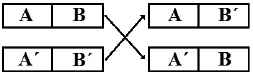
One-point recombination.
2.2.5. Two-point recombination
Similar to above but instead of a single cut-off point, two cut-off points are selected from each parent chromosome, which defines a sequence that is exchanged between parents to produce offspring (see Figure 2). With this operator, new blocks are generated, so it is more disruptive than the previous operator. It is recommended in21 not to use recombination operators for one and two points alone because they can generate premature convergence. However by combining them with mutation and transposition operators, thorough exploration of the feature space is achieved.
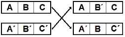
Two-point recombination.
3. Classification with discriminant functions
Discriminant functions are one of the schemes used in data mining for classification9. In a discriminant function, a subset of the attributes of a pattern is taken for classifying; the output is computed as a value that is the result of evaluating the function at these input attributes. Then, this value must be compared with a threshold (normally 0) to associate it with the corresponding initial pattern classification22 (see equation 1) where X is the input feature vector.
This classifier will consist of a list of discriminant functions where each function associates an output class. In the case of two classes, the classifier would be as in equation 2.
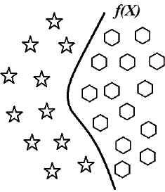
Characteristic space splitting by a discriminant function.
The multi-class problem can be resolved by using a one-vs-all approach23, where the n-class problem is transformed into n two-class problems. In this approach, the instances of each class are taken as positive instances and the rest as negative instances. On the other hand, a way to build the classifier would be to find a single discriminant function for each class. However, it has the disadvantage that in the real-world problems the features spaces are usually much more complex than Figure 3, given that one function is generally not able to classify all instances of a determined class properly. Thus, we need to find more than one function for each class: the proposed algorithm searches for discriminant functions to achieve a certain predefined level of coverage over all instances for each class; new functions are added to the solution only when they cover instances not covered by previous functions.
Once the discovery process of discriminant functions concludes, a decision list is generated, with the best functions at the top of the list. When a new instance is presented to this classifier to predict its class, the first function of the list is evaluated. If it returns a positive value, the class associated with this discriminant function is established. If it returns a non-positive value, then the evaluation passes on to the next discriminant function, and so on24. If no discriminant function returns a positive value, the most numerous class in the training set is returned as the default class, as shown in equation 3.
4. Multi-class with gene expression programming algorithm (MCGEP)
This classifier is based on a version of the steady-state algorithm with elitism defined in25 and it is a modified version of the inspiring algorithm proposed in19. In this algorithm, a list of non-redundant individuals is generated with respect to covered instances of the training collection, this process is repeated for each class. To achieve that, a token competition is performed, similar to one proposed by Wong and Leung in26.
The fitness of each individual is calculated by multiplying its previous fitness value with the rate between winning tokens and possible-to-win tokens. A token is an instance of the training collection. Covered instances are removed from the competition. Thus, redundant individuals obtain a low fitness score (zero if they cover the same instances covered by others previous individuals in the population). An individual with good initial fitness but with a low rate of new (not covered by others) won-tokens may finish the competition with low fitness, even with zero fitness, in the worst case. Before each competition, individuals token-winners are sorted according to their fitness.
4.1. Function set and terminal set
In MCGEP only basic arithmetic functions have been used to build the discriminant functions that form the final classifier as a decision list; the function set was formed by operations: * (multiplication), / (division), + (addition) and − (subtraction); in all cases these functions were established with arity equal to 2. For the moment, the algorithm has only been developed for numerical data sets; the intention is to make an implementation that works on numerical and non-numerical data sets for greater generality. So the terminals are the attributes of a data set or the constants that were initially defined in the algorithm configuration file. Each individual encodes one rule, representing a discriminant function and having a class as a consequent. The consequent represents the current class in each run of the algorithm, so the algorithm runs as many times as the number of existing classes.
4.2. Fitness function
This function (see equation 4) evaluates the fitness of each individual (rule or discriminant function) to be applied to the collection of training; this metric is similar to that used by Bojarczuk et al. in27 for a classification rule discovery system with genetic programming.
The third factor is a measure of the simplicity of an individual. This is included because the proposed algorithm does not necessarily produce simple individuals. Although they are limited by the maximum size defined by the GEP chromosome which is maxSize = 2 (headsize) + 1. The variable phenotSize in the equation 4 is the length (number of terminal and non-terminal elements) of the expression tree coded in the phenotype of an individual; this factor reaches its maximum unitary value when a phenotype is as simplest as possible (phenotype length equal to one). This factor was designed as a negative slope line and decreases to a minimum of 0.8 when length equals the maximum phenotype represented by the value: maxSize. Thus, the most complex individuals are penalized, although not forced to disappear, during the evolutionary process and fitness surface exploration almost obeys the parsimony principle: “the simplest is the best”. Thus, fitness function is defined (see equation 4) by multiplying the three factors and then taking values between 0 and 1.
4.3. General characteristics of MCGEP algorithm
To implement the MCGEP algorithm, we reviewed two excellent algorithms for rule discovering, namely Tan et al.19 and Zhou et al.20. In the Tan algorithm, individuals were encoded like in genetic programming. In Zhou, a GEP variant with a validity test was used. Finally, in MCGEP algorithm, we coded individuals exactly the same way as Ferreira10,21 defined them in his work, since it is a much simpler scheme. In the Tan algorithm, the well-known method ramped-half-and-half was used to generate the initial population. In Zhou, the initial population was generated completely randomly.
In MCGEP, we chose the criterion of random generation but kept the head and tail structure, thus avoiding the introduction of new parameters (and adjusting to Ferreira’s definitions). In Tan, only logical operations AND and NOT (normal disjunctive form) were used as function set. In Zhou arithmetic (*, +, −, /, sqrt) and logical (if x > 0 then y else z) operations were used as function set. Again, we used simplicity as the criterion for the MCGEP function set and only used four basic operators (*, +, −, /), all of them with arity = 2. For Tan, only nominal attributes were allowed, since all combinations of attribute-value were used as the terminal set. Zhou worked with numeric attributes (nominal binarization). For MCGEP, we used the same Zhou scheme (numerical or nominal binarization when needed).
In all cases, the classifier was constructed as a decision list. The Tan method used a threshold to avoid over-fitting. However in Zhou, the MDL (Minimal Description Length) principle was used, with a value W = 0.5. In our case, although we found Zhou’s approach with MDL very interesting, we used the threshold method, which is far simpler and provides very good results (scant over-fitting). On the other hand, as Bacardit30 poses in chapter 8 of his report, the W parameter setting becomes very sensitive product selection pressure of genetic algorithms. Making for high values a collapse of the final classifier into one with a single rule; for small values of the parameter, the classifier fails to eliminate over-fitting. Later, Bacardit states that it is no simple task to automatically adjust this parameter, so its inclusion in our algorithm is left for future implementations.
The Tan algorithm used a fitness function with the product of sensitivity and specificity. In Zhou, the product of rule consistency by completeness gain ratio (covered entities) was used. In our case, we modulated the products of sensitivity and specificity with a third factor (which prioritizes the simplicity of the rules). To control diversity, Tan used a token competition. In Zhou, the instances covered are progressively removed from the data set. In our case, we used the method that Tan employs in his algorithm to adjust the fitness of individuals, depending of the new instances covered. In this way, the algorithm tends to eliminate redundancy, while the more general rules are prioritized.
Table 1 shows a comparison of the basic characteristics of MCGEP and the two fundamental works that inspired its development: Tan and Zhou.
| Features | Tan 200219 | Zhou 200320 | MCGEP |
|---|---|---|---|
| Individual coding | GP | GEP (with validity test) | GEP |
| Initialization method | Ramped-half-and-half | Completely random | Random, but conserving head and tail structure |
| Function set | AND, NOT | *, +, −, /, sqrt, if-then | *, +, −, / |
| Terminal set | All combinations of attribute-value (nominal) | Numeric and nominal binarization | Numeric |
| Constants set | - | Constant list | Constant list |
| Kind of rules | Classifications rules | Discriminant Functions | Discriminant Functions |
| Kind of classifier | Decision list | Decision list | Decision list |
| Method to avoid overfitting | Support threshold | MDL | Support threshold |
| Fitness function | F = Sen * Esp | F = ConsistGain * Complet | F = Sen * Esp * Sim |
| Diversity control | Token Competition | - | Token Competition |
Comparative table.
4.4. Pseudo-code algorithm description
As shown in the line 4 of the pseudo-code (Algorithm 1), the evolutionary process begins by generating the initial population bset(0). This initial population evolves for several generations until the stop condition is reached -in our algorithm, that means until the maximum number of generations gmax is achieved (this parameter is defined in the algorithm configuration file) or an individual with fitness ≈ 1 obtained. In each generation, individuals are evaluated according to the performance function defined in 4.2 (see equation 4). Then a small elite percentage population is chosen, which is defined in the configuration file by the parameter elitistperc and saved in (cset) (see line 8 of pseudo-code). A selection of parents is performed on the remaining population, with two of tournament size, tournsize = 2 (see line 10); to select the parents (pset), the GEP genetic operators detailed in section 2.2 were applied one by one (see lines 11 to 15); thereafter, the offspring obtained (in rset) were evaluated (see line 16). Subsequently, a reproduction process where some individuals from the original bset population are randomly chosen with a low probability defined in the configuration file as copyprob = 0.1 and bound to the previously obtained elite population (cset) (see line 17); finally individuals: cset, eset and rset are joined in a unique population cset (initially eset is empty), as can be seen in lines 18 and 19. Then, a TokenCompetition on cset population is executed (see line 20), the competition returns a vector of rules that are then stored in eset which is a potential classifier for the current class, the eset rules were obtained from individuals who had a reason (CoveredTokens/TotalTokens) > thresholdsupport, then eset population is re-evaluated to prepare for the next generation (see line 21), in the line 22, the population is adjusted back to the original size defined by popsize. The whole process is repeated generation after generation from line 6 until it reaches the maximum number of generations, or an individual achieves a fitness very close to 1.0. If any of the above stop conditions is reached, all the elements of eset are added to the classifier and the algorithm starts with the next class, repeating the whole process from line 3 onwards.
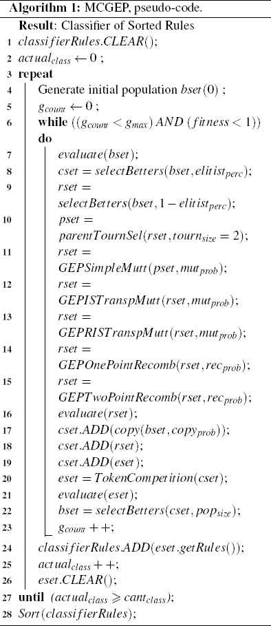
MCGEP, pseudo-code.
The class used for fitness calculation is assigned in each algorithm iteration as a rule consequent, assuming as positive instances those belonging to that class and as negative those belonging to other classes. The algorithm is repeated as many times as the number of existing classes in the training set. All the rules coded in eset individuals are added to classifier in each cycle. The list eset is reset each time; see line 26. At the end of the process, we sort all rules in the classifier according to the PPV value. In each sorting cycle, we add the PPV-best rule to the end of a list of rules and remove all the matching instances from the training set. We repeat this process until the training set is empty or no more rules for sorting (we initially used an empty list of rules and the full training set to calculate the first PPV-best rule). PPV is computed as PPV = tp/(tp + fp).
5. Empirical evaluation
This section presents the experimental methodology followed to evaluate the algorithms presented. The accuracy and the size of the models evolved by all algorithms involved in this work is compared. The competence of the MCGEP is compared with nine widely-known GP techniques for discovering classification rules that represent a large variety of learning paradigms. The methods used in the comparison are:
- 1.
- 2.
- 3.
- 4.
SLAVE36: genetic fuzzy-rule-based classifier that implements iterative rule learning with the search space reduction objective.
- 5.
- 6.
CORE40: in the co-evolutionary algorithm for rules discovery, each individual codifies a rule and the whole rule set is evolved simultaneously. Thus, rules should cooperate with each other to produce an optimal rule set jointly, and at the same time, the rule set is reduced by a token competition.
- 7.
Bojarczuk27: a hybrid Pittsburgh/Michigan approach, where an individual can contain multiple classification rules that predict the same class. An individual is in disjunctive normal form (DNF). An individual consists of a logical disjunction of rule antecedents, where each rule antecedent is a logical conjunction of conditions (attributevalue pairs). This is a genetic programming rule-based system.
- 8.
Falco41: Michigan-style genetic algorithm able to extract classification rules. Each rule is constituted by a logical combination of predicting attributes. It is a grammar guided genetic programming based system.
- 9.
Tan19: extends the tree representation of genetic programming to evolve multiple comprehensible IF-THEN classification rules in a Michigan-style. It employs a covering algorithm (token competition) inspired by the artificial immune system, where a memory vector is utilized to produce multiple rules, as well as to remove redundant rules. It is a grammar guided genetic programming-based system.
A more detailed explanation of each of the first six algorithms above can be found condensed in an excellent review18.
The following subsection, provides details of the real-world problems chosen for the experiments, the experimental tools and configurations parameters for each one, the experimental results and the statistical analysis applied to compare the results obtained.
5.1. Training sets
To evaluate the behavior of our classifier, twenty real-world data sets were chosen from KEEL*42 and UCI†43 repositories.
UCI is a well-known repository and KEEL is an open source Java software tool which empowers the user to assess the behavior of evolutionary learning and Soft Computing based techniques. In particular, KEEL-dataset includes the data set partitions in the KEEL format classified as: regression, clustering, multi-instance, imbalanced classification, multi-label classification and so on. To execute the experiments, the following data sets were used: Australian, Balance, Bupa, Cleveland, Contraceptive, Dermatology, Ecoli, Glass, Heart, Iris, Pima, Sonar, Texture, Thyroid, Wdbc, Wine, Wisconsin, Wpbc, Yeast and Zoo. In our experimental assessment, all examples with missing values were removed from the data sets. In total, we have eight binary problems, five three-class problems and seven problems between 5 and 11 class. A summary of the characteristics of these data sets can be seen in the Table 2.
| Id. | Data set | Instances | Attrib. | Class |
|---|---|---|---|---|
| aus | Australian | 690 | 14 | 2 |
| bal | Balance | 625 | 4 | 3 |
| bup | Bupa | 345 | 6 | 2 |
| cle | Cleveland | 297 | 13 | 5 |
| con | Contraceptive | 1473 | 9 | 3 |
| der | Dermatology | 358 | 34 | 6 |
| eco | Ecoli | 336 | 7 | 8 |
| gla | Glass | 214 | 9 | 7 |
| hea | Heart-s | 270 | 13 | 2 |
| iri | Iris | 150 | 4 | 3 |
| pim | Pima | 768 | 8 | 2 |
| son | Sonar | 208 | 60 | 2 |
| tex | Texture | 5500 | 40 | 11 |
| thy | Thyroid | 7200 | 21 | 3 |
| wdb | Wdbc | 569 | 30 | 2 |
| win | Wine | 178 | 13 | 3 |
| wis | Wisconsin | 683 | 9 | 2 |
| wpb | Wpbc | 194 | 32 | 2 |
| yea | Yeast | 1484 | 8 | 10 |
| zoo | Zoo | 101 | 17 | 7 |
Data set characteristics.
5.2. Experimental tools
We used the JCLEC‡ framework described in44; it is a software system for Evolutionary Computation (EC) research, developed in Java programming language.
It provides a high-level software framework to perform any kind of Evolutionary Algorithm (EA), providing support for genetic algorithms (binary, integer and real encoding), genetic programming (Koza’s style, strongly typed, and grammar based) and evolutionary programming. It has a module for classification, where the MCGEP algorithm described in Section 4 was implemented, GEP genetic operators of JCLEC were used. The evaluator was implemented in JCLEC with the fitness function described in section 4.2. Furthermore, to perform the simulations, a cluster with Multi-Core 12 × 2.4 GHz processors, 23.58 GB of RAM and Linux 2.6.32 as the operating system were used. The parameters used in the algorithm are summarized in Table 3. They were kept constant during the experiments. In our experiments, we used the chromosome size and constants list dependent on the characteristics of the problem. The list of constants is chosen depending on the range of attribute values (only in glass, heart-s, pima, wdbc and wine). The configuration files for MCGEP and complementary material of the experimental study can be consulted at the link§.
| Parameter | Value |
|---|---|
| Population Size (population-size) | 500 |
| Max of Generations (max-of-generations) | 100 |
| Tournament selector (tournament-size) | 2 |
| Copy probability (copy-prob) | 0.1 |
| Elite probability (elitist-prob) | 0.1 |
| Support (support) | 0.01 |
| Parameters (w1 ; w2) | (1 ; 2) |
| GEPSimpleMutator (mut-prob) | 0.15 |
| GEPISTranspositionMutator (mut-prob) | 0.10 |
| GEPRISTranspositionMutator (mut-prob) | 0.10 |
| GEPOnePointRecombinator (rec-prob) | 0.40 |
| GEPTwoPointsRecombinator (rec-prob) | 0.40 |
MCGEP sumary parameters.
How the size of the head in GEP is defined, remains an open issue10,45, so we adjusted this parameter through trial and error starting with values close to ten times the number of attributes of each data set. To achieve repeatability of the experiments, we show the configurations of each problem in Tables 3 and 4. The source codes and optimum configurations for UCS, GASSIST, HIDER, SLAVE, LOGIT-BOOST and CORE were based in KEEL46, its original authors and in the useful review paper18. We used the JCLEC implementation of the Bojarczuk, Falco and Tan algorithms, with the configurations recommended by the original authors19,27,41 respectively.
| Dataset | Headsize | Const. List |
|---|---|---|
| Australian | 140 | 1;0.5 |
| Balance | 25 | 1;0.5 |
| Bupa | 40 | 1;0.5 |
| Cleveland | 130 | 1;0.5 |
| Contraceptive | 90 | 1;0.5 |
| Dermatology | 340 | 1;0.5 |
| Ecoli | 70 | 1;0.5 |
| Glass | 100 | 1;0.5;5;50 |
| Heart-s | 150 | 1;0.5;5;50 |
| Iris | 40 | 1;0.5 |
| Pima | 60 | 1;0.5;10;400 |
| Sonar | 65 | 1;0.5 |
| Texture | 400 | 1;0.5 |
| Thyroid | 180 | 1;0.5 |
| Wdbc | 300 | 1;0.5;50;500 |
| Wine | 130 | 1;0.5;50;500 |
| Wisconsin | 90 | 1;0.5 |
| Wpbc | 80 | 1;0.5 |
| Yeast | 80 | 1;0.5 |
| Zoo | 170 | 1;0.5 |
MCGEP problem configuration.
5.3. Experimental results
We evaluated the performance of the models evolved by each learning system with the test accuracy metric (proportion of correct classifications over previously unseen examples) and number of rules of the models obtained in each case. We used a ten-fold cross validation procedure with 5 different random seeds over each data set. The average results for each collection are shown in Table 5, for accuracy and in Table 6 for number of rules. The last row in Tables 5 and 6 shows the average rank for each algorithm.
| Data set | MCGEP | UCS | GASSIST | HIDER | SLAVE | LOGIT-BOOST | CORE | Bojarczuk | Falco | Tan |
|---|---|---|---|---|---|---|---|---|---|---|
| aus | 85.57(2) | 84.12(6) | 86.43(1) | 81.65(8) | 70.29(10) | 83.59(7) | 78.67(9) | 85.51(3.5) | 85.51(3.5) | 84.58(5) |
| bal | 97.76(1) | 74.65(5) | 78.88(3) | 69.73(7) | 75.58(4) | 89.75(2) | 65.39(8) | 55.34(10) | 58.80(9) | 71.68(6) |
| bup | 69.34(1) | 65.12(3) | 61.86(5) | 63.33(4) | 58.21(8) | 69.28(2) | 57.98(9) | 55.76(10) | 58.98(6) | 58.23(7) |
| cle | 54.43(3) | 53.03(8) | 56.19(1) | 53.17(6) | 53.63(5) | 53.88(4) | 53.00(9) | 50.28(10) | 53.06(7) | 55.34(2) |
| con | 52.05(4) | 48.19(7) | 54.58(1) | 52.52(3) | 43.82(9) | 53.38(2) | 44.23(8) | 49.04(5) | 42.53(10) | 48.47(6) |
| der | 94.95(2) | 90.57(5) | 95.96(1) | 88.54(6) | 90.74(4) | 31.03(10) | 31.75(9) | 85.63(7) | 73.87(8) | 93.32(3) |
| eco | 72.11(7) | 79.30(3) | 77.23(4) | 75.74(5) | 83.95(2) | 84.54(1) | 66.57(9) | 65.49(10) | 70.31(8) | 72.22(6) |
| gla | 67.33(3) | 72.66(1) | 66.82(4) | 62.63(5) | 59.91(6) | 69.14(2) | 50.56(9) | 50.37(10) | 54.63(8) | 57.98(7) |
| hea | 81.70(1) | 77.78(5) | 79.78(2) | 75.19(7) | 78.59(3) | 78.22(4) | 68.44(10) | 70.00(9) | 70.74(8) | 76.81(6) |
| iri | 96.53(1) | 94.80(7) | 96.40(2) | 96.00(4.5) | 95.33(6) | 96.00(4.5) | 94.53(8.5) | 91.60(10) | 94.53(8.5) | 96.13(3) |
| pim | 74.05(3) | 71.78(9) | 73.88(4) | 74.29(2) | 73.84(5) | 75.40(1) | 72.56(7) | 71.44(10) | 73.48(6) | 72.07(8) |
| son | 74.38(2) | 66.84(7) | 76.10(1) | 50.78(10) | 70.98(5) | 54.88(8) | 53.38(9) | 72.00(4) | 73.26(3) | 68.49(6) |
| tex | 81.03(4) | 93.77(1) | 62.88(6) | 84.87(2) | 82.37(3) | 58.95(7) | 09.09(10) | 52.46(8) | 43.63(9) | 67.31(5) |
| thy | 94.85(1) | 92.29(8) | 94.79(2) | 93.96(3) | 93.03(5) | 93.56(4) | 92.58(7) | 77.92(10) | 92.84(6) | 88.76(9) |
| wdb | 94.55(2) | 94.73(1) | 93.78(4) | 85.17(9) | 91.38(6) | 93.85(3) | 65.59(10) | 89.07(7) | 89.04(8) | 93.05(5) |
| win | 95.03(3) | 96.16(2) | 93.90(4) | 79.98(10) | 92.80(5) | 97.07(1) | 84.58(7) | 83.18(8) | 80.58(9) | 91.44(6) |
| wis | 96.55(1) | 96.36(2) | 95.59(4) | 96.23(3) | 95.57(5) | 91.04(10) | 93.23(7) | 92.66(8) | 91.71(9) | 95.33(6) |
| wpb | 73.63(3) | 71.45(5) | 70.61(6) | 64.43(8) | 72.83(4) | 69.79(7) | 76.32(1) | 58.07(10) | 75.73(2) | 62.12(9) |
| yea | 52.33(5) | 55.38(3) | 55.21(4) | 55.79(2) | 49.06(6) | 58.86(1) | 35.86(9) | 42.49(7) | 35.00(10) | 36.60(8) |
| zoo | 95.62(3) | 94.71(5) | 92.84(7) | 95.67(2) | 96.50(1) | 45.58(10) | 88.07(8) | 93.29(6) | 83.98(9) | 95.00(4) |
| Rank | 2.60 | 4.65 | 3.30 | 5.33 | 5.10 | 4.53 | 8.18 | 8.13 | 7.35 | 5.85 |
Algorithm accuracy and rank over data sets.
| Data set | MCGEP | UCS | GASSIST | HIDER | SLAVE | LOGIT-BOOST | CORE | Bojarczuk | Falco | Tan |
|---|---|---|---|---|---|---|---|---|---|---|
| aus | 10.44 | 6355.30 | 7.36 | 13.96 | 7.72 | 50.00 | 6.68 | 2.00 | 2.00 | 13.62 |
| bal | 8.58 | 5406.76 | 8.84 | 5.00 | 22.64 | 50.00 | 4.44 | 4.44 | 3.00 | 18.94 |
| bup | 13.06 | 6074.14 | 7.60 | 6.52 | 5.94 | 50.00 | 3.96 | 2.04 | 2.00 | 18.60 |
| cle | 19.84 | 6366.20 | 6.88 | 23.58 | 37.40 | 50.00 | 6.56 | 5.56 | 5.00 | 25.48 |
| con | 24.92 | 6397.38 | 7.90 | 13.84 | 46.66 | 50.00 | 6.12 | 3.02 | 3.00 | 32.36 |
| der | 11.60 | 6162.16 | 6.66 | 10.74 | 10.96 | 50.00 | 1.00 | 6.72 | 6.00 | 11.60 |
| eco | 19.32 | 6154.64 | 6.04 | 12.54 | 13.06 | 50.00 | 6.40 | 9.64 | 8.00 | 25.22 |
| gla | 17.22 | 6294.60 | 5.34 | 25.00 | 15.74 | 50.00 | 6.24 | 7.84 | 7.02 | 20.98 |
| hea | 9.60 | 6300.64 | 6.52 | 9.08 | 7.60 | 50.00 | 7.68 | 2.00 | 2.00 | 15.50 |
| iri | 5.18 | 3184.18 | 4.08 | 4.00 | 3.00 | 50.00 | 3.28 | 3.96 | 3.00 | 6.04 |
| pim | 12.62 | 6359.64 | 8.26 | 12.28 | 10.04 | 50.00 | 4.86 | 2.00 | 2.76 | 19.10 |
| son | 13.04 | 6384.58 | 5.24 | 179.00 | 7.98 | 50.00 | 1.00 | 2.00 | 2.00 | 16.04 |
| tex | 25.96 | 6400.00 | 11.12 | 89.74 | 35.14 | 50.00 | 1.00 | 15.86 | 11.02 | 35.62 |
| thy | 7.40 | 6399.74 | 5.70 | 3.16 | 6.76 | 50.00 | 2.14 | 3.46 | 3.00 | 9.66 |
| wdb | 6.74 | 6351.00 | 5.24 | 99.20 | 5.32 | 50.00 | 2.56 | 2.00 | 2.00 | 9.20 |
| win | 7.46 | 6326.84 | 4.24 | 30.82 | 3.96 | 50.00 | 3.76 | 3.00 | 3.00 | 9.20 |
| wis | 4.56 | 5743.26 | 4.18 | 3.10 | 6.08 | 50.00 | 6.40 | 2.00 | 2.00 | 6.88 |
| wpb | 12.34 | 6359.62 | 5.26 | 131.46 | 9.90 | 50.00 | 1.38 | 2.00 | 2.00 | 18.42 |
| yea | 45.62 | 6397.56 | 7.06 | 48.88 | 23.68 | 50.00 | 5.46 | 12.08 | 10.00 | 51.66 |
| zoo | 7.54 | 5822.30 | 7.10 | 7.60 | 7.30 | 50.00 | 7.74 | 9.08 | 7.00 | 8.40 |
| Rank | 6.08 | 10.00 | 3.75 | 6.25 | 5.28 | 8.75 | 2.73 | 2.90 | 1.80 | 7.48 |
Number of rules in models obtained over data sets.
5.4. Statistical analysis
We followed the recommendations pointed out by Demšar47 to perform the statistical analysis of the results. As he suggests, we used non-parametric statistical tests to compare the accuracies and sizes of the models built by the different learning systems. To compare multiple learning methods, we first applied a multi-comparison statistical procedure to test the null hypothesis that all learning algorithms obtain the same results on average. Specifically, we used Friedman’s test. The Friedman test rejected the null hypothesis, so post-hoc Bonferroni-Dunn tests were applied.
According to the results obtained (see Tables 5 and 6) we statistically analyzed the results to detect significant differences between the accuracy and the size of the models evolved by the different learning methods.
The multi-comparison Friedman’s test rejected the null hypotheses that (i) all the systems performed the same on average with p = 4.37 × 10⁻¹¹, (ii) the number of rules in the models was equivalent on average with p = 7.28 × 10⁻¹¹. Afterwards, we applied the post-hoc Bonferroni-Dunn test using KEEL tools to detect (i) which learning algorithm performed equivalently to the best-ranked method (MCGEP) according to the test accuracy metric; (ii) which methods evolved models whose number of rules were equivalent to the best ranked method (Falco) according to the model size. Using α = 0.10 in equation 5 with k, number of algorithms, qα = 2.539 and N, number of data sets, a critical difference of 2.4309 is obtained.
Figure 4 shows the results of this Bonferroni-Dunn test, comparing all systems in terms of both accuracy and the number of rules in the model. The major advantage of this test is that it seems to be easier to visualize, because it uses the same critical difference for all comparisons47.
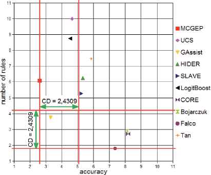
Critical difference comparison of accuracy and number of rules.
To check the results, we also applied the Holm’s step-up and step-down procedure sequentially to test the hypotheses ordered by their significance. The last one is more powerful than the previous Bonferroni Dunn single-step and it makes no additional assumptions about the hypotheses tested47. As can be seen in Table 7, accuracy via Holm’s test with α = 0.05 detect the same significant differences between MCGEP and SLAVE, HIDER, Tan, Falco, Bojarczuk and CORE as Bonferroni-Dunn. Holm’s at α = 0.05 does not detect significant differences among MCGEP and GASSIST, LOGIT-BOOST and UCS.
| i | algorithm | z = (R0 − Ri)/SE | p | Holm/Hochberg/Hommel |
|---|---|---|---|---|
| 9 | CORE | 5.8229 | 5.7836E-9 | 0.0056 |
| 8 | Bojarczuk | 5.7707 | 7.8955E-9 | 0.0063 |
| 7 | Falco | 4.9612 | 7.0054E-7 | 0.0071 |
| 6 | Tan | 3.3945 | 6.8750E-4 | 0.0083 |
| 5 | HIDER | 2.8462 | 0.0044 | 0.0100 |
| 4 | SLAVE | 2.6112 | 0.0090 | 0.0125 |
| 3 | UCS | 2.1412 | 0.0323 | 0.0167 |
| 2 | LOGIT-BOOST | 2.0106 | 0.0444 | 0.0250 |
| 1 | GASSIST | 0.7311 | 0.4647 | 0.0500 |
| /// | MCGEP | Control algorithm | /// | /// |
Holm / Hochberg Table for α = 0.05
In general, as the Bonferroni-Dunn test shows, the GASSIST method is the most balanced of all the alternative methods analyzed in this work. It also highlights the need to improve the MCGEP method proposed by this paper in regard to the size of the generated models. In the accuracy metric, MCGEP outperformed GASSIST, although the difference is not significant from the point of view of the statistical tests applied (Holm tests, α = 0.05). Taking both criteria (accuracy and model size) at the same time Tan, HIDER and SLAVE are the worst algorithms -see Figure 4. Falco, Bojarzuck and CORE behave well on the size of the generated models, however, they have a mediocre performance in accuracy. UCS and LOGIT-BOOST perform very well in terms of accuracy; in contrast, their performance is worse when attempting to obtain compact models.
As stated above, in statistical terms, when accuracy alone is taken into account, no significant differences were found between MCGEP, GASSIST, LOGIT-BOOST and UCS, although we can make some judgments about the performance of the algorithms in some application scenarios, for example, with variations in the number of classes and in the number of attributes in data sets. Nevertheless, it does not seem necessary to evaluate the variations in the number of instances of data sets.
The comparison was based on information from the individual ranking presented in Table 5. We divided the algorithms into three new ranks, High, Middle (Mid.) and Low. To do so, we attempted to make an equitable division by leaving the same number of ranks in each division and leaving the remaining elements in the Mid. division. For the number of classes, we make the division whenever possible in such a way that it had the same number of data sets in each division; we obtained the following data sets cases: (2) binary; (3–5) between 3 and 5 classes and (6–11) between 6 and 11 classes. For the number of attributes, we applied the same process but also trying to maximize the distances between one range and other. Attribute ranges (4–9), (13–21) and (30–60) were derived from these divisions and individual ranking taken from Table 5. Tables 8 and 9 have been created to provide better visualization of the count for classes and attributes respectively.
| Algorithm rank | MCGEP | |||
| Low | (8–10) | 0 | 0 | 0 |
| Mid. | (4–7) | 0 | 1 | 3 |
| High | (1–3) | 8 | 5 | 3 |
| Number of class ↦ | (2) | (3–5) | (6–11) | |
| Algorithm rank | GASSIST | |||
| Low | (8–10) | 0 | 0 | 0 |
| Mid. | (4–7) | 5 | 1 | 5 |
| High | (1–3) | 3 | 5 | 1 |
| Number of class ↦ | (2) | (3–5) | (6–11) | |
| Algorithm rank | LOGIT-BOOST | |||
| Low | 8–10 | 2 | 0 | 2 |
| Mid. | 4–7 | 3 | 3 | 1 |
| High | 1–3 | 3 | 3 | 3 |
| Number of class ↦ | (2) | (3–5) | (6–11) | |
| Algorithm rank | UCS | |||
| Low | 8–10 | 1 | 2 | 0 |
| Mid. | 4–7 | 4 | 3 | 2 |
| High | 1–3 | 3 | 1 | 4 |
| Number of class ↦ | (2) | (3–5) | (6–11) | |
Class distribution count in rank achieved by each algorithm. (2) means binary data sets, (3–5) means 3 to 5 class data sets. (6–11) means 6 to 11 class data sets. Algorithm rank High (1–3) mean algorithms that reach a high rank 1, 2 or 3, and so on.
| Algorithm rank | MCGEP | |||
| Low | (8–10) | 0 | 0 | 0 |
| Mid. | (4–7) | 3 | 0 | 1 |
| High | (1–3) | 6 | 6 | 4 |
| Number of class ↦ | (4–9) | (13–21) | (30–60) | |
| Algorithm rank | GASSIST | |||
| Low | (8–10) | 0 | 0 | 0 |
| Mid. | (4–7) | 6 | 2 | 3 |
| High | (1–3) | 3 | 4 | 2 |
| Number of class ↦ | (4–9) | (13–21) | (30–60) | |
| Algorithm rank | LOGIT-BOOST | |||
| Low | 8–10 | 1 | 1 | 2 |
| Mid. | 4–7 | 1 | 4 | 2 |
| High | 1–3 | 7 | 1 | 1 |
| Number of class ↦ | (4–9) | (13–21) | (30–60) | |
| Algorithm rank | UCS | |||
| Low | 8–10 | 1 | 2 | 0 |
| Mid. | 4–7 | 3 | 3 | 3 |
| High | 1–3 | 5 | 1 | 2 |
| Number of class ↦ | (4–9) | (13–21) | (30–60) | |
Attribute distribution counts in rank achieved by each algorithm. (4–9) means data sets with 4 to 9 attributes, (13–21) means data sets with 13 to 21 attributes. (30–60) means data sets with 30 to 60 attributes. Algorithm rank High (1–3) means algorithms that reach a high rank 1, 2 or 3, and so on.
As shown in Table 8, MCGEP algorithm achieves a high level (first three places in the ranking) in 16 of the 20 data sets. In the binary data sets, it achieves the best performance, since it is ranked among the top three in all of them. In the twenty data sets evaluated, this algorithm has no Low performances. In half of the data sets between 7 and 10 classes, its performance is High, while it also achieves Mid. performance in the other half.
The GASSIST algorithm (second in the overall-ranking) achieves High performance in almost half of the data sets, however in the binary data sets, its performance is basically Mid. It attains the performance of MCGEP in data sets between 3 and 7 classes.Like the previous algorithm, GASSIST also has no Low performance in data sets. The performance of the LOGIT-BOOST algorithm is High in almost half of the data sets, however in the binary and in some many-classes (meaning in our work between 7 and 11 classes) data sets, have a Low performance. Finally, UCS excels over the other four algorithms in many-classes data sets. In this many-classes data sets, its performance was between Mid. and High.
When a similar analysis is performed but this time considering the distribution of attributes (see Table 9), we note that MCGEP excels in data sets of many-attributes (read for this work between 30 and 60 attributes). In four of the five data sets, it achieves High performance and in the fifth a Mid. performance.
In contrast, the LOGIT-BOOST algorithm has the worst performance in data sets with many-attributes. In the case of MCGEP, its performance is High for attributes between 13 and 21, and often it has High performance with few-attributes (4 to 9). The LOGIT-BOOST algorithm only slightly excels in the case of few-attributes, where most of the time it is the algorithm with High performance.
In summary, the MCGEP algorithm can be said to have good performance in data sets with a variable number of attributes. In consonance with the adjustments made to headsize parameter, this indicates that we used a correct heuristic to adjust this parameter (headsize ≈ 10 * attributesnumber). Nevertheless, we noted a slight reduction in the performance of this algorithm with many-classes data sets, this may be due mainly to the one-vs-all (OVA) approach used. It is well-known that imbalanced training data sets are produced when instances from a single class are compared to all other instances48. MCGEP is not completely ready to deal with this undesirable effect. For that reason, two future lines of work have been identified. The first, an implementation of the one-vs-one (OVO) approach and the second, to provide in-built support for this imbalance issue.
XCS and GASSIST were stated in the review17 as being “the two most outstanding learners in the GBML history”. On the other hand, Orriols-Puig et al.18 presented UCS (the evolution of XCS) as the learning algorithm that resulted in the most accurate models on average. Also Orriols-Puig et al.18 conclude that GASSIST yielded competitive results in terms of accuracy. We found GASSIST, LOGIT-BOOST and UCS to provide very similar results in their behavior during our assessment of MCGEP. Therefore we feel it is not fitting to make pairwise comparisons when we only tested whether a newly proposed method is better than existing ones47.
6. Conclusions and further work
In this paper, we tested and statistically validated the competitiveness of an algorithm for discovering classification rules with gene expression programming (MCGEP) in particular in terms of the accuracy metric. It was built by taking elements from several other inspiring works described in current literature. The product of sensibility, specificity and simplicity was taken from27 as a function of fitness, while Token Competition and the vision of creating vectors with candidate solutions came from19. The vector of candidate solutions was used to drive the evolutionary process by re-calling the best rules from the previous generation to the next generation, like the human immunology system remembers previous pathological conditions. The gene expression programming paradigm proposed by Ferreira in10 with the adjustments described in detail in21 was used in the coding of individuals, which ensures intrinsic efficiency in the evolutionary process. Twenty data sets (numerics or binarized-nominals) were adopted from KEEL and UCI projects. To validate the competitiveness of MCGEP, a comparison was made against nine well known algorithms. The experimental results achieved on twenty benchmark real-world data sets detailed in section 6 show that our approach is significantly better with respect to the accuracy metric than some state-of-the-art genetic rule-based algorithms (i.e., SLAVE, HIDER, Tan, Falco, Bojarczuk and CORE) and not significantly worse than other better algorithms (i.e., GASSIST, LOGIT-BOOST and UCS). Thus, the competitiveness of the GEP approach for discovering classification rules was empirically demonstrated. On the other hand, GASSIST was the most balanced method of all the others assessed in this work. Throughout this study, we have identified the strengths but also the weaknesses of the approach used and thus a great deal of future work remains to be carried out: the possibility of using nominal attributes; the inclusion of the principle of minimum description length (MDL) as used by Zhou et al20 to reduce the slight over-fitting that exists in some cases; the treatment of un-balanced data or the implementation of OVO variant to replace the current OVA variant; the possibility of imposing different costs on misclassification. A method for adjusting the parameters w1 and w2 needs to be researched, as does the implementation of multi-objective version, in order to perform searches of candidate solutions over the Pareto front. Furthermore, we need to make improvements in reducing the number of models generated because it was clearly seen to be one of the weak points of this work.
Acknowledgements
“This project was funded by the Deanship of Scientific Research (DSR), King Abdulaziz University, Jeddah, under grant No. (2-611-35/HiCi) and the Spanish Ministry of Economy and Competitiveness and FEDER funds under grant No. TIN2014-55252-P. The authors therefore express their sincerest gratitude for such technical and financial support”.
Footnotes
References
Cite this article
TY  - JOUR
AU  - Alain Guerrero-Enamorado
AU  - Carlos Morell
AU  - Amin Y. Noaman
AU  - Sebastián Ventura
PY  - 2016
DA  - 2016/04/01
TI  - An algorithm evaluation for discovering classification rules with gene expression programming
JO  - International Journal of Computational Intelligence Systems
SP  - 263
EP  - 280
VL  - 9
IS  - 2
SN  - 1875-6883
UR  - https://doi.org/10.1080/18756891.2016.1150000
DO  - 10.1080/18756891.2016.1150000
ID  - Guerrero-Enamorado2016
ER  -