
Control of a chain pendulum: A fuzzy logic approach
- DOI
- 10.1080/18756891.2016.1150001How to use a DOI?
- Keywords
- Intelligent control; fuzzy logic; rotary inverted pendulum; stabilization; Takagi-Sugeno model; region of attraction; robustness
- Abstract
In this paper we present a real application of computational intelligence. Fuzzy control of a non-linear rotary chain pendulum is proposed and implemented on real prototypes. The final aim is to obtain a larger region of attraction for the stabilization of this complex system, that is, a more robust controller. As it is well-known, fuzzy logic exploits the tolerance for imprecision, uncertainty and partial truth to achieve tractability, robustness and low solution cost when dealing with complex systems. In this case, the control strategy is based on a Takagi-Sugeno fuzzy model of the strongly non-linear multivariable system. Simulation and experimental results on the real plant have been obtained and tested in a rotary inverted pendulum and in a double rotary inverted pendulum. They have been compared to other feedback control strategies such as Full State Feedback or Linear Quadratic Regulator with encouraging results. Fuzzy control allows to enlarge the stability region of control. Indeed, the region of attraction and therefore the stabilization has been enlarged up to over 17% for the real system.
- Copyright
- © 2016. the authors. Co-published by Atlantis Press and Taylor & Francis
- Open Access
- This is an open access article under the CC BY-NC license (http://creativecommons.org/licences/by-nc/4.0/).
1. Introduction
In recent times, fuzzy control has been one of the most active areas in control design and computational intelligence. As it is well-known, fuzzy logic exploits the tolerance for imprecision, uncertainty and partial truth to achieve tractability, robustness and low solution cost. Besides, this intelligent control approach shows good robustness properties against model uncertainties and external disturbances. Up to now, fuzzy control has been successfully applied to a wide range of applications because of these properties 1.
In this regard, inverted pendulum systems have been revealed as the basis of many real applications. For example, the flight of rockets is closely related to the behavior of the rotary inverted pendulum. The control of the position of the rocket respect to the direction that engines are firing is analogous to the control of the rotary inverted pendulum. Other known applications are the self-balancing unicycle and the two-wheeled inverted pendulum. The first one is an electrical vehicle that can be approximated to a non-linear control system similar to a two-dimensional inverted pendulum with a unicycle cart at its base. The second one has been popularized principally trough the commercial variant Segway, which consists of a pendulum attached to a base platform that has a wheel at each side.
In addition, the inverted pendulum is implicitly present in systems like robot’s limbs or some elements of satellites. Moreover, the techniques derived for the inverted pendulum have been useful for the control of other unstable systems, such as aircraft of difficult manual control.
Indeed, the control of pendulum models has been chosen as a benchmark for years because it is considered a challenging testing ground for non-linear dynamical models and control theory. The complexity of these models, and hence of the controller, depends on the number of links and the degrees of freedom of each of them. There exist many types of inverted pendulums. The Furuta pendulum 2 has been used by some authors 3,4,5. Generalized models such as 3D pendulums have also been more recently developed 6. Variations as the pendubot 7 and the acrobot 8 have been also studied.
The main difference of the rotary inverted pendulum with other structures is produced by the rotation of the arm. Due to it, additional complexities are added in form of Coriolis forces and centrifugal torques. This provides not only a more involved mathematical model but also interesting behaviors to study. The strong non-linearity of the multi-output system and, therefore, the difficulty and complexity of the control design, has made the inverted pendulums an interesting case of study that has been used as a benchmark to test and compare different control strategies, such as in 9.
Typically, the control of a single 2D inverted pendulum consists of two different steps: The swinging-up motion and the stabilization control. The first one balances the pendulum to bring it closer to the upright position, i.e., the unstable equilibrium point (α = 0° in Figure 1). The second one stabilizes the pendulum to this point, where the system can be approximated to a linear system and conventional control laws such as Full State Feedback (FSF) or Linear Quadratic Regulator (LQR) can be used.
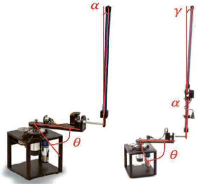
Prototype of the rotary inverted pendulum (left), and prototype of the double rotary inverted pendulum (right), by Quanser.
A similar strategy can be applied to control the double inverted pendulum: The two-step approach is followed by the link at the bottom (swing up and stabilization). Once this goal is achieved, the same two steps are repeated with the link at the top, but maintaining the control of the one at the bottom. In the case of the double pendulum on a cart, several swing-up strategies have been developed 10,11,12. However, for the double rotary inverted pendulum, as far as we know, the contributions found in the literature can be reduced to 13, where the swing-up control is only feasible for rotary double pendulums with particular characteristics.
In addition, the stabilization of analytic controllers only works well in a small neighborhood around the equilibrium, so the swing-up should be very precise. Naturally, the difficulty of this problem increases with the number of links. For this reason, it is interesting to search for new stabilization control strategies even when the initial conditions are far from the unstable equilibrium point and for a larger number of links.
In this regard, intelligent controllers can be a good approach 1,14. Both heuristic-based fuzzy control15 and model-based fuzzy control, such as Takagi-Sugeno fuzzy model 16, have been applied to many underactuated mechanical systems 17 . 18 stabilizes a quadruple inverted pendulum using a variable universe fuzzy controller. The tracking control is achieved in 19. Systems such as the two-wheel inverted pendulum 20 or the dual axis pendulums21 have been studied from this perspective.
Specifically, the control of the rotary inverted pendulum has been analyzed by several authors in the last years producing different control strategies, as for example fuzzy cascade control 22,23, evolutionary algorithms 24 , adaptive control 25 or the control based on an Takagi-Sugeno models 26,27. Other intelligent techniques such as neural networks have been widely applied to the identification of non-linear system, and therefore, the inverted pendulum in general and the rotary one have been chosen as a prime example 28,29. However, general rotary chains of pendulums have not been considered in the literature due to the complicated equations of motion which govern them.
The Takagi-Sugeno fuzzy model allows to approximate a nonlinear system to a combination of several linear systems in the corresponding fuzzy regions in the state space 15. The design of a linear controller for each linear subsystem produces a parallel distributed controller for the whole system 30. Model-based fuzzy control methods have the advantages of guaranteeing stability and robustness of the closed-loop system and, at the same time, producing desirable transient performance 31. In addition, the Takagi-Sugeno fuzzy model provides a larger read-ability than other approaches, such as neural networks.
In this paper, we show that the rotary chain pendulum can be modeled by Euler-Lagrange equations and a stabilization control can then be designed for the chain. A Takagi-Sugeno fuzzy model is developed to obtain a more robust feedback gain. Therefore, the main goal of this paper is the design of an intelligent control strategy that maximizes the region of attraction of the stabilization control of a rotary chain pendulum by means of a Takagi-Sugeno fuzzy model. As far as we know, there is no reference in the literature that proposes a controller of this type for an undetermined rotary chain. The designed control has been showed to provide larger regions of attraction and therefore more robust stabilization.
The paper is divided into 6 sections. In Section 2, the dynamics of the rotary chain pendulum and how to obtain a model from the Lagrangian of the system are explained. In Section 3, three different control methods (FSF, LQR and Takagi-Sugeno fuzzy) are described. Section 4 presents the two cases of study (simple and double rotary inverted pendulum). In Section 5, the results of applying the different control strategies to the two chain pendulum prototypes are shown and discussed. Section 6 gives the main conclusions of the paper.
2. Model of the rotary chain pendulum
In this section the theoretical model of the rotary chain pendulum is described using Lagrangian Mechanics. A rotary chain pendulum is a serial connection of n ⩾ 1 rigid links, connected by some joints and attached to a rigid arm which can rotate in a horizontal plane, perpendicular to the pendulums. It is an underactuated system because the n pendulums should be controlled only with the torque (τ) applied to the rotary arm. This rotating movement introduces Coriolis forces into the dynamics, making the analysis more complicated than if the system is a chain pendulum on a cart. The state of the system can be uniquely defined by a vector of generalized variables:
2.1. The Lagrangian
First of all, the Lagrange function or Lagrangian (L) is defined to apply the Euler-Lagrange method and to determine the equations of motion. The Lagrangian is defined as the difference between the kinetic energy (T) and the potential energy (V) of the system:
For the potential energy, let us consider the zero potential energy plane as the plane of the rotary arm. Then,
2.2. Equations of motion
The equations of motion of inverted pendulums can be derived from the Euler-Lagrange method using the Euler-Lagrange equation over the Lagrangian.
The equations of motion can be summarized as follows:
3. Control algorithms
While the stabilization control of the inverted pendulum has been extensively studied, it has not been generalized for any number of links. In this paper, we compare two classical analytic controllers with an intelligent controller designed to optimize the region of attraction using a Takagi-Sugeno fuzzy model. The following subsections describe the general form of the three controllers for a chain pendulum of n links.
3.1. Linear Controllers
In the state space, the equations of motion (5)–(6) can be linearized using a first order Taylor approach at point x0 = 0:
Knowing the desired poles from the specifications of the plant, the feedback gain is straightforward obtained applying pole placement techniques.
In the same way, a Linear Quadratic Regulator (LQR) can be implemented. LQR technique is an optimal control technique which consists in minimizing the cost function
We follow the criterion given by the Bryson’s rules in the choice of Q and R:
Even though the nonlinear system is locally stabilizable in theory, it can be easily deduced that the region of attraction can be very small when the number of links increases. We will show that a Takagi-Sugeno fuzzy controller can be implemented to enlarge the region of attraction. This results in a more robust control in the experimental plant.
3.2. Non-linear control based on Takagi-Sugeno fuzzy model
The fuzzy model proposed is described by means of a succession of IF-THEN rules, each of them expresses the local dynamic of a linear system. The output of the fuzzy model for any x is
The first step is to choose the nonlinearities of the system as p premise variables zp(t). Since the number of rules in the fuzzy model is determined by rM = 2pM, the following change of variables is proposed:
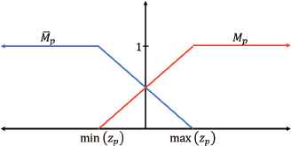
Example of membership function of variable zp.
Moreover, it is clear that,
Thus, the rules can be established and A, B and K matrices with constant elements are obtained. The fuzzy technique is applied to obtain a set of linear systems and their corresponding feedback gains following the rules:
Rule 1: IF z1 is ... Rule rM: IF z1 is M1 and ... zpM is MpM THEN ẋ(t) = ArMx(t) + BrMu(t) with u(t) = −KrMx(t).
As a result, Ki is obtained through LQR techniques. Finally, after a defuzzification process, the gain K applied to the non-linear system is computed as
Naturally, the number of rules grows up exponentially with the number of links. However, since the computation is performed offline, the resulting controller can be implemented on real systems with fast and/or unstable dynamics, such as pendulum chains, without worrying about the timing issue. In spite of that, even when the stability is guaranteed in the theoretical result, the region of attraction can be very small when the number of links is high. In fact, when n tends to infinity the control of the chain can be seen as an attempt to maintain vertical a rod moving only one of its ends. For this reason, the practical control of a chain of more than a few links can be unrealizable.
3.2.1. Stability criterion
The stability of the fuzzy closed-loop system is well developed. The globally asymptotically stability of the system (13) can be guaranteed with the following theorem 33:
Theorem:
The equilibrium of the continuous fuzzy control system described by (13) is globally asymptotically stable if there exists a common positive definite matrix P such that,
Proof.
The proof of the theorem can be found in 33.
4. Cases of study
The developed models and control strategies have been implemented in two cases of study: the rotary inverted pendulum and the double rotary inverted pendulum.
4.1. Rotary inverted pendulum
The system is shown in Figure 1 (left), where θ is the angle that the rotary arm forms with the X axis and α is the angle that the pendulum forms with the vertical axis. Then, the generalized coordinates of system,
According to the criterion proposed in Subsection 3.2, the following change of variables is done:
4.1.1. Control design for the rotary inverted pendulum
For the Full State Feedback control, we linearize (19)–(20) at
We apply Bryson’s rules to obtain the weight matrices of the LQR control:
Finally, we compute the fuzzy feedback (FZ) gain. By observing the mechanical parameters of the system, we have chosen max(z1) = max(z2) = 1, min(z1) = 0.9003, min(z2) = 0.7071, max(z3) = −min(z3) = 6, max(z4) = −min(z4) = 4.2426. These are the values that define the membership functions (Figure 2).
As an example of use, let us compute explicitly A1, B1 and K1. First, the values of the premise variables for the rule 1 are computed using (15)–(16):
Finally, by means of the defuzzification process (17), the fuzzy feedback gain is computed as
4.2. Double rotary inverted pendulum
The double rotary inverted pendulum consists of two links attached to a rotary arm (Figure 1, right). Again θ is the angle that the rotary arm forms with the X axis, α is the angle that the link at the bottom forms with the vertical axis and γ the angle of the link at the top. The generalized coordinates of system
4.2.1. Control design for the double rotary inverted pendulum
We can apply the LQR control of Subsection 3.1 to the linearized equations (21)–(22). The weight matrices are obtained from Bryson’s rules:
For the fuzzy control, the 12 premise variables are now:
5. Simulation and experimental results and discussion
In order to test and compare these controllers, the model described in Section 2 has been simulated following 26. The different strategies have been implemented using the rotary inverted pendulum of Figure 1 (left) and the double chain pendulum of Figure 1 (right), and compared.
The experimental setup of the rotary inverted pendulum 34,35 is showed in Figure 3. The power amplifier Quanser VoltPAQ transmits the voltage to the servo motor Quanser SRV02 which allows to actuate on the rotary arm. The measurements of the angles are sent to the computer through the data acquisition board Quanser Q8-USB. The applied controller running in the computer returns the input voltage that the power amplifier should give.

Scheme of the connection between the plant and the controller.
5.1. Results for the rotary inverted pendulum
First, the rotary inverted pendulum has been controlled using the three strategies presented in Section 4.1. In Figure 4 the simulation of the nonlinear model developed in Section 2 is depicted. First, a swing-up strategy based on the energy is used following the work of 3. Then the pendulum is stabilized using the three proposed techniques. In this way, we carry out fair comparison because the initial state should typically be the stable equilibrium position. We obtain that the maximum values of α that allow the stabilization are 37.2°, 40.1° and 51.6° for the FSF control, the LQR regulator and the fuzzy controller, respectively.
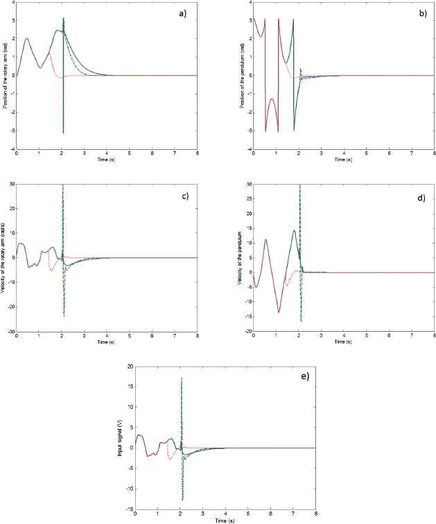
Simulation of the states and input signal for the three stabilization control strategies: a) Position of the rotary arm (rad), b) position of the pendulum (rad), c) velocity of the rotary arm (rad/s), d) velocity of the pendulum (rad/s), e) input signal (V). FSF control with switch at α = 37.2° (dashed green), LQR control with switch at α = 40.1° (solid blue), fuzzy control with switch at α = 51.6° (dotted red).
In the first part of the simulation (Figure 4), the lines are overlapped until we switch on the stabilization control because the swing-up control is the same, as we said. Because of the larger region of attraction of the fuzzy control (dotted red), the number of swings is reduced and, in consequence, the pendulum is stabilized faster. It can be observed that the FSF control (dashed green line) suffers a great disturbance when it comes into action due to the effort to reach its maximum region of attraction. On the contrary, the LQR (solid blue) and fuzzy control (dotted red) keep the system stable even when the region of attraction is larger.
The three control strategies designed in Section 3 have been tested on a real inverted pendulum system. Figure 5 illustrates the evolution of θ,
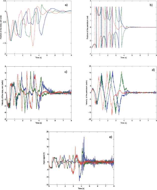
States and input signal in the experimental plant for the three stabilization control strategies: a) Position of the rotary arm (rad), b) position of the pendulum (rad), c) velocity of the rotary arm (rad/s), d) velocity of the pendulum (rad/s), e) input signal (V). FSF control with switch at α = 31.5° (dashed green), LQR control with switch at α = 34.3° (solid blue), fuzzy control with switch at α = 40.2° (dotted red).
If these results are compared with the simulation ones, we observe that the region of attraction results more conservative in the experimental plant. However, the control based on the Takagi-Sugeno model still provides larger region of attraction than the other controllers.
In addition, the settling time and the average steady state error are similar to the FSF and the LQR controllers, only the maximum overshoot is larger because of the need of a bigger thrust. Table 1 summarizes the results obtained with the three controllers in terms of the system response.
| FSF | LQR | Fuzzy | |
|---|---|---|---|
| Settling time (s) | 0.28 | 0.33 | 0.29 |
| Overshoot (rad) | 0.18 | 0.22 | 0.35 |
| Av. Steady state error (%) | 0.008 | 0.012 | 0.009 |
System response characteristics for the implemented controllers in the real rotary inverted pendulum.
5.2. Results for the double rotary inverted pendulum
The Takagi-Sugeno fuzzy model of the double rotary inverted pendulum (21)–(23) has been simulated.
The results of the system response for the LQR (dashed green) and fuzzy (dotted red) control strategies are presented in Figure 6. The maximum initial α for the LQR control is 14.5° and for the control based on the Takagi-Sugeno fuzzy model is 17.1°. In Figures 6.a and 6.c we can observe how the rotary arm recovers the reference position faster with the fuzzy control. However, the resulting overshoot in position and velocity of the pendulum (Figures 6.b and 6.f) are larger. The input signal (Figure 6.g) of both controllers is similar but the region of attraction increases 17.3% with the fuzzy control respect to the LQR control. This is a very good result for the robustness of the system.
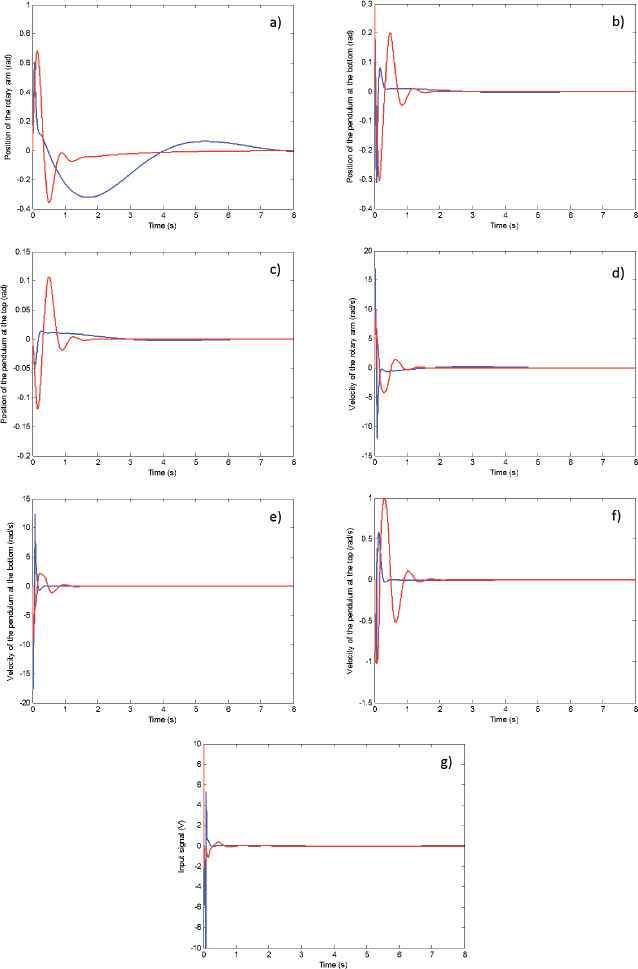
States and input signal in the stabilization of the double rotary inverted pendulum: a) Position of the rotary arm (rad), b) position of the bottom pendulum (rad), c) position of the top pendulum (rad), d) velocity of the rotary arm (rad/s), e) velocity of the bottom pendulum (rad/s), f) velocity of the top pendulum (rad/s), g) input signal (V). LQR control with initial α = 14.5° (blue) and fuzzy control with initial α = 17.1° (red).
6. Conclusions
In this paper we have presented a general form of the equations of motion of a rotary chain pendulum and the design of an intelligent controller based on a Takagi-Sugeno fuzzy model, which enlarges the region of attraction of the stabilization control of the chain pendulum.
This design has been applied to the rotary inverted pendulum and to the double rotary inverted pendulum, and compared to other feedback control strategies such as FSF and LQR.
From the experimental results with the real plant of the inverted pendulum, we can conclude that the region of attraction of the fuzzy model (40.2°) is considerably larger than with the FSF control (31.5°) or with the LQR control (34.3°). Specifically, it provides an improvement of 27.6% and 17.2%, respectively. These experimental results has been compared with the simulation ones, in which a larger region of attraction had been predicted for the fuzzy controller as well.
The fuzzy control has been also implemented in the double rotary inverted pendulum enlarging the region of attraction in 17.3%.
These results present a great applicability if we deal with very non-linear systems, where the region of attraction of classical controllers is not enough. For this reason, the application of fuzzy logic can be a way of making easier the swing-up control in complex inverted pendulum type systems.
Future works include the design of membership functions to maximize the region of attraction.
Acknowledgements
This work was partially supported by the Spanish Ministry of Economy and Competitiveness under the project DPI2012-31303.
References
Cite this article
TY  - JOUR
AU  - Ernesto Aranda-Escolástico
AU  - María Guinaldo
AU  - Matilde Santos
AU  - Sebastián Dormido
PY  - 2016
DA  - 2016/04/01
TI  - Control of a chain pendulum: A fuzzy logic approach
JO  - International Journal of Computational Intelligence Systems
SP  - 281
EP  - 295
VL  - 9
IS  - 2
SN  - 1875-6883
UR  - https://doi.org/10.1080/18756891.2016.1150001
DO  - 10.1080/18756891.2016.1150001
ID  - Aranda-Escolástico2016
ER  -