1. Introduction

Background. In case of disasters, it is of utmost importance that the deadly victims are identified as accurate and as fast as possible, preferably in a way which is humane for their relatives. For that reason the Disaster Victim Identification (DVI) unit of the Belgian Federal Police involved the Medical Imaging Research Centre of the Catholic University of Leuven and the Database, Document and Content Management research group of Ghent University in a project that aimed at supporting ante mortem and post mortem ear photograph comparison. This paper reports on some results of this project.

Relevancy. Although still not officially recognized as a legal way to identify persons, ear biometrics can be used as a reliable and interesting component of a more complex person identification process, which by law always needs to be done by a team of forensic experts. Indeed, there is currently no hard evidence that ear shapes are unique, but there is neither evidence that they are not. Studies comparing more than ten thousand ear photographs of different persons revealed that no two ear shapes are indistinguishable^1,2. Other studies, including ear shapes of fraternal and identical twins, concluded that the external ear anatomy constitutes characteristic features that are quite unique for each individual³. More research is definitely needed to prove uniqueness, but this does not imply that ear shape comparison cannot be used in victim identification tasks. On the contrary, matching or mismatching ear shapes provide forensic experts with useful, extra information that supports their identification tasks. The motivation for using ear shape comparison is moreover strengthened by the following observations:

• •

  Ears are relatively immune to variations caused by ageing as the ear shape remains unchanged between the ages of eight and seventy years⁴.

• •

  Ears are often among the intact parts of found bodies.

• •

  Collecting ante mortem (ear) photographs is considered to be a humane process for relatives.

• •

  (Semi-)automated comparison of photographs is in general faster and cheaper than DNA analysis.

Problem description. Consider the situation where a set of ear photos of a victim has to be compared with a set of ear photos of a missing person. This is one of the tasks forensic experts might have to deal with when trying to identify a victim’s body. Ear pictures of a victim are taken in post mortem conditions and henceforth referred to as post mortem (PM) pictures, whereas pictures of a missing person are always taken ante mortem and therefore called ante mortem (AM) pictures. PM pictures are assumed to be of good quality, because they are usually taken by forensic experts under controlled conditions: high resolution, correct angle, uniform lighting, with the ear exposed as best as possible. AM photos are often of lower, unprofessional quality. They are not taken with the purpose of ear identification and are usually provided by relatives or social media. Because there is no control over the conditions in which these pictures were taken, we can only hope retrieving the best we can. Moreover, parts of the ear might be obscured by hair, headgear or other objects, or can be deformed by glasses, earrings or piercings. This is illustrated in Fig. 1.

Fig. 1.

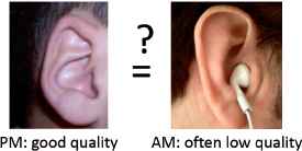
Data quality issues in PM and AM photographs.

Efficiently coping, in a (semi-)automated way, with the different aspects of the comparison of imperfect ear photographs, as taken into account by forensic experts, is a research challenge.

Contribution. Research in medical image processing revealed that working with 3D ear models helps to overcome problems caused by differences in orientation, scaling and resolution of 2D ear pictures. In this paper, we investigate if and how computational intelligence techniques can be used and combined for comparing 3D ear models. More specifically we investigate ear recognition techniques which allow to explicitly reflect forensic expert knowledge on ear identification, and moreover provide semantically richer information on the quality of retrieved results.

The presented work is the further development and integration of two techniques that we separately introduced^5,6. The first technique handles the bipolarity that will arise when distinguishing feature points that are of sufficient (positive pool) or of insufficient quality (negative pool). All the results of comparisons of feature points are expressed using bipolar satisfaction degrees (BSDs)⁷. A BSD quantifies how well two feature points match (or do not match), and additionally assesses the hesitation about that comparison result, which is, e.g., caused by a lower quality of the AM photographs. The second technique is used to split off and compare subsets of feature points that correspond to specific areas of the ear shape. Results of elementary comparisons results are then combined using a hierarchic logic scoring of preferences (LSP)⁸ aggregation structure. This provides us with facilities to adequately model and incorporate (forensic) expert knowledge on ear comparison issues. LSP based comparison as presented in⁵ does not cope with bipolarity at all. Combining both techniques requires that the bipolarity in the data is properly reflected in the aggregation. Handling this is the main novel contribution of this paper.

Structure of the paper. The remainder of the paper is organized as follows. Related work is briefly described and discussed in Section 2. In Section 3, some preliminaries are given. First, some general issues on ear comparison are explained. Second, some basic concepts and definitions of bipolar satisfaction degrees are given. In Section 4, the 3D ear model that is used in our research is introduced. Section 5 deals with ear recognition and comprises the main contribution of the paper. It describes how corresponding (groups of) feature points from two ear models can be compared, using a novel bipolar similarity measure. Furthermore, it describes how this bipolar similarity measure can be used for comparing two 3D ear models. Finally, it explains the interpretation of comparison results in a bipolar setting. The benefits and added value of the novel ear recognition approach are discussed and demonstrated by an illustrative example in Section 6. Finally, some conclusions and plans for further research are reported in Section 7.

2. Related Work

Aspects of ear photograph comparison have been studied in several works^9,10,11,12. An important aspect of an ear comparison process is ear recognition. During ear recognition corresponding features, which are extracted from two ear models, are compared in order to decide whether the associated ears match or not. Most related work on ear recognition is based on machine learning techniques. The considered feature extraction methodology can be used to categorize it.

Intensity based recognition methods use techniques like principal component analysis, independent component analysis and linear discriminant analysis for the comparison^13,14,15. Other categories of recognition methods are based on force field transformations¹⁶, 2D ear curves geometry¹⁷, Fourier descriptors¹⁸, wavelet transformation¹⁹, Gabor filters²⁰ or scale-invariant feature transformation²¹.

A last category of recognition techniques is based on 3D shape features. Most approaches use an iterative closest point algorithm for ear recognition^{22,23,24,25,26,27}. In²⁸ both point-to-point and point-to-surface matching schemes are used, whereas the method in²⁹ is based on the extraction and comparison of a compact biometric signature.

An elaborate survey on ear recognition is contained in³⁰. Another work covering the main aspects of automatic recognition of human ears is³¹.

Only a few recognition approaches^11,12 consider to select specific areas on ear models and compare them in a pairwise fashion. Comparison results are then aggregated to obtain an overall matching score. Weighted aggregation allows assigning a different importance to specific ear parts, which in its turn can be interesting when some parts can be less trusted than others (due to, e.g., data quality issues). Explicitly considering separate ear parts in recognition also supports the reflection of forensic expert knowledge. For example, it is generally known that ears are relatively immune to variation due to ageing⁴. This holds true for the full ear shape, with the exception of the ear lobule which is known to elongate for elderly people. So, when the PM photograph is of a person who is more than seventy years old and the AM photograph is of a person who is much younger, a mismatch of the ear lobule shape should not have a significant impact on the overall ear comparison result. Likewise, some variations of the ear shape are known to be extremely rare. A match for such parts should give a significantly higher indication that the full ear shapes should match too.

To the best of our knowledge, none of the existing ear recognition techniques adequately assess and handle data quality issues. However, assessing data quality and reflecting its impact on the results of ear comparisons is important. Indeed, extra information expressing the quality of the data on which the comparisons are based enriches the comparison results. Forensic experts can use this extra information to improve their decision making. For example, the case where an AM photograph A and a PM photograph P only partially match, while both having sufficient quality, clearly differs from the case where A and P partially match to the same extent, but where A is of (much) lower quality.

3. Preliminaries

4. 3D Ear Model

In previous work, we tried to accomplish ear recognition by using 2D ear images³³. However, imperfect geometric and photometric transformations of 2D AM photos put a limit on the quality of comparison results. To improve upon our previous work we currently work with a 3D ear shape model that captures the three dimensional details of the ear surface, as shown in the left and middle parts of Fig. 2.

Fig. 2.

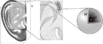
An illustration of our 3D ear model (with hesitation spheres).

5. Ear Recognition

In ear recognition, the feature sets of two right (or two left) ear models are compared. If used for victim identification, the feature set F_P of the PM ear model P of the victim’s right (or left) ear has to be compared with the feature set F_A of the AM ear model A of a missing person’s right (or left) ear.

In this section we propose a novel method for improving the quality of an ear recognition process. In Subsection 5.1, a basic technique for comparing corresponding features of AM and PM feature sets is described. This technique is improved in Subsection 5.2 to explicitly cope with the hesitation that might exist about the data quality. In Subsection 5.3, we study how two 3D ear models and their metadata can be compared. Special attention goes to the adequate modelling of forensic expert knowledge. The interpretation of the results and the added value of our novel approach are discussed in Subsection 5.4.

5.3. Comparing 3D Ear Models

Eq. (10) yields a BSD (s, d), expressing the degree of satisfaction s and the degree of dissatisfaction d about the matching of two corresponding features p^A and p^P. As extra information, the degree of hesitation h = 1 − s − d about the matching can be derived. In order to come to a comparison of two 3D ear models A and P, their feature sets FA={p1A,...,pnA} and FP={p1P,...,pnP} have to be compared. Available metadata (gender, age, race, etc.) about the persons whose ears are being modelled is also taken into account.

The comparison of two feature sets F_A and F_P is done piecewise. Different subsets of the feature sets can be compared separately, after which the resulting BSDs are aggregated using a hierarchical aggregation structure. The BSDs resulting from the evaluation of criteria on the metadata can also be incorporated in the aggregation structure. Moreover, BSDs can be assigned different weights reflecting the relative importance of their associated criteria in the ear recognition process. This approach allows us to reflect and handle forensic knowledge on how to compare ears, in the matching process.

5.3.1. Comparing Corresponding Subsets of Features

The separate treatment of different subsets of feature sets F_A and F_P in the comparison process is motivated by the fact that forensic experts have considerable knowledge about the typicality of specific shapes of different parts of the outer ear. Fig. 3 contains an overview of the most important distinguished ear parts. Also, knowledge about which parts are sensitive to deformations due to ageing, earrings, objects or other phenomenons might be relevant for fine-tuning the ear recognition process.

Fig. 3.

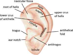
Different parts of an outer ear.

Hence, there is a need for a facility to group all features that belong to an identified part of the ear in a subset and compare corresponding subsets stemming from two 3D ear models. Such comparisons can then later be combined with other comparisons and criteria on the metadata. Feature point selection will in general be guided by the need to distinguish among specific parts of the ear.

Consider a subset FA'={p1'A,...,pk'A}⊆FA and its corresponding subset FP'={p1'P,...,pk'P}⊆FP. Hereby, it is assumed that each feature pi'A∈FA' corresponds to the feature pi'P∈FP', i = 1, . . . , k. The bipolar group similarity between two (corresponding) feature subsets FA' and FP' is defined by the similarity measure fBSimG:

(13)fBSimG:℘k(ℙ)×℘k(ℙ)→[0,1]2   ({p1'A,...,pk'A},{p1'P,...,pk'P})↦(s,d)

where ℘_k(ℙ) denotes the subset of the power set ℘(ℙ) of ℙ that consists of all sets with k elements (1 ⩽ k ⩽ n). With the understanding that (.)_s and (.)_d respectively denote the s and d components of a BSD, the BSD (s, d) in Eq. (13) is defined by:

(14)s=∑i=1k(fBSim(pi'A,pi'P))sk

(15)d=∑i=1k(fBSim(pi'A,pi'P))dk.

So, the (dis)satisfaction degree of the bipolar group similarity between two feature subsets is considered to be the average of the (dis)satisfaction degrees of all corresponding features contained in the subsets. Other definitions are possible here. For example, when a pessimistic approach is used, (s, d) can be defined as being the worst of all the BSDs resulting from the comparisons of the corresponding features, i.e.

(16)(s,d)=arg⁡(min⁡(si,di)∈C(si+(1−di)2))

with C={fBSim(pi'A,pi'P)|i=1,...,k} .

5.3.2. Aggregation Trees for Ear Recognition

At the basis of the comparison of an AM ear model A and a PM ear model P are the comparison(s) of (subsets of) their respective feature sets F_A and F_P — as described above — and the evaluation of meta-data criteria. Metadata criteria can, among others, be used for checking the age, gender or race of two persons, or for checking the presence of characteristics like birthmarks, tattoos and perforations by earrings or piercings.

The result of a metadata criterion evaluation can also be expressed by means of a BSD. Indeed, verifying whether the metadata for A and P match (or not) can yield in a full satisfaction s = 1 (or full dissatisfaction d = 1), which corresponds to the BSD (1, 0) (or (0, 1)). It can also result in a partial (dis)satisfaction caused by some hesitation 0 < h ⩽ 1 which can, e.g., be reflected by the BSD ((1 − h)/2, (1 − h)/2) (cf. Eq. (10)). For example, if A and P are both ear models of a person belonging to the Caucasian race, the comparison criterion for race will yield (1, 0), denoting full satisfaction. However, if there is a hesitation h about the race of P it will result in a partial satisfaction. More details on the specification and evaluation of metadata criteria are not given in this paper.

The next step in the 3D ear model comparison, is the aggregation of the BSDs that are obtained from subset comparisons and metadata criteria evaluations. Aggregation should result in an overall BSD that adequately reflects the similarity between the AM and PM ear models and the hesitation that might exist about this similarity. In order to obtain this, a hierarchic aggregation structure is proposed. An aggregation tree⁸ allows to adequately reflect human decision making and hence can also be configured to model ear comparison strategies that are used by forensic experts⁸.

Aggregation tree structures are constructed as follows. Each leaf node either corresponds to a subset comparison or to a metadata criterion. The evaluation of a leaf node results in a BSD. Each internal node corresponds to an aggregator. Such an aggregator groups (the results of) related subset comparisons and/or metadata criteria. It also supports the modelling of higher abstraction levels that might exist in the decision making. For example, one aggregator can group criteria that check the presence of piercings and earrings. Another aggregator can group criteria that relate to the central parts of the ear (ear notch, tragus, antitragus and antihelix). And yet another aggregator can be used to reflect that similarity of the ear lobules should rather be considered as a bonus (not a requirement) in those cases where the estimated age of the victim is older than seventy and the difference in time of the AM ear photo shoots is significant. We will further develop some of these examples in Section 6.

The evaluation of an internal node involves the aggregation of the BSDs that result from the evaluations of its child nodes and results in a new BSD. This BSD reflects the overall satisfaction and hesitation, considering all subset comparisons and meta-data criteria, which are specified in the subtree that has the internal node as root. Ear model comparison then boils down to (recursively) evaluating the root node of the aggregation tree.

An example of an aggregation tree is depicted in Fig. 4. The solid rectangles at the left side of the figure represent the subset comparisons and metadata criteria. Each comparison and criterion is evaluated, which yields a BSD. These BSDs are the leaf nodes of the tree and form the inputs for the evaluation of the other nodes. Each internal node represents an aggregator and is characterized by a parameter α, which will be introduced next. The inputs of an aggregator have a weight w, as explained below.

Fig. 4.

Example of an aggregation tree.

The aggregators of the aggregation tree are all defined based on the generalized conjunction/disjunction (GCD) function^8,5, which is adapted here to cope with BSDs. Both basic aggregators and partial absorption aggregators are considered.

Basic Aggregators. For each basic aggregator Abα, two kinds of parameters have to be provided: weights and the andness parameter α.

A weight w_i ∈ [0, 1] is assigned with each input (s_i, d_i), 1 ⩽ i ⩽ n of the aggregator. The weights have to sum up to one, i.e., if we have an aggregator with n BSDs as input, ∑i=1nwi=1. In this way, each weight reflects the relative importance of the input to which it is associated.

The andness parameter α ∈ [0, 1] determines the logical behaviour of the aggregator. It acts as an index expressing how ‘close’ the logical behaviour of the aggregator Abα should be to the logical behaviour of the regular conjunction operator. Hence, andness stands for simultaneity, whereas its complement orness (ω = 1 – α) reflects replaceability⁸. The weighted power mean definition of Abα is as following:

(17)Abα:([0,1]2)n×[0,1]n→[0,1]2(((s1,d1),...,(sn,dn)),(w1,...,wn))↦{(min⁡(s1,...,sn),max⁡(d1,...,dn)),  if α=1(max⁡(s1,...,sn),min⁡(d1,...,dn)),  if α=0((∑i=1nwi⋅siq)1/q,∑i=1nwi⋅diq¯)1/q¯),  else

where the exponents q and q¯ (∈] − ∞, +∞[) differ from zero and can be numerically approximated by computing⁸:

(18)(0.25+1.602⋅(0.5−x)+1.051⋅(0.5−x)2+2.163⋅(0.5−x)3−3.390⋅(0.5−x)4)/(α⋅ω)

with x = α for q and x = 1 − α = ω for q¯.

The semantics of the aggregators that are defined by Eq. (17) are completely in line with the semantics of the logical operators that were introduced in Eq. (2)–(4). For α < 0.5 we have disjunction. When α = 0 the disjunction is called full disjunction (D). For 0 < α < 0.25 a hard partial disjunction (HPD) operator is obtained, whereas 0.25 < α < 0.5 yields a soft partial disjunction (SPD) operator. Hence, α = 0.25 can be considered as corresponding to a neutral partial disjunction (PD) operator. Likewise, for α > 0.5 we have conjunction and α = 1 is called full conjunction (C). For 0.75 < α < 1, a hard partial conjunction (HPC) operator is obtained, whereas 0.5 < α < 0.75 yields a soft partial conjunction (SPC) operator. The andness α = 0.75 can be considered as corresponding with a neutral partial conjunction (PC) operator. If α = ω = 0.5, the neutral (weighted) arithmetic mean operator (A) is obtained. In this case q=q¯=1 holds.

Partial Absorption Aggregators. A partial absorption aggregator Aa(α,P,R) is needed for combining a mandatory (or sufficient) input x with an optional input y (cf.^39,40). Partial absorption aggregators have three parameters: the andness α ∈ ]0, 0.25] ∪ [0.75, 1[, a mean penalty percentage P ∈ [0, 100%] and a mean reward percentage R ∈ [0, 100%]. If α ⩾ 0.75, the aggregator is conjunctive, in which case x is interpreted as a mandatory input. If α ⩽ 0.25, the aggregator is disjunctive and x is interpreted as a sufficient input. The penalty and reward percentages are used to adapt the BSD of x in case the optional criterion y is satisfied (resp. not satisfied). In a bipolar setting, a partial absorption aggregator is defined as:

(19)Aa(α,P,R):[0,1]2×[0,1]2→[0,1]2((s1,d1),(s2,d2))↦(s,d)

where

s=((1−w2)⋅(w1⋅s1+(1−w1)⋅s2)q+w2⋅s1q)1/q

and

d=((1−w2)⋅(w1⋅d1+(1−w1)⋅d2)q¯+w2⋅d1q¯)1/q¯.

This definition is an extension of the partial absorption aggregators presented in³⁹, where the neutral aggregator (A) is chosen for the ‘inner’ aggregation and Eq. (18) is used for approximating the exponents q and q¯ of the ‘outer’ aggregation. The weights w₁ and w₂ are computed to reflect, as adequately as possible, the impact of the mean penalty P and mean reward R percentages provided by the user. Hereby, it is considered that the criterion satisfaction is decreased with a penalty of p% if the optional condition is not satisfied at all, and increased with a reward of r% if the optional condition is fully satisfied. The given values P and R are (approximately) the mean values of p and r and are used to compute w₁ and w₂ as described in⁴⁰.

6. Illustrative example

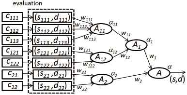
The benefits and enriched expressibility of our proposed approach are discussed and demonstrated by the following illustrative example. Consider the simplified comparison scenario, presented in Fig. 5. An AM ear model A is compared with a PM ear model P. There are two metadata attributes ‘gender’ and ‘race’, whose values, if available, should match. The other six attributes denote subsets of feature points. Attributes ‘antihelix’, ‘tragus’, ‘ear notch’, ‘antitragus’ and ‘lobule’ correspond to specific parts of the ear as depicted in Fig. 3, whereas attribute ‘other parts’ denotes the subset of all other feature points (not included in the subsets of the five previous attributes). The attribute values for A and P are resp. presented in the first and second column next to the attribute name.

Fig. 5.

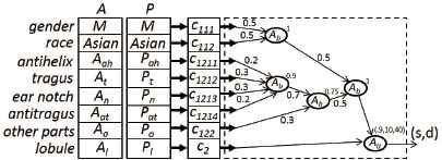
Illustrative example.

For each attribute there is a corresponding elementary criterion. Criteria c₁₁₁ and c₁₁₂ respectively check whether the gender and race of A and P possibly match or not, whereas the other criteria c₁₂₁₁, c₁₂₁₂, c₁₂₁₃, c₁₂₁₄, c₁₂₂ and c₂ compare corresponding subsets of feature points by applying Eq. (13). Each elementary criterion is evaluated with its corresponding attribute values for A and P. The resulting BSDs enter the aggregation structure (dotted box) via their corresponding arrows. (For the sake of clarity, the BSDs are not represented in the figure.)

The aggregation structure reflects (part of) the forensic expert knowledge. The following knowledge rules are reflected:

• •

  Both criteria on the metadata (c₁₁₁ and c₁₁₂) are mandatory and should be fully satisfied in order to conclude a match. This is modelled by a pure conjunctive basic aggregator (α = 1). Weights do not have any impact on this aggregation and are by default set to 0.5.

• •

  Parts of the inner ear are considered to be more important for the matching process. The inner ear parts under consideration are the tragus, ear notch, antitragus and antihelix where the tragus and ear notch are slightly more important than the other two. This is modelled by two basic aggregators. The first aggregator aggregates all results stemming from the comparison of inner ear parts. The results that stem from the tragus (c₁₂₁₂) and ear notch (c₁₂₁₃) comparisons are assigned a slightly higher weight (0.3) than those stemming from the antitragus (c₁₂₁₄) and antihelix (c₁₂₁₁) comparisons (0.2). A hard partial conjunction (α = 0.9) with an andness of 90% is considered. This reflects that all criteria should be satisfied to some extent, but some relaxation of 10% satisfaction is allowed to conclude a match. The second aggregator combines the inner ear comparison result with the result of comparing the other feature points (c₁₂₂), excluding those that belong to the lobule. Respective weights of 0.7 and 0.3 reflect the importance of the inner ear over the other parts. A neutral partial conjunction (α = 0.75) is considered to allow for some relaxation in the matching results.

• •

  The shape of the lobule of elder persons can elongate over time. A solution for coping with this rule is to consider ear lobule matching optional. If the ear lobules (partially) match, a corresponding reward is assigned to the matching score, otherwise a penalty is assigned. This is modelled by a conjunctive partial absorption aggregator (α = 0.9) with mean penalty P = 10% and mean reward R = 40%. Because the partial absorption aggregator is a binary operator, the results of the meta-data comparison and other feature point comparisons first have to be aggregated to obtain a single mandatory input. A pure conjunctive basic aggregator (α = 1) is used. The result of the lobule comparison (c₂) is the optional input.

The above example illustrates the added-value of our proposal. With traditional aggregation techniques the given knowledge rules would be much more difficult to model. Moreover, the aggregation structure takes BSDs as input and generates an over-all BSD (s, d), which also reflects the overall hesitation about the data quality. Such extra information helps the forensic experts to correctly interpret the worth of the comparison results, revealing hints in cases where no adequate matches are found. A more complex aggregation structure is needed for comparing real cases, where more knowledge rules are involved in the comparison process.

A main advantage of the proposed framework is that it offers novel facilities for tackling the challenging problem of comparing a 3D PM ear model obtained from a good 3D image with a 3D AM model obtained from lower quality 2D AM photographs. To the best of our knowledge, this problem has not been studied yet. More research is definitely needed here, but it is already clear that potential solutions would benefit from data quality assessment and configurable representations of forensic expert knowledge.

Current approaches for 3D ear image recognition, as described in Section 2, already yield good comparison results when applied to high quality images. If applied to high quality 3D images (full visibility, no deformations, no difference in age), the recognition approach described above is accurate enough to generate comparable results. Small differences, caused by imperfections in the fitting process, are compensated by the flexibility of the proposed similarity measure (parameters ε₁ and ε₀ in Eq. (9)).

However, adequately dealing with low quality AM photos requires more flexibility for guiding the comparison process in accordance to preferences that are set by forensic experts. Indeed, in these cases, the fitting process will yield larger differences so that untrusted parts should be excluded from the comparison process. (Else, the required compensations would be so large, that a large number of false positives will be inevitable.) The techniques presented in this paper are meant to contribute in offering such a flexibility.

Also, experiments with representative, real-life data sets are required for fine-tuning all the parameters that occur and for validating the approach. Constructing such data sets is time consuming and subject to ongoing work. For example, a representative number of 3D AM ear models containing unreliable parts, representing information from old photos, etc. should be included, as well as ear models of relatives like parents, siblings, twins, etc. In a later stage, 3D ear models obtained from 2D AM photos should also be included.

7. Conclusions and Future Work

The purpose of this paper is proposing a theoretical framework for novel techniques, which make ear comparison more human centric. More specifically, the paper first presents a framework for assessing data quality and reflecting the hesitation caused by bad data quality in the comparison results. This provides decision makers with useful extra information. Another novelty in the paper is the integration of an advanced, configurable aggregation structure, supporting the incorporation of forensic expert knowledge in the comparison process. Configuring the relative weights of the inputs and the andness parameters of the basic aggregators and configuring the penalty, reward and andness parameters of the partial absorption aggregators in the aggregation structure supports decision makers in performing different comparisons for investigating multiple circumstances and scenarios.

The paper focuses on the semantic aspects of the ear comparison problem and demonstrates how computational intelligence techniques help to make ear comparison more human centric. In our future work we plan to focus on the fine-tuning of the similarity measure and the configuration of the aggregation structure. We also plan extensive tests with real-life cases once a database with enough data, obtained from 2D AM photographs, is available. As well the impact on execution time, as the impact on the recognition results of different parameter settings and configurations will be studied.