
A segment-based approach to the analysis of project evaluation problems by hesitant fuzzy sets
- DOI
- 10.1080/18756891.2016.1161344How to use a DOI?
- Keywords
- Hesitant fuzzy set; Group decision making; Project evaluation; Segment-based evaluation
- Abstract
We provide a methodology to perform an extensive and systematized analysis of problems where experts voice their opinions on the attributes of projects through a hesitant fuzzy decision matrix. This provides the decision-maker with ample information on which he or she can rely in order to make the final decision, in the form of segments instead of numbers. These segments derive from weighted average of new parametric expressions for two tenable indices of satisfaction, the distance to an ideal or the similarity to an anti-ideal, and permit to give a profuse unified picture of the relative performance of the projects. When the parameter grows, these indices tend to replicate the evaluation by respective simplistic expressions that only depend on the least, resp., the largest, evaluation and the number of evaluations in each cell.
- Copyright
- © 2016. the authors. Co-published by Atlantis Press and Taylor & Francis
- Open Access
- This is an open access article under the CC BY-NC license (http://creativecommons.org/licences/by-nc/4.0/).
1. Introduction
The classical group decision making problem concerns the context where a group of experts have to make a decision on a set of alternatives, attending to either one or multiple criteria. The experts’ opinions about the alternatives are usually characterized by their knowledge or subjective ideas, which produces a rich environment of models in order to capture the setting and reach a final decision. The literature abounds with references about the decision making process under different positions8,9,13,24,31,36,49,53.
It has long been recognized that fuzzy sets (FS) and fuzzy logic provide useful tools for the management of human subjectivity in decision-making contexts12,21,18,37. However in some practical problems, imprecise human knowledge (and especially group knowledge) cannot be suitably represented by fuzzy sets and some generalizations are needed. This was established as early as in Zadeh50. In this paper we are interested in a new, segment-based methodology that permits to perfom an extensive and systematized analysis of problems that are better modelled by Torra’s38 hesitant fuzzy sets (HFSs, originally considered by Grattan-Guinness16), which incorporate many-valued sets of memberships. The motivation for using this concept in decision making is clearly explained e.g., in Xu46. This reference justifies that hesitant fuzzy elements and sets have produced an extensive theoretical and applied literature 30,32,40,43,56. Furthermore, a recent authoritative survey of HFSs is Rodríguez et al.34. Here the authors summarize many useful and valuable decision making methods to solve hesitant fuzzy multi-criteria decision making problems and propose further applications of HFSs to decision making.
1.1. Our assumptions and research objectives
We focus on the following common situation in multi-criteria decision analysis. We need to compare some alternatives or projects, and some experts evaluate their performance with respect to a set of attributes or characteristics. In this context the group knowledge on each project must be naturally represented by set-valued memberships, instead of just membership degrees as in fuzzy sets. Henceforth not only we permit imprecision or vagueness, but also a touch of uncertainty since we do not attach more value to a voiced opinion than to another one. Then the question arises: How do we analyze the problem of prioritizing these projects?
The formal statement of this question refers to hesitant fuzzy decision matrices (HFDMs), i.e., matrices whose cells contain hesitant fuzzy elements (HFEs). These HFEs collect the opinions voiced by the experts on each attribute of the succesive projects. In our description rows are associated with projects and can be assimilated with HFSs. Thus we want to compare rows in these matrices on the basis of their relative performance (as alternatives or projects).
The problem posed above, i.e., ranking HFSs or HFEs, has received attention from various authors recently. Xia and Xu44 and Farhadinia15 propose to use aggregating operators in order to associate a single HFE with each project. Then score functions give rankings of the aggregate HFEs. Xu and Xia47 rank the projects according to a direct appeal to distances. Finally, Zhou and Li54 design a lexicographic ranking that refines the Xia and Xu proposal44. A summary of these studies related to HFSs/HFEs ranking is given in Table 1.
| Author(s) | Tool(s)/method(s) |
|---|---|
| Xia and Xu44 Farhadinia15 |
Aggregating operators and score functions |
| Xu and Xia47 | Distances and similarities |
| Zhou and Li54 | Lexicographic procedure |
Summary table of studies related to ranking of HFSs or HFEs
In order to make a broader analysis of these decision-making situations we draw inspiration from two sources. In the first place, we observe that the relative inadequacy of the projects (i.e., of their associated HFSs) can be estimated either by the ‘distance’ to an ideal HFS or the ‘similarity’ to an anti-ideal HFS, in the sense that the higher these evaluations the worse the project’s performance. Here we suggest respective novel parametric indicators for such proxies that incorporate the relative importance of the attributes through ex-ante allocations of weights. Their asymptotic behavior, i.e., the role of the parameter, is disclosed: when the parameter goes to infinity these indicators tend to provide an evaluation by respective simplistic expressions that only depend on the least, resp., the largest, evaluation and the number of evaluations on each attribute. In the second place, we draw inspiration from the Hurwicz approach to decision making under uncertainty26, which advocates for the combined use of ‘best and worst outcomes’ to assess the value of uncertain decisions. Thus the Hurwicz approach permits us to combine our two plausible parametric indices by their weighted sums, which includes both indices as extreme cases5. Their limit behavior replicates the case of the original indicators. Now for each project we obtain a segment instead of a single number, which can provide a richer analysis of the decision problem. Obviously, for any choice of the averaging aggregator a concrete ranking of projects arises.
We also report on the results of an experimental example that illustrates our proposal. In particular, we carry out a sensitivity analysis that permits to visualize the limit behaviour of our indexes in the analysis of problems characterized by HFDMs (e.g., hierarchization of projects characterized by HFSs). Finally, our approach is compared with other evaluation methods proposed by Xu46.
1.2. Literature review: Project evaluation problems
Multi-criteria decision making methods (MCDM) focus on the implementation of Decision Theory in real-life problems. One of the the most complex real situations is the evaluation of projects because it includes various factors and criteria. There exist different MCDM techniques to provide solutions to this problem. The appropriateness of the method depends on the specific decision situation39. Some examples of such decision contexts are: new product development projects10, energy projects19, information technology projects3, investment projects2, etc.
Other contributions include some simple examples of different MCDM methodologies about project evaluation20,23,35. When the projects can begin on different time moments, the research on this problem is limited6,25,29.
From another point of view, Fuzzy Set Theory has been extensively used to model uncertainty and vagueness associated with project information sources. And it has been gradually gaining importance as a tool in project selection4,7,17,27. Two milestones in this regard are Wang and Hwang41 (who develop a fuzzy integer programming model to gain an optimal investment portfolio), Chiu et al.11 and Wang et al.42 (who apply the fuzzy concept to the project selection process with the fuzzy multi-criteria decision-making model (FMCDM) to select the optimal alternative).
Within the extended field of Hesitant Fuzzy Sets, which allows for cases with several degrees of membership, there are many application papers that contribute to Multicriteria Decision Making Theory 1,22,44,48,52,51,54. Multiexpert multicriteria decision making under this requirement has been explored by Xia et al.45.
A summary of these studies related to the evaluation problem is given in Table A.5.
1.3. Organization of the paper
The remaining of this paper is organized as follows. Section 2 establishes some basic definitions. Section 3 introduces our proposals for ranking hesitant fuzzy sets, as well as results concerning the asymptotic behavior of our indices. In Section 4 we put in practice the methodology that permits to study the hierarchization of projects characterized by hesitant fuzzy sets. We visualize the asymptotic behavior of our indexes in a fully developed example, and then our results are confronted with the evaluations in existing approaches. We conclude in Section 5.
2. Notation and definitions
For any (possibly infinite) set A, 𝒫*(A) denotes the set of non-empty subsets of A, and ℱ*(A) denotes the set of non-empty finite subsets of A.
Definition 1. 44
A hesitant fuzzy element (HFE) is a non-empty, finite subset of [0, 1]. The set of HFEs is denoted by ℱ *([0, 1]).
Henceforth we refer to X, a fixed set of alternatives.
Definition 2. 38
A hesitant fuzzy set (HFS) on X is a function from X to 𝒫*([0, 1]).A typical hesitant fuzzy set on X is a function from X to ℱ*([0, 1]). HFS(X) means the set of HFSs on X, and the set of typical HFSs on X is denoted by HFS(X).
Unless otherwise stated, HFSs are assumed to be typical.
Formally speaking, a (typical) HFS is a subset M ⊆ X × ℱ*([0, 1]) such that for each x ∈ X, there is exactly one element hM(x) ∈ ℱ*([0, 1]) such that (x, hM(x)) ∈ M.
Each HFS on X defines a set of membership values for each element of X, and in the case that the HFS is typical such set is always finite. HFEs represent the set of possible membership values of a typical hesitant fuzzy set at an alternative.
By restricting ourselves to either ℱ*([0, 1]) or 𝒫*([0, 1]), i.e., non-empty HFEs, we disregard ‘nonsense elements’ in each HFS: on each alternative, at least one assessment must be made.
From a practical point of view, Xia and Xu44 show that the hesitant fuzzy set M can be represented as M = {(x, hM(x)) | x ∈ X}. For example, following Torra38 we define
Clearly, when all HFEs involved in the definition of an HFS on X are singletons we can identify such HFS with a fuzzy set (FS) on X. That is to say, HFEs of the form
Now we proceed to formalize the general concepts of distance and similarity between HFSs.
Definition 3. [Xu and Xia 47]
A distance measure between HFSs on X is a function d : HFS(X) × HFS(X) → [0, 1] that satisfies the following properties: for every M, N ∈ HFS(X),
- 1.
0 ⩽ d(M, N) ⩽ 1;
- 2.
d(M, N) = 0 if and only if M = N;
- 3.
d(M, N) = d(N, M).
Definition 4. 47
A similarity measure between HFSs on X is a function s : HFS(X) × HFS(X) → [0, 1] that satisfies the following properties: for every M, N ∈ HFS(X),
- 1.
0 ⩽ s(M, N) ⩽ 1;
- 2.
s(M, N) = 1 if and only if M = N;
- 3.
s(M, N) = s(N, M).
There are similitudes between the latter concepts. When d is a distance measure between HFSs on X, the expression s = 1 − d defines a similarity measure between HFSs on X. Conversely, when s is a similarity measure between HFSs on X, the expression d = 1 − s defines a distance measure between HFSs on X. Besides Xu and Xia47, Xu46 collects many other examples of distance functions between HFSs in the literature.
3. Ranking typical HFSs: the segment approach
In this Section we consider the analysis of the following problem. There are m alternatives or projects whose performance with regard to n criteria or attributes is evaluated by a team of experts (in a range from 0 to 1). Each expert can be hesitant on the performance of the projects, therefore he or she can emit any finite number of evaluations to express his or her doubts. For each project, all evaluations by the experts on each criteria are collected into a set of values. This presumes anonymity of the experts: all opinions are equally considered in this process. Formally, this produces an HFS associated with the project: for each attribute, a finite set of values in [0,1] is given. We face a problem under complete uncertainty: the importance of each particular appraisal is totally unknown.
The opinions of the experts can be captured by a hesitant fuzzy decision matrix (HFDM), i.e., an m × n matrix whose cells contain HFEs, in such way that its rows trivially define HFSs (one for each project). Columns correspond to respective evaluations of the projects by fixed criteria.
Suppose that we need to rank or prioritize the projects. The problem arises: How do we analyze the decision problem posed?
3.1. Analysis of the problem: the segment approach
Several contributions have dealt with the problem posed above. Xia and Xu44 start by using aggregating operators in order to associate an HFE with each project, and then use a score function to rank them. Farhadinia15 proposes a variation with a different score function. Xu and Xia47 proceed in a more direct way: they rank the projects according to their distance to the ideal HFS. Finally, Zhou and Li54 do not produce evaluations of projects but give a lexicographic ranking that refines the proposal44.
Our proposal intends to make a richer analysis by segments instead of points: with each project we associate a segment rather than a position or a number. It has two sources of inspiration.
Firstly, we draw inspiration from the approach in Xu and Xia47. In order to analyze the relative performance of the projects (or of the HFSs that characterize them) we build on two relevant indicators, namely the ‘distance’ to the ideal HFS and the ‘similarity’ to the anti-ideal HFS. Both seem tenable indices of fitness for an HFS although of course, many distance and similarity indices can be used in analogy with the many proposals of distances between HFSs in the literature. In order to avoid confusions here we develop the model with a single concrete specification, namely, Definition 5 below that slightly echoes the use of the generalized hesitant weighted distance47. We leave the details of possible variations to the interested reader, i.e., specifications that replace our indicators in Definition 5 by expressions inspired on (i) the generalized hesitant weighted Hausdorff distance or the generalized hybrid hesitant weighted distance47 –among other distances between HFSs– or (ii) the ideas of the closedly related paper Xu and Xia48.
We assume that each of the attributes has associated a weight wi such that w1 + ... + wn = 1. Weights are indicative of the relative importance of the attributes, hence a zero weight would mean a dispensable criteria that can be omitted in the analysis. This means that we do not lose generality if we assume wi > 0 for each i henceforth.
Definition 5.
Given λ > 0 and w = (w1,...,wn) with wi > 0 for each i and w1 + ... + wn = 1, the λ-adjusted hesitant weighted distance to the ideal HFS is defined as
Observe
Lemma 1.
If λ = 1 and w =(w1,...,wn) verifies wi > 0 for each i and w1 + ... + wn = 1, then
Proof.
For every M ∈ HFS(M),
The higher the evaluation of an HFS by
Remark 1.
As a consequence of Lemma 1, when λ = 1 a unique ranking is obtained independently of the value of the parameter α because when w = (w1,...,wn) verifies wi > 0 for each i and w1 + ... + wn = 1, then
Figure 1 graphically displays the structure and the flexibility of our approach. Besides the aforementioned intuition for the α parameter, subsection 3.2 below intends to help us understand the role of the λ parameter.
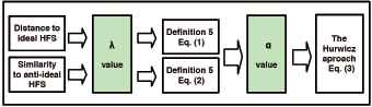
The segment approach to the analysis of project evaluation problems. The use of the α and λ parameters gives flexibility to our approach.
3.2. Asymptotic behavior of the indicators: interpretations
We proceed to check that using our indicators with ‘large’ values of the λ parameter produces evaluations that are increasingly similar to those that derive from very simple indicators. Such indicators are crude evaluations that only rely on the number of different evaluations for each attribute and either the maximum or the minimum of such respective values. To this purpose let us define
Proposition 2.
For every M ∈ HFS(X),
Proof.
We appeal to some basic properties of the lp norms on any ℝt, defined as
We first observe that when M ∈ HFS(M),
An intuitive interpretation is in order.
4. Experimental study
In this section we give an experimental example to illustrate our proposal for the analysis of the hierarchization of projects respectively defined by hesitant fuzzy sets (HFSs). We also carry out a sensitivity analysis of the final outcomes in order to demonstrate the adaptability of the proposed model. Finally, we compare our conclusions with the evaluation methods proposed by Xu46, which provides experimental arguments supporting our approach.
4.1. Evaluation framework
Our example builds on the discussion in Xu and Xia47 which is adapted from Kahraman and Kaya19. Accordingly, let us suppose a society which has to compare five energy projects, denoted by alternatives Ai (i = 1,..., 5). Four energy experts evaluate the performance of the five alternatives with respect to four main attributes or criteria (the example only collects all of the different possible values for each alternative and each attribute)‡:
- •
P1: Technological. In this criterion aspects like technical feasibility, technical risk, access to technology by local agents, maturity of projects, readiness of the local agents to implement the project, multiplicative effects on the local technology basis are taken into account.
- •
P2: Environmental. Based on the project environmental impact.
- •
P3: Socio-political. Included features like the consistency of the project with the society energy policy objectives, the political acceptance of the project, the social acceptance of the project, the scope of the project vs needs to be satisfied-urgency, the appropriateness of the implementing organization, etc.
- •
P4: Economic. Estimated full cost of the project.
The criteria significance fixed by the society is 15% for technological, 30% for environmental, 20% for socio-political and 35% for economic. Consequently the attribute weight vector used along the example is w = (0.15, 0.3, 0.2, 0.35).
The evaluations of the experts on the energy projects, which are based on the aforementioned criteria, are contained in a HFDM (see Figure 2 and Table 2).
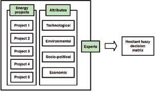
Experimental study evaluation framework
| P1 | P2 | |
|
|
||
| A1 | {0.5,0.4,0.3} | {0.9,0.8,0.7,0.1} |
| A2 | {0.5,0.3} | {0.9,0.7,0.6,0.5,0.2} |
| A3 | {0.7,0.6} | {0.9,0.6} |
| A4 | {0.8,0.7,0.4,0.3} | {0.7,0.4,0.2} |
| A5 | {0.9,0.7,0.6,0.3,0.1} | {0.8,0.7,0.6,0.4} |
|
|
||
| P3 | P4 | |
|
|
||
| A1 | {0.5,0.4,0.2} | {0.9,0.6,0.5,0.3} |
| A2 | {0.8,0.6,0.5,0.1} | {0.7,0.4,0.3} |
| A3 | {0.7,0.5,0.3} | {0.6,0.4} |
| A4 | {0.8,0.1} | {0.9,0.8,0.6} |
| A5 | {0.9,0.8,0.7} | {0.9,0.7,0.6,0.3} |
Hesitant fuzzy decision matrix
4.2. Analysis of the hierarchization of projects: The segment approach
In order to analyze the relative performance of the projects by means of the segment approach, we first need to produce the ‘distance’ to the ideal HFS and the ‘similarity’ to the anti-ideal HFS of each project, as measured by concrete realizations of λ in Definition 5. To be precise, we specify the outcomes when λ = 1, λ = 2 and λ = 20. Finally, we illustrate the asymptotic behavior of the indicators when λ is large enough by comparing these outcomes with the much simpler indicators in subsection 3.2.
- •
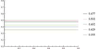
Case λ = 1. Table 3 shows the results of the computations for
- •
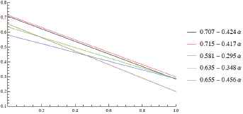
Cases λ = 2, λ = 20. Tables 4 and 5 show the results of the respective computations for these values.
In order to compare the projects under a given choice of λ, the corresponding five segments
- •
Case λ → ∞. Table 6 shows the results of the computations for A and B and also the respective values of Iα as a function of α ∈ [0,1].
A graphical display of the indicators
A graphical display of the indicator
A graphical display of the indicator
| Alternatives | |
|---|---|
| A1 | 0.477 |
| A2 | 0.502 |
| A3 | 0.402 |
| A4 | 0.429 |
| A5 | 0.355 |
Elements for the analysis when λ = 1
| Index | A1 | A2 |
|
|
||
| 0.283 | 0.298 | |
| 0.707 | 0.715 | |
| 0.707 − α0.424 | 0.715 − α0.417 | |
| Index | A3 | A4 |
| 0.286 | 0.287 | |
| 0.581 | 0.635 | |
| 0.581 − 0.295α | 0.635 − 0.348α | |
| Index | A5 | |
| 0.198 | ||
| 0.655 | ||
| 0.655 − 0.456α | ||
Elements for the analysis when λ = 2
| Index | A1 | A2 |
|
|
||
| 0.217 | 0.227 | |
| 0.795 | 0.786 | |
| 0.795 − 0.577α | 0.786 − 0.559α | |
| Index | A3 | A4 |
| 0.241 | 0.242 | |
| 0.660 | 0.714 | |
| 0.660 − 0.419α | 0.714 − 0.471α | |
| Index | A5 | |
| 0.153 | ||
| 0.773 | ||
| 0.773 − 0.620α | ||
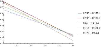
Elements for the analysis when λ = 20
| Index | A1 | A2 |
|
|
||
| A | 0.217 | 0.227 |
| B | 0.795 | 0.786 |
| Iα | 0.795 − 0.578α | 0.786 − 0.559α |
| Index | A3 | A4 |
| A | 0.241 | 0.242 |
| B | 0.660 | 0.715 |
| Iα | 0.660 − 0.419α | 0.715 − 0.472α |
| Index | A5 | |
| A | 0.15325 | |
| B | 0.77425 | |
| Iα | 0.77425 − α0.621 | |
Limit values of the indicators. Iα denotes αA + (1 − α)B.
These segments –one for each project– are uniquely determined by the HFDM. In Figure 6, the Iα (Ai) segments are plotted. We recall that they only depend on the least and the largest evaluation and the number of evaluations in each cell.
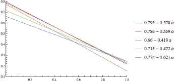
A graphical display of the indicator Iα = α A + (1 − α)B.
With respect to the asymptotic behavior it can be checked that the evaluations of the projects by the
A possible criticism to this approach is that it is fairly complex and certain factors (the λ and α parameters) must be fixed. This seems to introduce ambiguity in the process of decision-making. Nevertheless we must point out that (i) this apparent inconvenience is common to many approaches in exactly the same setting, as subsection 4.3 below recaps; and (ii) the usual role of the analyst is to provide the decision-maker with as much information as possible, rather than making decisions. In this regard, note that our analysis provides visual information in the form of a two-dimensional graph for each choice of λ. The asymptotic behavior of these graphs (or the corresponding indexes) reveals that with only a few properly selected graphs, a complete assessment can be made.
4.3. Discussion of the experimental study
With the results of our experimental example set out, we now proceed to compare them with the rankings obtained from different methodologies that rank HFSs.
We begin with the procedure in Xu and Xia47. Table A.1 contains rankings proposed by the generalized hesitant weighted distance (dghw), the generalized hesitant weighted Hausdorff distance (dghnh), the generalized hybrid hesitant weighted distance (dghhw) and the generalized hesitant ordered weighted distance (dghow). The authors give rankings for several choices of the λ parameter that we adopt for comparison.
In Xia and Xu44, Section 4, the authors proposed to use a GHFWAλ operator (generalized hesitant fuzzy weighted averaging operator, which requires to fix a weight vector and depends on a λ factor) in order to aggregate HFEs, and then rank the resulting HFEs according to their 𝒮1 score
Rodríguez et al.34, Section 4, reported on many other alternative aggregators on HFEs, like GHFWGλ, GHFOWA or GHFOWG44 or QHFOWA, HFMOWA and HFMOWG45. Furthermore, Farhadinia’s 𝒮2 score or any other score on HFEs can be employed as an altermative to 𝒮1. Recall that Farhadinia15 proposed to start with a monotone non-decreasing sequence {δ(1),...,δ(n),...} of positive numbers and then use the score
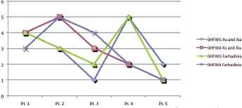
In Table A.2 we have computed the prioritizations with the GHFWGλ and GHFWAλ aggregators, coupled with Xia and Xu’s score. In Table A.3 we have computed the prioritizations with the same aggregators, coupled with Farhadinia’s score.
In contrast, and for the current values of λ, Table A.4 shows rankings backed up by our methodology for five values of the α parameter.
It seems difficult to reach clear-cut conclusions from any comparison, since already the previous analyses in Tables A.1, A.2 and A.3 show disparities among the rankings of the projects without a precise knowledge of their expected behavior. To check these differences Figures 7 to 10 (which illustrate the conclusions of Table A.1) and then Figures 11 to 14 (which illustrate the conclusions of Tables A.2 and A.3) are helpful and indicative. However by comparing Tables A.1 and A.4 we can note the following fact that supports the use of our segment approach with an α parameter. Averaging the
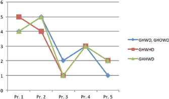
A graphical display of the ranking of the five projects: application of four distances with λ = 1.
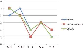
A graphical display of the ranking of the five projects: application of four distances with λ = 2.
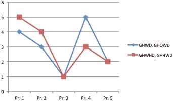
A graphical display of the ranking of the five projects: application of four distances with λ = 6.

A graphical display of the ranking of the five projects: application of four distances with λ = 10.
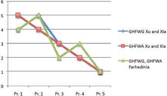
A graphical display of the ranking of the five projects: application of aggregation operators with λ = 1 followed by 𝒮1 and 𝒮2 scores.
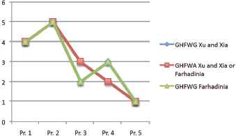
A graphical display of the ranking of the five projects: application of aggregation operators with λ = 2 followed by 𝒮1 and 𝒮2 scores.
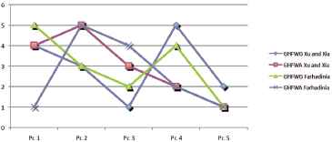
A graphical display of the ranking of the five projects: application of aggregation operators with λ = 6 followed by 𝒮1 and 𝒮2 scores.
A graphical display of the ranking of the five projects: application of aggregation operators with λ = 10 followed by 𝒮1 and 𝒮2 scores.
Let us also stress that our graphical illustrations prove that using both the
5. Conclusion
We have provided a novel methodology that permits to perform an extensive and systematized analysis of problems with a precise specification: experts voice their opinions on the attributes of projects through a hesitant fuzzy decision matrix, that is, an m × n matrix whose cells contain HFEs. Under a specific parametric expression for two reasonable indices of satisfaction, a weighted average permits to give a profuse picture of the relative performance of the projects. A distinctive novel feature of our indicators is that the role of the parameter has been disclosed: when it grows the two indices tend to replicate the evaluation by respective simplistic expressions that only depend on the least, resp., the largest, evaluation and the number of evaluations in each cell. All these elements permit the analyst to provide the decision-maker with ample information on which he or she can rely in order to make the final decision. Moreover, an extensive graphical and numerical analysis of an example from Kahraman and Kaya 19 is confronted with the corresponding analysis in Xu and Xia 47.
With respect to related future lines of research, we already mentioned that replacing our indicators with other potentially useful expressions gives direct variations of our proposal. Particularly, the ideas in Xu and Xia 48 could be adapted to this purpose. Furthermore, the analysis of the analog problem under hesitant fuzzy linguistic information comes to mind as another natural possibility (cf., e.g., hesitant fuzzy linguistic term sets introduced by Rodríguez, Martínez and Herrera 33, see also Zhu and Xu 55).
Acknowledgement
The authors thank the Editors of the International Journal of Computational Intelligence Systems, two anonymous referees, Francisco Herrera and Luis Martínez for their valuable comments and suggestions. Financial support by the Spanish Ministerio de Ciencia e Innovación under Projects ECO2012–31933 and ECO2015–66797–P (J. C. R. Alcantud), ECO2012–32178, CGL2008–06003–C03–03/CLI and ECO2015–66797–P (R. de Andrés Calle), is gratefully acknowledged.
Appendix A
| λ | dghw | dghwh |
|---|---|---|
| 1 | A5 ≻ A3 ≻ A4 ≻ A1 ≻ A2 | A3 ≻ A5 ≻ A4 ≻ A2 ≻ A1 |
| 2 | A5 ≻ A3 ≻ A4 ≻ A1 ≻ A2 | A3 ≻ A5 ≻ A4 ≻ A2 ≻ A1 |
| 6 | A3 ≻ A5 ≻ A2 ≻ A1 ≻ A4 | A3 ≻ A5 ≻ A4 ≻ A2 ≻ A1 |
| 10 | A3 ≻ A5 ≻ A2 ≻ A1 ≻ A4 | A3 ≻ A5 ≻ A4 ≻ A2 ≻ A1 |
| λ | dghhw | dghow |
|---|---|---|
| 1 | A3 ≻ A5 ≻ A4 ≻ A1 ≻ A2 | A5 ≻ A3 ≻ A4 ≻ A1 ≻ A2 |
| 2 | A3 ≻ A5 ≻ A4 ≻ A2 ≻ A1 | A5 ≻ A3 ≻ A4 ≻ A2 ≻ A1 |
| 6 | A3 ≻ A5 ≻ A4 ≻ A2 ≻ A1 | A3 ≻ A5 ≻ A2 ≻ A1 ≻ A4 |
| 10 | A3 ≻ A5 ≻ A2 ≻ A4 ≻ A1 | A3 ≻ A5 ≻ A2 ≻ A1 ≻ A4 |
Rankings obtained by the Xu and Xia’s distances47
| λ | GFWGλ | GFWAλ |
|---|---|---|
| 1 | A5 ≻ A3 ≻ A4 ≻ A1 ≻ A2 | A5 ≻ A4 ≻ A3 ≻ A1 ≻ A2 |
| 2 | A5 ≻ A3 ≻ A4 ≻ A1 ≻ A2 | A5 ≻ A4 ≻A3 ≻ A1 ≻ A2 |
| 6 | A3 ≻ A5 ≻ A2 ≻ A1 ≻ A4 | A5 ≻ A4 ≻ A3 ≻ A1 ≻ A2 |
| 10 | A3 ≻ A5 ≻ A2 ≻ A1 ≻ A4 | A5 ≻ A4 ≻ A3 ≻ A1 ≻ A2 |
Rankings obtained by different HFSs aggregation operators and Xu and Xia score 44
| λ | GFWGλ | GFWAλ |
|---|---|---|
| 1 | A5 ≻ A3 ≻ A4 ≻ A1 ≻ A2 | A5 ≻ A4 ≻ A3 ≻ A1 ≻ A2 |
| 2 | A5 ≻ A3 ≻ A4 ≻ A1 ≻ A2 | A5 ≻ A4 ≻ A3 ≻ A1 ≻ A2 |
| 6 | A5 ≻ A3 ≻ A2 ≻ A4 ≻ A1 | A5 ≻ A4 ≻ A1 ≻ A3 ≻ A2 |
| 10 | A5 ≻ A3 ≻ A2 ≻ A1 ≻ A4 | A5 ≻ A4 ≻ A1 ≻ A3 ≻ A2 |
Rankings obtained by different HFSs aggregation operators and Farhadinia score 15
| λ | α | |
|---|---|---|
| 1 | - | A5 ≻ A3 ≻ A4 ≻ A1 ≻ A2 |
|
|
||
| 2 | α = 0 | A3 ≻ A4 ≻ A5 ≻ A1 ≻ A2 |
| α = 0.25 | A3 ≻ A5 ≻ A4 ≻ A1 ≻ A2 | |
| α = 0.5 | A5 ≻ A3 ≻ A4 ≻ A1 ≻ A2 | |
| α = 0.75 | A5 ≻ A3 ≻ A4 ≻ A1 ≻ A2 | |
| α = 1 | A5 ≻ A1 ≻ A3 ≻ A4 ≻ A2 | |
|
|
||
| 6 | α = 0 | A3 ≻ A4 ≻ A5 ≻ A2 ≻ A1 |
| α = 0.25 | A3 ≻ A4 ≻ A5 ≻ A1 ≻ A2 | |
| α = 0.5 | A3 ≻ A5 ≻ A4 ≻ A1 ≻ A2 | |
| α = 0.75 | A5 ≻ A3 ≻ A4 ≻ A1 ≻ A2 | |
| α = 1 | A5 ≻ A1 ≻ A2 ≻ A3 ≻ A4 | |
|
|
||
| 10 | α = 0 | A3 ≻ A4 ≻ A5 ≻ A2 ≻ A1 |
| α = 0.25 | A3 ≻ A4 ≻ A5 ≻ A2 ≻ A1 | |
| α = 0.5 | A3 ≻ A5 ≻ A4 ≻ A1 ≻ A2 | |
| α = 0.75 | A5 ≻ A4 ≻ A3 ≻ A1 ≻ A2 | |
| α = 1 | A5 ≻ A1 ≻ A4 ≻ A2 ≻ A3 | |
Rankings obtained by the segment approach
| Author(s) | Tool(s)/method(s) |
|---|---|
| Multi criteria decision making-based studies | |
|
|
|
| Carazo et al.6, Lawson et al.20, | POMETHEE, TOPSIS, Data envelop analysis (DEA), |
| Liberatore23, Liu and Wang25, | Analytic hierarchy process (AHP), |
| Medaglia et al.29, Santhanam and Kyparisis35 | Analytic network process (ANP) |
|
|
|
| Fuzzy logic-based studies | |
|
|
|
| Buyukozkan and Feyzioglu 4, Chen et al.7, | Fuzzy POMETHEE, Fuzzy TOPSIS, |
| Chiu et al.11, Huang et al.17, | |
| Machacha and Bhattacharya27, Wang and Hwang41 | Fuzzy DEA, Fuzzy AHP, Fuzzy ANP |
|
|
|
| Alcantud, de Andrés Calle and Torrecillas1, | |
| Farhadinia15, Liao and Xu22, Xia and Xu44, | Hesitant fuzzy logic-based studies |
| Xu and Xia48, Zhang and Xu51,52, Zhou and Li54 | |
Summary table of studies related to evaluation projects
Footnotes
Distance and similarity measures under hesitant fuzzy environment and their properties were put forward in Xia and Xu47
When 0 < p < 1 such expression does not define a norm, although
Figure 6 (see Table 6 instead) shows that the same is true when λ = 20. In this case project A5 is strictly better than A3 which is better than the other projects, under the choice α = 0.5. This coincides with Xu and Xia’s recommendation. However A1 is better than A3 when α = 1, and A4 is better than A5 when α = 0.
References
Cite this article
TY  - JOUR
AU  - José Carlos R. Alcantud
AU  - Rocío de Andrés Calle
PY  - 2016
DA  - 2016/04/01
TI  - A segment-based approach to the analysis of project evaluation problems by hesitant fuzzy sets
JO  - International Journal of Computational Intelligence Systems
SP  - 325
EP  - 339
VL  - 9
IS  - 2
SN  - 1875-6883
UR  - https://doi.org/10.1080/18756891.2016.1161344
DO  - 10.1080/18756891.2016.1161344
ID  - Alcantud2016
ER  -