
A New Default Intensity Model with Fuzziness and Hesitation
- DOI
- 10.1080/18756891.2016.1161345How to use a DOI?
- Keywords
- Intensity model; Fuzziness and Hesitation; Triangular intuitionistic fuzzy numbers; CDS pricing
- Abstract
With the increased financial market volatility, corporate defaults will suffer from the double impact of the external shocks and internal contagion effects. In the existing stochastic default intensity models, the valuation of sensitivity parameters requires a lot of historical data, however, the limited market data does not guarantee the accuracy of parameter estimation, meanwhile, due to the people have a lot of fuzziness and hesitation judgements on the default process, it is necessary for us to let the corresponding random parameter of the default intensity to be a triangular intuitionistic fuzzy interval value. In this paper, we propose a new default intensity model based on the external shocks and internal contagion effects, and introduce the triangular intuitionistic fuzzy numbers into the credit default swaps (CDS) pricing modeling to describe the fuzziness and hesitation of the default process. In the end, we get a new fuzzy form pricing formula for CDS, and by the simulation analysis, we obtain that, all kinds of fuzziness and hesitation of the market have significant impact on credit spreads, and a model result with a consideration of the fair price of CDS in a fuzzy random environment including a pure random environment result. Compared with the existing stochastic model, these proper interval results can offer the investors more flexible options and can more reflect the impact of market environment on credit spreads.
- Copyright
- © 2016. the authors. Co-published by Atlantis Press and Taylor & Francis
- Open Access
- This is an open access article under the CC BY-NC license (http://creativecommons.org/licences/by-nc/4.0/).
1. Introduction
In the U.S. subprime crisis, the collapse of major financial institutions such as Bell Sten and Lehman, aroused people’s common concern, because a large number of counterparty suffered huge losses, lead to the counterparty credit default management has become a hot spot in the theory. As Lando1 pointed out, the default intensity of company is a function of the market state variables, including stock prices, market credit rating, and other variables that cause company defaults, that is, the external shocks are the important sources of default events. When the company have a default event due to the external market shocks, then there may exist counterparty risk between different companies, that is, the default of a company may lead the other one to the economic crisis or even default scenario, which the infected company has a direct economic relationship with the default one. The counterparty risk model reflects the counterparty’s default correlation, it can explain the default aggregation phenomenon in the financial market, and can also reflect the internal dependencies on the default intensity of companies. Jarrow and Yu 2 inspired by the financial crisis events happened frequently in recent years, directly introduced the default contagion effect into the default intensity of survival companies, that is, when a company is in default, the default intensity of other survival companies will have an upward jump, this is the intuitive parameterization of counterparty risk, the related researches can also be see in literatures 3,4. Further more, Bai et al 5 pointed out, the effect of one company’s default on the other company’s default intensity will weaken gradually over time, until zero. That means after a period of time, the default intensity of the other company will rely only on the company itself and the external economic factors, while the impact of the default company’s credit contagion will be minimal, they called this phenomenon an attenuation effect of default contagion.
Meanwhile, with a general view of the literatures available about credit risk analysis and derivatives pricing, the common characteristic of them can be summarized as that almost all the pricing processes are built on the base of the theory of random probability 6–10. Li and Han 11 pointed out, the existed credit risk analysis and derivatives pricing models payed more attention to the strict technical constraints on the mathematical expression, and more attention to the price of risk a future point in time, the basic premise of above discussion is the economic behavior of people can make an exact estimation for the uncertain states of nature, including the Black-Scholes pricing model, Stochastic Interest Rate model and Stochastic Volatility model and so on, assumed that there is only one probability measure, and used random theory to depict the uncertainty of pricing problems. However, due to the characteristics of over-the-counter (OTC) exchange (such as non-standardization of products, the short of strict management system and so on), which will lead to the lack of transparency in transactions, and cause the investors produce a certain fuzziness and hesitation on the counterparty credit default, make the basic premise subject to significant challenges. So that, the existed literatures present some inherent problems, such as the model parameters can not be determined accurately, the empirical data is not obvious and so on. Deep talk, they ignored the complexity of the mutual influence between the pricing model and the real market environments, ignored the fuzzy uncertainty of the mutual influence between the credit risk contagion and the risk measure, thus from one perspective, they given up the basic uncertainty description. Therefore, using fuzzy analysis to study such problems as default probability or derivatives pricing has practical needs.
There have existed some literatures about option pricing in fuzzy random environments, such as, Yoshida 12 introduced the fuzzy logic to the stochastic financial model, and derived a new model on European options with uncertainty of both randomness and fuzziness, Wu 13 pointed out that owing to the fluctuation of financial market from time to time, the volatility and stock price may occur imprecisely in the real world, therefore, he employed the extension principle in fuzzy sets theory to the Black-Scholes formula, and derived a new model on European options, and turned the European call and put option price into a fuzzy number, Xu et al 14 pointed out that the rate λ of Poisson process and jump sequence in the Merton’s normal jump-diffusion model cannot be expected in a precise sense, so they presented a fuzzy normal jump-diffusion model for European option pricing, with uncertainty of both randomness and fuzziness in the jumps, and obtained the crisp weighted possibilistic mean normal jump-diffusion model, the related researches can also be see in literatures 15–18. However, as far as we know, there are few about credit risk analysis and derivatives pricing model under fuzzy environments. E.Agliardi and R.Agliardi 19–20 first proposed a structural model for defaultable bonds in a fuzzy environment, they assumed the assets value is a fuzzy stochastic process, the assumption is related to the investors’ subjective belief about the reliability of the accounting data of the firm, and the duration analysis show that the fuzziness of the stochastic underlying assets have material impact on the term structure of credit spreads. Vassiliou 21 proved that a fuzzy market is viable if and only if an equivalent martingale measure exists, and constructed the forward probability measure, described the evolution of credit migration of a defaultable bond as an inhomogeneous semi-Markov process with fuzzy states, and investigated the asymptotic behaviour of the survival probability in each fuzzy state given in the absence of default. Wu and Zhuang 22 proposed a reduced-form intensity-based model under fuzzy environments, and presented some applications of the methodology for pricing defaultable bonds and credit default swaps, but they ignored the important effect of counterparty risk and attenuation effect on the default company. For those existed models, their advantages and disadvantages can be summarized as the following Tab 1.
| The author | The main conclusion | Advantages | Disadvantages |
|---|---|---|---|
| Agliardi, E and Agliardi, R 19– 20 |
Proposed a structural model for defaultable bonds in a fuzzy environment. | Through the imperfect information collection can relax the default predictability of structural model. | No simulation calculate to verify this model. |
| Vassiliou P C G 21 | Described the evolution of credit migration of a defaultable bond as an inhomogeneous semi-Markov process with fuzzy states. | The asymptotic behaviour of the survival probability in each fuzzy state can be studied in this model. | The problem of insufficient consideration on fuzzy membership functions. |
| Wu L and Zhuang 22 | Proposed a reduced-form intensity-based model under fuzzy environments. | The triangular fuzzy default intensity model can reflect the fuzziness in the default process. | The triangular fuzzy numbers does not reflect the hesitation in the default process. |
The existed credit risk analysis models under fuzzy environments
Based on the above analysis, we can see that, the corporate default will be affected by the external shocks, internal contagion and fuzziness in the real world. In order to model the internal contagion effects, Bai 23 proposed a counterparty risk model with attenuation effect, the model takes into account the influence on other survival companies caused by the default company, but it does not take into account the influence on the initial default intensity caused by the external shocks, such as the mutation of stock prices and market credit rating. Leung and Kwork24 considered the influence on different companies’ default intensity caused by the external shocks, but they ignored the existence of counterparty risk. As pointed out in the above section, the company’s default will be subjected to the external shocks and counterparty risk, therefore, inspired by Bai 23 and Leung and Kwork24, we will propose a new looping default intensity model with attenuation effects based on the external shocks and contagion effects. Meanwhile, inspired by E.Agliardi, R.Agliardi 19 and Wu, Zhuang 22, we will introduce the fuzzy analysis into the credit derivatives pricing process, nevertheless, the literatures 19,22 both employed the triangular fuzzy numbers to describe the fuzzy phenomenon, since there is only one membership function, result in the fuzzy phenomenon can only be estimated in two kinds of state: the possible degree and impossible degree, and can not reflect the degree of hesitation in the fuzzy phenomenon, but hesitation in the pricing process or in the market is objective existence, becomes an another important influence factor in the pricing process of the credit derivatives, such as the application of hesitation in product design can be found in Dou, Zong and Li 25. However, for the triangular intuitionistic fuzzy numbers, there are membership function and non-membership function to simultaneously describe the fuzzy phenomenon, enable the fuzzy phenomenon can be estimated in three kinds of state: the possible degree, impossible degree and hesitation degree, this characterization method can reflect the degree of hesitation in the fuzzy phenomenon, that is, the triangular intuitionistic fuzzy numbers can be a good solution to the problem of hesitation characterization. Therefore, in this paper, we will introduce the triangular intuitionistic fuzzy numbers to describe the fuzziness and hesitation of the default process, rather than the triangular fuzzy numbers method in E.Agliardi, R.Agliardi 19 and Wu, Zhuang 22, and construct the pricing model for CDS. The main contributions of this paper can be summarized as:
- 1.
Based on the external shocks and internal contagion effects, we propose a new default intensity model with attenuation effects, compared with the literature Bai 23 and Leung and Kwork24, our intensity model can consider more default influence factors, and more close to the reality of the complexity of the dynamic of default.
- 2.
We introduce the triangular intuitionistic fuzzy numbers for the calculation of the default probability, compared with the literature E.Agliardi, R.Agliardi 19 and Wu, Zhuang 22, we can employ the membership function and the non-membership function to simultaneously describe the fuzzy phenomenon, enable the fuzzy phenomenon can be estimated in three kinds of state: the possible degree, impossible degree and hesitation degree.
- 3.
Compared with the existed models, we construct the pricing model for CDS under fuzzy environments for the first time, and get the credit spreads which can simultaneously reflect the fuzziness and the hesitation.
The remainder of this paper are as follows: In second section, we review some of the basic concept of triangular intuitionistic fuzzy numbers; in third section, we propose a new default intensity model based on the external shocks and internal contagion effects, further more, we introduce the fuzziness and hesitation for the CDS pricing; in fourth section, we conduct a simulation analysis for the proposed model; finally we make a summary and end the discussion in this paper.
2. The Basic Concept of Triangular Intuitionistic Fuzzy Numbers
In this section, we will review some of the basic concept of triangular intuitionistic fuzzy numbers, and these contents are closely related to the following discussion.
Definition 2.1. 26–27
Let
Let
Definition 2.2. 27
Let
Definition 2.3. 27
Let
Using the membership function of
Definition 2.4. 27
Let
Using the non-membership function of
Definition 2.5. 27,28
Let
Similar as the triangular fuzzy numbers, Li 29 given the operation rule of triangular intuitionistic fuzzy numbers.
Definition 2.6. 29
Assume that
3. Main contents
In this section, we will propose a new default intensity model based on the external shocks and internal contagion effects, and then investigate the CDS pricing model under fuzzy environments based on the new default intensity model.
3.1. The new default intensity model
In this section, we build a novel default intensity model with attenuation effect, which is based on the external shocks and internal contagion effects, and calculate the different companies’ joint survival probability and a single company’s marginal survival probability.
For the discussion below, first of all, we introduce some basic concepts related. Let (Ω, F, (Ft)0≤t≤T•, Q) be a complete probability space with filtration satisfying standard assumptions. Here, Q is the equivalent martingale measure, (Ft)0≤t≤T• is a càdlàg (i.e., right continuous with left limits) and F = FT•, T• is the time limit for uncertain economic system, which is described by the probability space. Suppose that there are i = 1.2,…, n companies in the market, and stochastic default time of each company is expressed as τi (i = 1, 2,…, n), 1{τi≤t} is an indicator function of company i, i.e., if the company i default then the function value is 1, otherwise is 0, the external shocks’ (such as the fluctuation of stock prices and market credit rating) arrival time is expressed as τE. Following Lando 1, we define the arrival time of default as:
Let Ft = σ(1{τE≤s}, 0 ≤ s ≤ t) ⋁ σ(1{τ1≤s}, 0 ≤ s ≤ t) ⋁ ⋯ ⋁ σ(1{τn≤s}, 0 ≤ s ≤ t) represent the information sets, which are the external markets and whether or not default occur at time t. Therefore, the conditional survival probability of company i can be expressed as:
In order to model the counterparty risk, Bai 23 proposed a counterparty risk model with attenuation effect in the formula (4.1.1), the model takes into account the influence on other survival companies caused by the default company, but it does not take into account the influence on the initial default intensity caused by the external shocks, such as the mutation of stock prices and market credit rating. Leung and Kwork 24 considered the influence on different companies’ default intensity caused by the external shocks, but they ignored the existence of counterparty risk. As pointed out in the first section, the company’s default will be subjected to the external shocks and counterparty risk, therefore, inspired by Bai 23 and Leung and Kwork24, we will propose a new looping default intensity model with attenuation effects based on the external shocks and contagion effects as follows:
Without loss of generality, we discuss the looping default between two companies. Assume that the looping default structure between company B and C as follows:
- 1.
Until time t, we have known that there are no shock events in the external market, then the default intensity of companies can be degenerated into the following forms:
At this time, there is no counterparty risk between the two companies (as the aforementioned hypothesis, only external shocks firstly arrival, and then there may exist default contagion), their default distributions have been changed to conditional independence. However, the focus of this paper falls in the modeling on counterparty risk, so we do not discuss these default distributions. - 2.
Until time t, we have known that there are shock events in the external market, then the default intensity of companies can be rewritten as:
facing with the similarity scenario, Yu 30 employed the total hazard rate function, Leung 31 took the advantage of the Markov chain method, Collin et al 32 adopted the measure transformation method, and then they all calculated the joint survival probability about the company B and C. Similar to the discussion of them, we have the following analysis.
In order to obtain the joint distribution function of the default time between the company B and C in the time interval [0, T] (where T < T*), we employ the measure transformation method proposed by Collin et al 32: we suppose that Pi (i = B, C) are the new measures for the two companies, the default probability of company i is zero before the time T in the new measure Pi, and the Radon-Nikodym derivative of the new measure Pi relative to the old one P is defined as:
The use of the new measure avoids the looping effect of the default intensity between the company B and C, that is, the default intensity of company B can be degenerated into the form
For start the operation in the new measure Pi, let
Lemma 3.1. 32
Suppose that the parameter λ is the intensity process of default time relative to the probability space (F, P), if there exists a constant p ∈ [1, ∞) and a non random time θ, and meets the integrability condition:
Lemma 3.2. 33
Suppose that there exists a probability space (Ω, G, {Gt}t≥0, P), and Q is a new absolutely continuous probability measure relative to the measure P, {Zt}t≥0 is the derivation process of the corresponding Radon-Nikodym, and if X is Gt -measurable, then we have the following conclusion: EQ[X]= EP[X · Zt].
Theorem 3.1.
Assume that the default intensity of company B and C are given by the formula (4) and (5), if −bC = b2 = b > 0 and −cB = c2 = c>0, then the different companies’ joint survival probability and a single company’s marginal survival probability, whose value in the time interval [0, T*], respectively as follows:
If 0 ≤ t1 ≤ t2 ≤T*, where (τB > t1, τC > t2) ∈ Ft2, then we can derive the following,
Notation 3.1:
To simplify the analysis, we suppose that the negative value of the default contagion coefficients are equal to the positive value of the attenuation coefficients (−bC = b2 = b > 0, −cB = c2 = c > 0).
3.2. Introducing the fuzziness and hesitation to the CDS pricing model
In this section, we will introduce the triangular intuitionistic fuzzy numbers into the credit default swaps pricing model, that is, based on the new default intensity model, we will give a fuzzy form CDS pricing formula which can simultaneously describe the fuzziness and hesitation of the market environment.
Due to the external shocks and internal contagion effects on the company can not be observed, thus there exist the difficulty of getting a precise estimate of the actual external shocks and counterparty risk of default intensity, at the same time, due to lacking cognitive of things’ inherent ambiguity, most stochastic process has certain fuzziness, that is, the uncertainty in reality contain both randomness and fuzziness. Therefore, to consider the impact of fuzziness and hesitation on CDS pricing, which comes from the process of corporate default, we suppose that the sensitivity coefficient of the default intensity of the company is triangular intuitionistic fuzzy number:
For the CDS pricing, we provide the following lemma.
Lemma 3.3. 34
Hypothesize that the market short-term interest rate r(t) satisfies the CIR (Cox-Ingersoll-Ross) model, that is
Notation 3.2:
In the process of CDS pricing, for the sake of simplify the derivation, we assume that the company’s default and risk-free rates are independent, the impact of interest rate risk on the price of CDS is reflected in the part of the default-free price of the pricing formula.
At time t, the price of defaultable zero coupon bonds is equal to the discounted future cash flows:
A credit default swaps (CDS) is a financial swap agreement that the seller of the CDS will compensate the buyer in the event of a loan default or other credit event.
The buyer of the CDS makes a series of payments (the CDS “fee” or “spread”) to the seller and, in exchange, receives a payoff if the loan defaults.
In a CDS contract, we assume that company B is the credit protection seller, company C is the reference entity, and the credit protection buyer A is default-free. For convenience, we suppose that the reference entity’s notional principal amount is $1, the default recovery rate is 0, and the credit spreads take the continuous time payment, when the reference entity in default, the credit protection seller will pays the loss in the end of the contract. Next, we give the CDS pricing model with fuzziness and hesitation based on the new default intensity model (4) and (5) .
The present fuzzy pattern value of the expected future flows from the buyer to the seller of protection is:
The present fuzzy pattern value of the expected future flows from the seller to the buyer of protection is:
According to the no arbitrage principle, the CDS running spread is computed such that the fair price of the CDS equals zero at initiation. That is, the present value of the fixed leg equals the present value of the default leg, then we have the following theorem.
Theorem 3.2.
according to no arbitrage principle, the fuzzy pattern pricing formula of a credit default swap
Notation 3.3:
in the Theorem 3.2., ṼB (0, T) refers to the price of zero coupon bond issued by company B at time zero with fuzziness and hesitation, whose maturity date is T and default recovery rate is zero, and similar situation also exists in the formula ṼC (0, T).
Inference 3.1. on the basis of the definition of the cut set of TIFN, then the < κ, λ > - cut set of the fuzzy pattern pricing formula of CDS
4. Simulation Analysis
In this section, we give the simulation analysis about the proposed model, and set the parameters for simulation process as follows:
At present, the largest trading volume of CDS contract is 5 years (the data come from the report of the international clearing bank (BIS)--OTC derivatives statistics at end-December 2014), therefore, we hypothesize that the contract’s expiration date T=5, and as the aforementioned hypothesis, we assume that the recovery rate βi=0. In the CIR interest rate model, we suppose that α = 0.04, k = 0.04, σ = 0.07, and r0 = 5%; in the default intensity models (4) and (5) , we suppose that the initial default intensity parameters b0 = 0.07, c0 = 0.07, and hypothesize that the triangular intuitionistic fuzzy type’s sensitivity coefficients of the default intensity are:
From Tab 3, we can see that, as the increase of k and the decrease of λ, the fuzzy price range of the CDS is getting smaller gradually. That means the investors may get a smaller price range by choosing the bigger k and the smaller λ. From Tab 4–5, it can be known that, with the increase of the fuzziness of the external shocks and internal contagion effects, the fuzzy price range of the CDS is getting bigger. That means all kinds of fuzziness of the market have significant impact on credit spreads, here, the fuzziness of the sensitivity coefficients of the default intensity has played a syntropy effect on credit spreads, that is, the market fuzziness increases the price range of the CDS. Meanwhile, compared with the actual derivatives market data in Tab 2, the model results of interval-form in Tab 3–5 are all bigger than the real value of the market data, this also indicates the external shocks, internal contagion effects and market fuzziness simultaneously amplify the credit spreads. From Fig 1, it can be put forward that when the values of k and λ are fixed, with the increase of the investor’s hesitation, the fuzzy price range of the CDS is getting bigger. That means the investors can improve the prediction accuracy of the fuzzy prices of CDS in a fuzzy environment via decreasing the hesitation degree (the horizontal line in Fig 1 means without considering CDS pricing in a fuzzy environment). Thus, when the investors have fuzziness and hesitation on the sensitivity coefficients of the default intensity of the company, introducing the triangular intuitionistic fuzzy numbers to the CDS pricing model can more reflect the impact of market environments on credit spreads.
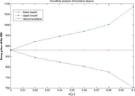
The dynamic relationship between hesitation degree and fuzzy prices of the CDS (k=0.5, λ=0.5)
| Time | 2013.06 | 2013.12 | 2014.06 | 2014.12 |
| Market data | 430 | 369 | 368 | 366 |
The actual derivatives market data (the datas come from the report of the international clearing bank)
| (κ, λ) | (0, 1) | (0.1, 0.9) | (0.2, 0.8) | (0.3, 0.7) | (0.4, 0.6) | (0.5, 0.5) |
| [257, 1603] | [361, 1483] | [465, 1362] | [569, 1242] | [672, 1121] | [776, 1001] |
Fuzzy prices of the CDS in different cut set levels
| (1.45, 1.55) | (1.40, 1.60) | (1.35, 1.65) | (1.30, 1.70) | (1.25, 1.75) | (1.20, 1.80) | |
| [1009, 1113] | [984, 1161] | [962, 1217] | [942, 1285] | [923, 1365] | [905, 1461] |
Fuzzy prices of the CDS in different fuzzy degree of external shocks (b1=c1=1.5)
| (0.45, 0.55) | (0.40, 0.60) | (0.35, 0.65) | (0.30, 0.70) | (0.25, 0.75) | (0.20, 0.80) | |
| [1419, 1698] | [1408, 1726] | [1398, 1753] | [1387, 1781] | [1376, 1808] | [1365, 1835] |
Fuzzy prices of the CDS in different fuzzy degree of internal contagion effect (b=c=0.5)
5. Conclusions
Due to the financial markets are always in volatility, the external shocks, such as the significant fluctuations of stock prices and market credit rating, may amplify the company’s default intensity, and even lead to defaults, then there may be default contagion between different companies, that is, counterparty credit risk is caused by market risk. Hence, in the management of counterparty credit risk, we should taking into account both the market risk and credit risk. Meanwhile, the external shocks and internal contagion effects on the company can not be observed, we can’t get the accurate size of the shocks. Therefore, based on the external shocks and internal contagion effects, we have proposed a new default intensity model with attenuation effects, and introduced the triangular intuitionistic fuzzy numbers into the CDS pricing modeling to describe the fuzziness and hesitation of the sensitivity coefficients of the default intensity, finally, through the simulation analysis, we obtained that, all kinds of fuzziness and hesitation of the market have significant impact on credit spreads, and a model result with a consideration of the fair price of CDS in a fuzzy random environment including a pure random environment result, this means a proper price range can offer the investors more flexible options and also make the model result more resemble the real market environment. However, there are still some deficiencies in this paper, for example, due to the limited market data, the model only through a simulation calculation to prove its effectiveness, and could not carry out the full empirical analysis, meanwhile, using a single fuzzy random variable is insufficient to accurately describe the fuzzy random characteristics of the derivatives market. Further research will include studies of the parameter estimation problem, that is, with the help of the price information obtained from the derivatives market, we will reconstruct the process of the price of fuzzy credit spreads in the risk neutral probability measure. Another possible extension of the study is robust control problem, in other words, the problem of how to obtain the fuzzy credit spreads with high stability.
Acknowledgements
The authors are very grateful to the anonymous reviewers for their insightful and constructive suggestions. The work was supported by the National Natural Science Foundation of China (No.71171051).
References
Cite this article
TY  - JOUR
AU  - Liang Wu
AU  - Ya-ming Zhuang
AU  - Wen Li
PY  - 2016
DA  - 2016/04/01
TI  - A New Default Intensity Model with Fuzziness and Hesitation
JO  - International Journal of Computational Intelligence Systems
SP  - 340
EP  - 350
VL  - 9
IS  - 2
SN  - 1875-6883
UR  - https://doi.org/10.1080/18756891.2016.1161345
DO  - 10.1080/18756891.2016.1161345
ID  - Wu2016
ER  -