
A Generic Preprocessing Optimization Methodology when Predicting Time-Series Data
- DOI
- 10.1080/18756891.2016.1204113How to use a DOI?
- Keywords
- Preprocessing Optimization Methodology; forecasting; Genetic Algorithms; Ant Colony Optimization
- Abstract
A general Methodology referred to as Daphne is introduced which is used to find optimum combinations of methods to preprocess and forecast for time-series datasets. The Daphne Optimization Methodology (DOM) is based on the idea of quantifying the effect of each method on the forecasting performance, and using this information as a distance in a directed graph. Two optimization algorithms, Genetic Algorithms and Ant Colony Optimization, were used for the materialization of the DOM. Results show that the DOM finds a near optimal solution in relatively less time than using the traditional optimization algorithms.
- Copyright
- © 2016. the authors. Co-published by Atlantis Press and Taylor & Francis
- Open Access
- This is an open access article under the CC BY-NC license (http://creativecommons.org/licences/by-nc/4.0/).
1. Introduction
In data-oriented analysis and modelling, data preprocessing (DP) is the most resource intensive phase. 1, 2 DP covers all computational steps that deal with raw data and lead to the final dataset which will be explored with the aid of data-mining computational intelligence (CI) algorithms. DP is often recommended in order to highlight relationships between members of the feature space, to create more uniform data in order to facilitate CI algorithm learning, and to meet algorithm requirements, avoiding computational problems. 3, 4
In Ref. 5 we have focused on the computational steps preceding the use of forecasting models. In the current paper we extend this approach by suggesting the Daphne Optimization Methodology (DOM), which is built to improve the preprocessing computational steps over time-series dataset, in terms of the performance of various forecasting algorithms applied to the output of the DOM. The order of the computational steps prior to the application of forecasting models, which define the optimization problem, are described in the Daphne Optimization Procedure (DOP).
The motivation for creating the DOM originated from the following question: Given a specific dataset with time stamped feature records, a set of data preprocessing algorithms and a set of forecasting algorithms, which combination of these algorithms leads to the best performance of the forecasting algorithms?
The DOM is evaluated in comparison to the traditional use of the optimization algorithms, Genetic Algorithms (GAs) and Ant Colony Optimization (ACO). The next four optimization algorithms have been used and evaluated for their optimization performance: 1) Traditional GA, 2) Traditional ACO, 3) Daphne-GA, and 4) Daphne-ACO. Each optimization algorithm was used to find solutions that lead to the best performances of the forecasting methods, when forecasting the daily mean concentration of respirable particles. These optimization algorithms were executed with different predefined execution parameters in order to evaluate their performance. The performance of the optimization algorithms was calculated in terms of best forecasting performance in minimum execution time. In addition, an exhaustive search of all solutions has been performed, for comparison.
The rest of the paper is structured as follows: Section 2 describes a) the optimization algorithms that were used by DOM, b) the methods that were used to deal with the problem of each computational step, c) the dataset that was used, and d) how the data was separated. Section 3 describes how the optimization problem was divided into discreet steps (that formulate a general procedure), and how the distance between different methods was calculated. Sections 4 describe the phases of DOM in detail. Sections 5 and 6 describe how the DOM was materialized by using the selected optimization algorithms, Genetic Algorithms and Ant Colony Optimization, respectively. Section 7 describes the evaluated models and the procedure that was performed in order to evaluate them. Section 8 describes the results of the work and discusses the basic findings of this study. Finally section 9 draws conclusions for DOM performance in comparison to the traditional use of the selected optimization algorithms.
2. Materials and Methods
In the optimization problem under study the initial dataset represents a knowledge pool that we would like to map in the best possible way, in order to facilitate the forecasting of the future state and behavior of the system that such a pool represents and describes. This requires a learning process that is well suited to the characteristics of CI-based evolution algorithms. For this reason we have selected to make use of two algorithms of this category, namely Genetic Algorithms and Ant Colony Optimization.
2.1. Genetic Algorithms
GAs are one of the well-known evolutionary algorithms (EAs) and were initially proposed and analyzed by Holland. 6, 7, 8 The GA is an optimization and search technique inspired by the theory of evolution and an understanding of biology and natural selection. 6, 7, 9, 10 The basic concept of GAs is to simulate the processes of natural systems necessary for evolution. As such they represent an intelligent exploitation of a random search within a defined search space, rendering them appropriate for an optimization problem such as the one addressed in our study.
2.2. Ant Colony Optimization
Dorigo et al. 11, 12 were inspired by the double bridge experiment 13, 14 to design the first ACO system, with an algorithm called Ant System (AS), which initially applied to the travelling salesman problem. An essential aspect of ACO is the indirect communication of the ants via pheromone (stigmergy). Ants deposit pheromone on the ground (environment) to mark their paths towards food sources. The pheromone traces can be detected by other ants and thus lead them to the food source. ACO exploits a similar mechanism for solving optimization problems. 15, 16
2.3. Fitness Function
The fitness function is the method of assigning a heuristic numerical estimate of quality (fitness) to a particular solution. 17, 18 In GAs, fitness evaluation provides feedback to the learning algorithm regarding which solution should have a higher probability of being allowed to procreate and which individuals should have a higher probability of being removed from the population. 6 In ACO, ants deposit a quantity of pheromone depending on the fitness of the solution. The quantity of pheromone’s deposition increases as fitness increases. For minimization problems, the fitness function usually approaches zero as the optimal value. For maximization problems, the fitness function usually approaches some upper boundary threshold as its optimal value. 18
2.4. Cross Validation
Cross validation (CV) is a popular method applied in order to evaluate the predictive performance of a statistical model. 19 In CV, the available dataset is divided into two segments, one is used to teach or train a model and the other is used to validate the performance of the model. There are several types of CV methods such as the Holdout method, k-fold, and leave-one-out. 20
K-fold CV divides the dataset into k (equal) subsets. Each one of the k subsets is used as the test set (i.e. the set against which the model performance is evaluated) and the other k-1 subsets are used as a training set. The k results from the folds (k times) are averaged for producing a single estimation. The advantage of this method is that the results are not influenced by the way the data are divided.
2.5. Arsenal of Methods
The DOP requires an arsenal of methods for each computational step. In this study a total of 40 methods were available for the DOP. Table 1 presents the methods that have been used for each computational step of the DOP. The reasons that lead us to select these methods are:
- •
The majority of them are included in Matlab’s libraries or have been published on the Matlab File Exchange website 21. Moreover, they have received positive reviews in terms of comments and ratings.
- •
| Computational Step | Methods |
|---|---|
| Step 1:Remove Outliers (Total: 11 methods) | Standard Deviation Criterion (i.e. removing all values that are more than 2 STD away from the mean) 24 |
| Robust Function Bisquare (Tukey’s biweight) 25 | |
| Robust Function Andrews 25 | |
| Robust Function Cauchy 25 | |
| Robust Function Fair 25 | |
| Robust Function Huber 25 | |
| Robust Function Logistic 25 | |
| Robust Function Ols (Ordinary least squares) 25 | |
| Robust Function Talwar 26 | |
| Robust Function Welsch 25, 27 | |
| Median Absolute Deviation (MAD) 23 | |
| Step 2: Handling of Missing Data (Total: 10 methods) | Interpolation algorithm Linear |
| Interpolation algorithm Linear with extrapolation | |
| Interpolation algorithm Piecewise 28 | |
| Interpolation algorithm Piecewise with extrapolation | |
| Interpolation algorithm Cubic 28 | |
| Interpolation algorithm Cubic with extrapolation | |
| Interpolation algorithm Spline 28 | |
| Interpolation algorithm Spline with extrapolation | |
| Interpolation algorithm Nearest 29 | |
| Interpolation algorithm Nearest with extrapolation | |
| Step 3: Smoothing Data (Total: 6 methods) | Moving Average |
| Local regression 1st degree polynomial model (lowess) 30, 31 | |
| Local regression 2nd degree polynomial model (loess) 32 | |
| Savitzky-Golay filter 33 | |
| A robust version of ‘lowess’ 30 | |
| A robust version of ‘loess’ 30 | |
| Step 4: Detrending Data (Total: 4 methods): | Constant detrending 22 |
| Straight (linear) detrending 22 | |
| Fit and remove a 2nd degree of polynomial curve 34 | |
| Hodrick-Prescott filter 35 | |
| Step 5: Feature Selection / Extraction (Total: 3 methods): | Factor Analysis 36, 37 |
| A simple feature selection based on the Covariance. Which selects the features with highest covariance (between the target variable) | |
| Principal Components Analysis (PCA), with variable explained criteria 38 | |
| Step 6: Forecasting (Total: 6 methods): | Linear Regression |
| Artificial Neural Networks, Feed Forward Back Propagation (FFBP) 39 | |
| Linear Neural Networks 40 | |
| Generalized Regression Neural Networks 41 | |
| Generalized linear model regression 42 | |
| Multivariate adaptive regression splines (MARS) 43 |
The methods used for each computational step of the DOP
Additional methods could be used for each computational step, but it would increase significantly the search space of the optimization problem. This would make it impossible to use the selected evaluation procedure, which is described in Section 7.
2.6. Data Presentation
The data used in this study consist of air quality observations made at the Agia Sofia monitoring station in Thessaloniki, Greece. Thessaloniki is the second largest city of Greece, and is characterized by a pronounced problem of air pollution, especially in terms of Particulate Matter (PM) and more specifically of respirable particles (PM10, i.e. particles of aerodynamic diameter small than 10µm). For this reason, the selected forecasting parameter of this study was the daily mean concentration of PM10.
The data consists of 1010 daily records for the years 2010 to 2012 (3 years) and includes a total of 12 parameters: 8 air pollutant parameters and 4 meteorological parameters. The air pollutant parameters were: 1) Daily mean concentration of Particulate Matter (PM10), 2) Daily maximum eight-hour running average concentration of Ozone, 3) Daily mean concentration of Ozone (O3), 4) Daily mean concentration of Nitrogen dioxide (NO2), 5) Daily mean concentration of Nitrogen oxides (NOX), 6) Daily mean concentration of Carbon monoxide (CO), 7) Daily maximum eight-hour running average concentration of CO, and 8) Daily mean concentration of Nitrogen monoxide (NO). The meteorological parameters were daily mean values of: 1) Relative Humidity (%), 2) Air Temperature (C), 3) Wind Speed (Km/h), and 4) Wind Direction (Degrees).
The air pollutant data were obtained from the European air quality database (AirBase) 44, and the meteorological data were obtained from the weather underground web site. 45
2.7. Data Separation
One of the most important parts of evaluating machine learning is to train the models on a training set that is separate and distinct from the test set, for which their modelling accuracy will be evaluated. If this part is not performed, it can result in models that do not generalize to unseen data.
The data in this study were separated into two datasets. The first 70% of the data (approximately, 2 years of daily records) were used in the training set, and the remaining 30% of the data (approximately, 1 year of daily records) were used in the test set. As an exception, in the Artificial Neural Network (ANN) models, the aforementioned 30% of the data was divided in two parts; the first 15% of the data were used in the test set, and the remaining 15% of the data were used for the validation set. The validation set is used by the ANNs to monitor the error during the training process, in order to stop the training when the network begins to overfit the data. 46
In addition the 10-Fold CV was used in order to measure the predictive performance of a statistical model. Fig. 1 shows a) how the data was separated and b) how the CV was performed on the data. The test set (and the validation set in the case of ANNs) was not included in the preprocessing steps in order to evaluate their contribution to the forecasting performance. As an exception, the replacement of missing values was performed on the test set (and validation set), for the cases where some forecasting methods cannot interpret them.
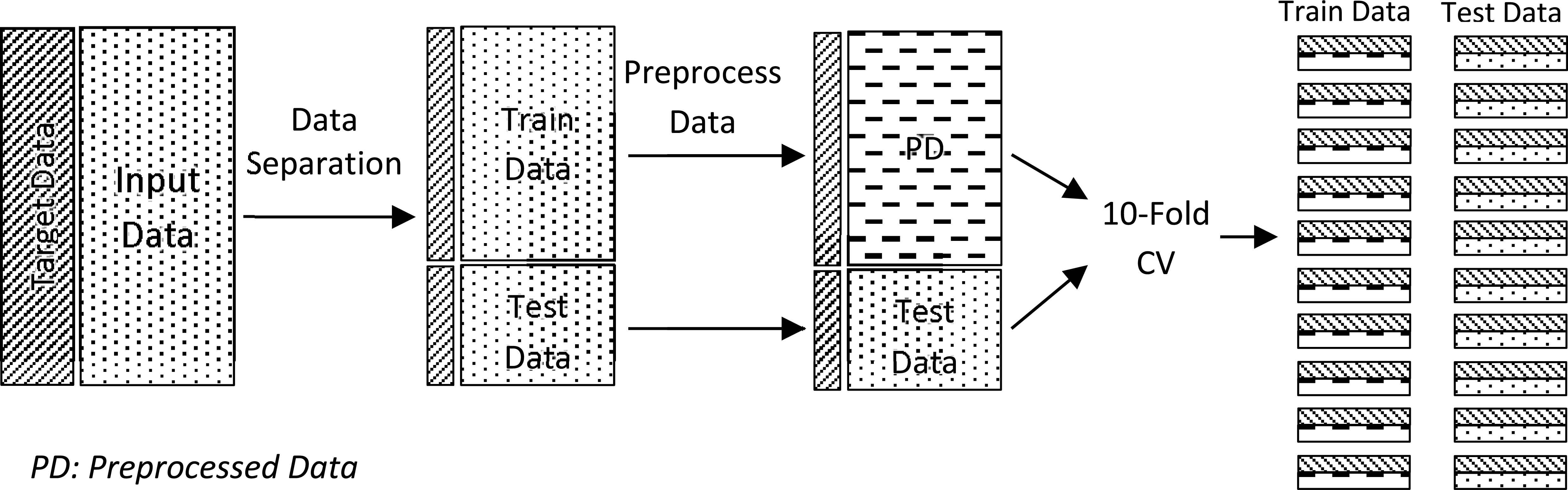
Data separation in the evaluation procedure
3. The Daphne Optimization Procedure
Although there are various approaches to DP in the literature, it is generally accepted that they include the following computational steps when applied prior to the application of forecasting models: 2, 47
- •
Identification and removal of outliers
- •
Dealing with the missing value problem
- •
Denoising-Smoothing of data
- •
Detrending
- •
Feature selection
- •
Forecasting
It should be emphasized that the forecasting step mentioned here is actually the testing step that evaluates the effectiveness of all previous preprocessing computational steps. On this basis, the DP efficiency is verified, and its results can then be used with various forecasting algorithms.
On this basis, the DOP describes the order in which to use the six aforementioned computational steps and define the optimization problem. Table 2 presents the computational steps, while Fig. 2 demonstrates the graphical structure of the DOP. Each computational step in DOP consists of a number of computational methods that can be applied to the data. At each computational step only one computational method is applied to the input data, to avoid redundancy (Fig. 2). This can be seen in Fig. 2 where the bold edges show a possible path. Steps 1, 3, 4 and 5 include also the option not to use any computational method. In the current paper the computational methods of the computational steps prior to the forecasting step, are referred to as preprocessing methods.
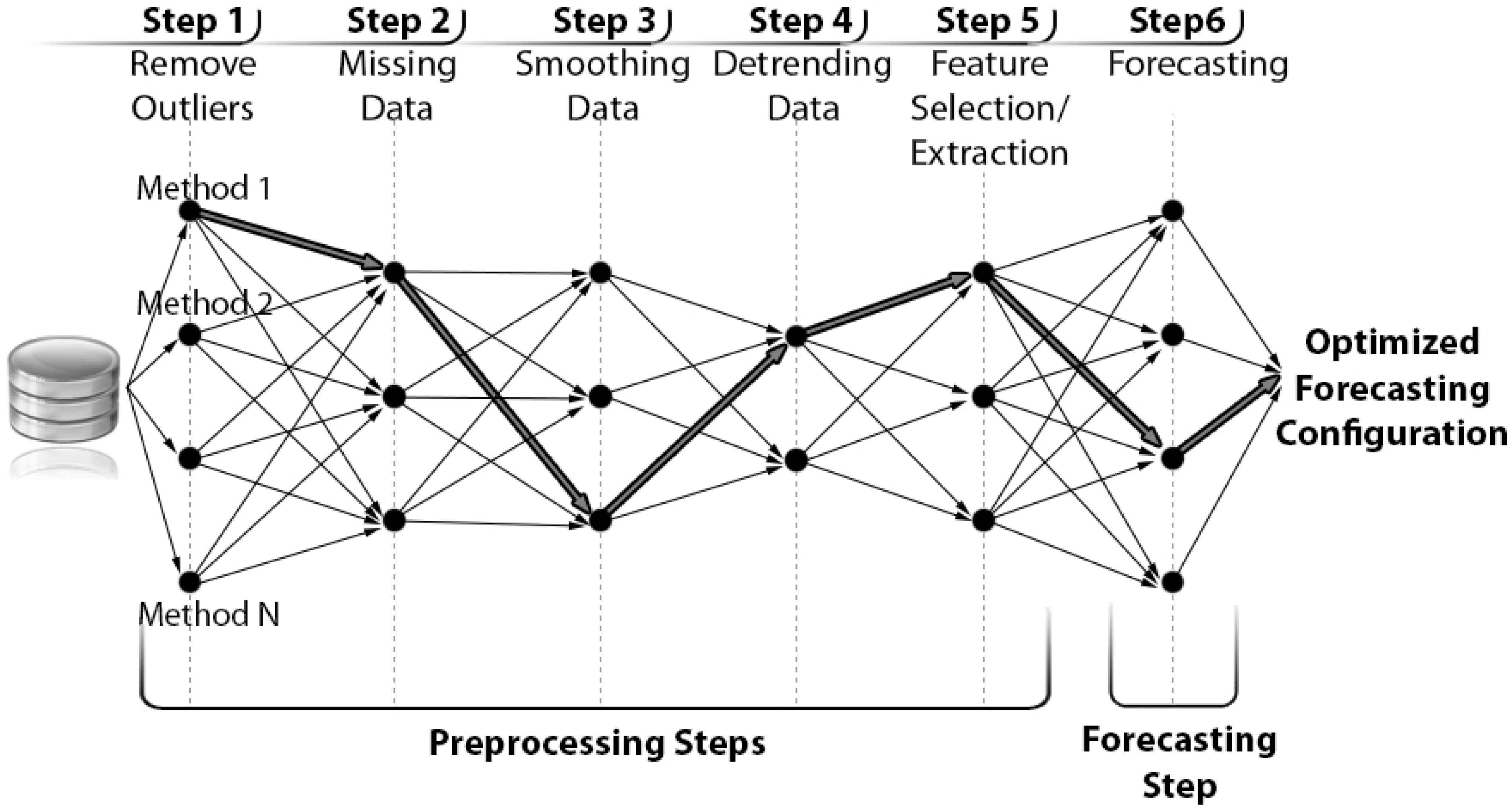
A graphical example of the DOP
| Computational Step | Name | Description |
|---|---|---|
| 1 | Remove Outliers | The outliers will be identified and removed from the data (will be treated as missing values) |
| 2 | Replace Missing Data | All missing values will be replaced by an estimated value |
| 3 | Smooth Data | A smoothing function will be used to remove noise |
| 4 | Detrend Data | Trends will be identified and removed from data |
| 5 | Feature Selection / Extraction | Input data will be reduced, either by selecting a subset of relevant features, or by reducing their dimensionality |
| 6 | Forecasting | A forecasting method will be used as the criterion to evaluate previous computational steps and thus lead to the final dataset |
The DOP computational steps
There are no algorithms that can select the computational method per step that optimizes the overall DP procedure, apart from the exhaustive search of all combinations of available computational methods. Our problem has the form of a longest path problem 48, with the following characteristics:
- (a)
the paths between DP methods are directed and simple (weighted edges), and
- (b)
only one method can be used per computational step.
In our case, we aim at finding the path with the best forecasting performance. Nevertheless, in order to accomplish this, we have to compute the distance (weights of the edges of the graph representing the optimization path) between the methods of the different computational steps, an issue addressed in the following section.
3.1. The Distance between Different Methods
To calculate the distance (D) or edge’s weights of the DOP graph, we have to apply those methods to the input data, one at a time, and calculate their individual forecasting performance. The basic idea of the weights is thus to represent the effect of each method on the forecasting performance. Fig. 3 presents an example of a distance calculation in the DOP graph. In this example, in order to calculate the distance D (1.2), method 1.2 (means: computational step 1, computational method of aforementioned step= 2) must be applied to the input data.
P(ma.c), is the forecasting performance, by using data which are preprocessed using method c of step a.
P(ma), is the vector of forecasting performances for all computational methods of step a.
P(ma.c,mb.d), is the forecasting performance, when using data which are preprocessed using method c of step a followed by method d of step b
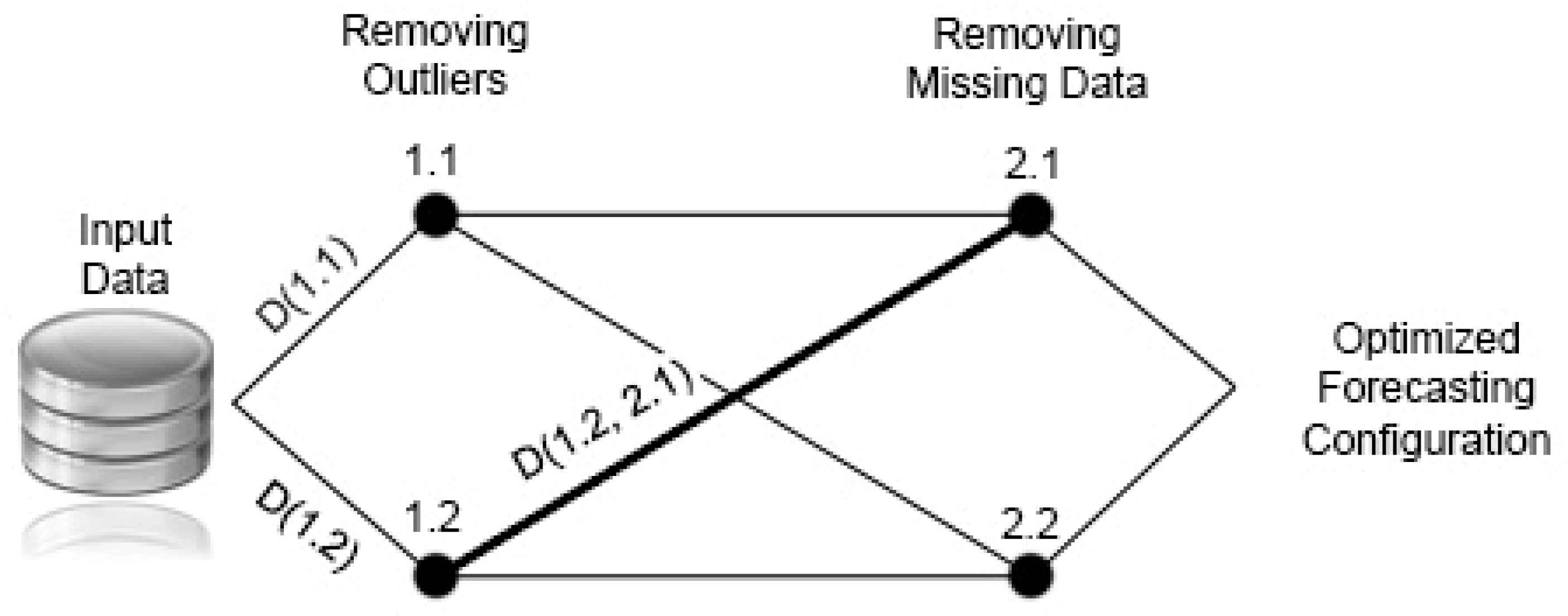
Distance calculation in DOP graph
The example presented in Fig. 4 demonstrates the calculation of the distance of the various computational methods in the DOP graph. Here we can see that methods 2.1 and 2.2 lead to a better forecasting performance, provided that method 1.1 was used in the previous computational step. In addition, method 2.1 has a negative effect on the forecasting performance in the case that method 1.2 was used in the previous step, while method 2.2 has no effect on the processing forecasting performance, when method 1.2 is preceding.
D(1.1) = P(1.1) – min(P(1)) = 0.90 – 0.90 = 0
D(1.2) = P(1.2) – min(P(1)) = 0.91 – 0.90 = 0.1
D(1.1, 2.1) = P(1.1, 2.1) – P(1.1) = 0.93 – 0.90 = 0.03
D(1.1, 2.2) = P(1.1, 2.2) – P(1.1) = 0.92 – 0.90 = 0.02
D(1.2, 2.1) = P(1.2, 2.1) – P(1.2) = 0.85 – 0.91 = -0.06
D(1.2, 2.2) = P(1.2, 2.2) – P(1.2) = 0.91 – 0.91 = 0
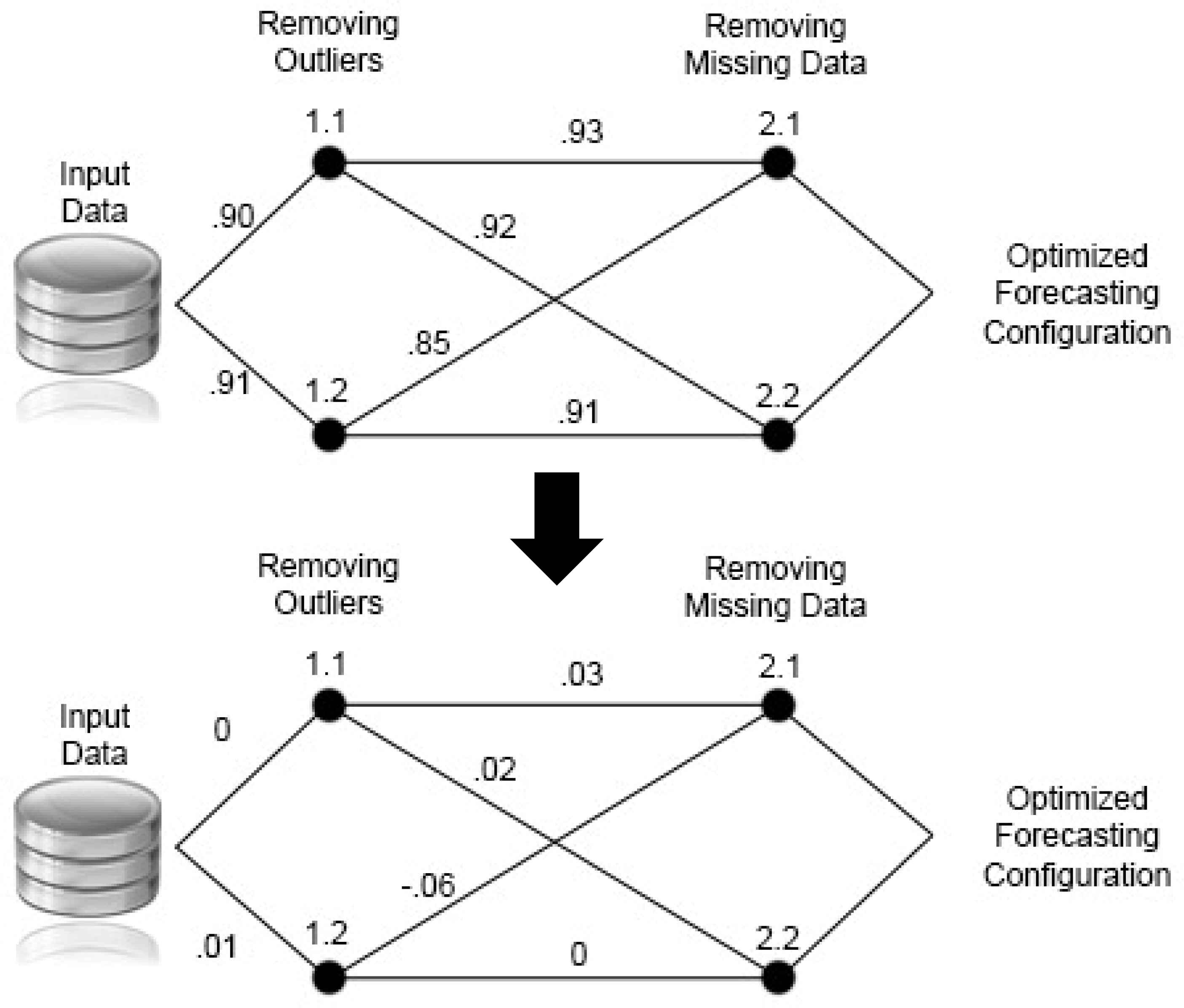
Example of a DOP graph, a) with forecasting performance (on the top) and b) the calculated distance (on the bottom)
For the case where the methods are skipped from the evaluation procedure, their distances have been set to zero (i.e. no effect on the forecasting performance).
4. The Daphne Optimization Methodology
The DOM initiates the phases in the following order.
Phase 1. The performance of each one of the forecasting methods is calculated without using any data preprocessing method. (In cases where the forecasting methods have special requirements, certain computational steps are followed: for example, ANNs cannot interpret missing values, thus a preprocessing method to deal with missing values must be used.)
Phase 2. Calculate the performance of each one of the forecasting methods by using only one data preprocessing method for all computational steps. This is an optional phase, as it can be part of the optimization algorithm that will be used for the final selection of the best possible combination of optimization steps. In our study, we included this phase in the two optimization algorithms employed, i.e. GA and ACO.
Phase 3. Get the next feasible combination of computational methods to evaluate, by taking into consideration the distance-effect of each method. The formulation of the next feasible combination depends on the optimization algorithm employed. In the next sections, we describe the modifications necessary for GA and ACO to be applied in the frame of the DOM.
Phase 4. Apply the combination of computational methods to the input data and calculate the distances. For the intermediate computational steps of the DOP (Step 1 to Step 5, of Fig. 2),the Linear Regression method can be used to calculate the forecasting performance for the distance calculations. Linear Regression can be used for this purpose in order to provide a quick estimation of the forecasting performance. The output of each preprocessing method of the combination can be stored temporarily (as cache) in order to be reused in different combinations of preprocessing methods. This will reduce the processing time but will increase the necessary disk space and memory. If this mechanism is used, a search for existing cached output data must be carried out in order to facilitate its reuse and also any unsaved preprocessed output data must be saved temporarily (cached).
Phase 5. If the terminal conditions are reached the process stops, otherwise Phases 3 to 5 are to be repeated. The next two terminal condition were used in all optimization algorithms:
- 1.
The maximum number of iterations (in GA parlance referred to as generations) has been reached.
- 2.
The fitness function does not change over successive iterations. For that purpose, the average changes in fitness between successive iterations of Eq. (3) must be calculated. When the 3-iterations moving average of |fΔ| is equal or lower than a preset change tolerance threshold, the optimization procedure stops.
Where,
fΔ is the average change in the fitness from one iteration to the next.
K is the total number of iterations elapsed.
- 1.
5. DOM for Genetic Algorithms
In order to use GAs for the materialization of the DOM, we need to generate an initial population of solutions, which, in this case, are possible combinations of methods for the computational steps. In addition, we need to define the crossover mechanism to be used when combining GA solutions in order to produce the (better) solutions of the next generation. For this reason, two parts of the “traditional” GAs have been modified. In the first modification, a function that generates initial populations with a) feasible and b) unique solutions was created. In our optimization problem a solution is a combination of methods (one for each DOP step). The initial solutions did not include any preprocessing technique, except from a method to replace the missing values, which was selected at random. This function will be applied during Phase 1 of the DOM.
In the second modification, the Daphne Uniform Crossover (DUC) method was created in order to use the calculated distance-effect of each method and perform targeted genome crossovers. This method is a modified version of the Uniform Crossover which uses the distance between the different methods to perform crossover. The advantage of DUC method is that it swaps the genomes on the basis of a probability depending on the distance-effect of each method, and not at random by using a constant probability (mixing rate).
5.1. The Daphne Uniform Crossover
In the traditional uniform crossover the loci positions in the genome are selected at random (using a constant probability referred to as the mixing rate) and the specific genes are exchanged. The DUC selects the loci positions in the genome from a variable probability depending on the distance-effect of each method. In this way the DUC controls the genetic diversity.
The DUC can be used in many different ways, in order to compute the exchange rate for each gene. In the following section we present three different ways to compute the exchange rate for each gene from the distance-effect.
Method-1 crossover: Exchange the “bad” genes
In this method of exchange, the loci positions with “bad” genes (i.e. the genes with lower distance) have higher probability of being exchanged. The idea is to keep the “good” genes, which will probably be consecutive, and thus, the behavior that evolves as patterns in the population will be preserved. This is not possible in the traditional uniform crossover. In addition, by exchanging the loci positions of the “bad” genes of both parents, it is expected that the fitness of the offspring will increase. The exchange probability of each loci position varies around a constant mixing rate, as can be seen in Eq. (4).
Where,
i, is the ith loci position
D, in the distance for each loci position in the genome
The exchange rate can be calculated by using Eq. (4) for each parent, and the maximum value is kept for each loci position.
Method-2 crossover: Pass the “good” genes to the first child
Zajonc formulated 49 and applied 50 the confluence theory to explain the relationships between birth order and intellectual development, arguing that later-born children tend to be less intelligent than earlier-born children. Method-2 of selecting the loci positions to be exchanged was inspired by Zajonc’s work. Method-2 exchanges the loci positions where the second child’s distance is greater than the first’s. The exchange rate in these cases has a value of 1, and in all others have a value of 0. In this way the first child will get all the “good” genes and is expected to show an increase its fitness. It should be noted that in this type a constant mixing rate is not needed.
Method-3 crossover: A combination of Method-1 and Method-2
This crossover method combines the previous two methods in order to exchange the parent’s genes. First, Method-2 is used in order for the first child to get all the “good” genes; in the cases where the second child’s distance is greater than the first’s. In the cases in which the first child has already all the good genes (and no exchange will be performed by Method-2), the Method-1 was used. By using Method-1 in these cases, we will prevent premature convergence in the GA.
6. DOM for Ant Colony Optimization
The ACO is very close to our methodology because the ants travel through a path towards their destination (food source). The application of the ACO meta-heuristic to the traveling salesman problem 51 is similar to our problem. The main differences are: a) our problem has to find the longest path (not the minimum), and b) our path is not a Hamiltonian circuit.
In order to compute the ant-routing table, Eq. (5) was used, where D(ma.c,mb.d) is the distance between methods c (of step a) and d (of step b), as shown in Eq. (6). The distance of each edge (methods c and d) of the path has been calculated with Eq. (1) and Eq. (2), with a value range of [-1, 1]. In Eq. (6), the value 1 was added, in order to produce a positive heuristic value in the range of [0, 2]. Thus, the longer the distance between two methods, the higher the local heuristic value.
Where,
τa.c,b.d is the strength of the pheromone,
ηa.c,b.d is visibility, i.e. a simple heuristic used in deciding which edge is the most attractive to be visited next
alpha is a constant affecting the strength of the pheromone
beta: a constant affecting visibility
Where,
Ni is the set of all the neighbor nodes of node i.
Each ant k deposits a quantity of pheromone Δτk(t) on each connection that it has used. The Δτk(t) is the forecasting performance of the model, by ant k in iteration t, as shown in Eq. (7).
Where,
m is the number of ants (is maintained constant in all iterations)
In order to avoid convergence to a locally optimal solution, pheromone evaporation is performed. In pheromone evaporation, the arc’s pheromone strength is updated as follows: τnew = (1 − ρ)τold, where ρ ∈ (0, 1] controls the speed of pheromone decay. 52
The probability
Where,
7. DOM Evaluation
The DOM was applied together with two optimization algorithms (GA and ACO). As a result the next four optimization algorithms have been used and evaluated for their optimization performance:
- (i)
Traditional GA
- (ii)
Traditional ACO
- (iii)
Daphne-GA, and
- (iv)
Daphne-ACO.
The evaluation was performed in terms of best forecasting performance in minimum execution time. By the term “traditional” we mean the use of the optimization algorithms in their original form. In the earliest genetic algorithms (traditional), the related research on Holland’s original GA 53 usually maintains a single population of potential solutions to a problem and uses a single crossover operator and a single mutation operator to produce successive generations. 54, 55, 56 For the case of the traditional ACO the Ref. 57 meta-heuristic was used, which models the behavior of a group of real ant colonies to rapidly find the shortest path between food sources and nests. 58
For comparison, several (existing) methods for each step of the GA were used. Table 3 shows a) the methods that have been used for each step of the GA, and b) the design parameters of the GAs. This table includes the important decisions that factor into the design of the GAs. 17
| Method or Parameter | |
|---|---|
| Selection (of parents) | Double Tournament Selection, without replacement (the same parent cannot be selected twice) |
| Roulette Wheel Selection | |
| Rank Selection | |
| Crossover Parents (produce offspring) | Uniform Crossover |
| Double Point Crossover | |
| Daphne Uniform Crossover | |
| Mutation | Uniform Mutation |
| Elite offspring | One elite offspring |
| Data structure (representation) | Real values |
| Fitness Function | Sugeno Forecasting Performance Index (FPIs) 59 |
The methods that have been used for each step of the GA and the design parameters of the GAs
In addition, in order to have accurate evaluation results an exhaustive search of all combinations of data preprocessing methods and forecasting methods (solutions) has been performed, for comparison. For the selected number of methods per computational step (Table 1), the exhaustive search equates to the execution of 100,800 different solutions (all possible combinations). The number of methods per computational step was selected in such a manner that would result in a limited search space where the exhaustive search could be used. In addition, a relatively small dataset (3-years of daily values) was selected for the same purpose.
Tables 4 and 5, show the investigated optimization algorithms models, for GA and ACO respectively. These optimization algorithms models can be used with different predefined execution parameters, which will affect their results (in performance and execution time). In this study, the optimization algorithms models have been executed with the predefined execution parameters of Table 6. Each execution, for the combination of optimization algorithms and different parameters, was repeated 10-times and the performance criteria was calculated from the average of those repeated executions. This was performed in order to produce reliable results, because of the heuristic nature of the optimization algorithms.
| # | GA Model Name | Crossover | Selection |
|---|---|---|---|
| 1 | DDO (Traditional GA) | Double-Point | Double Tournament |
| 2 | DRA (Traditional GA) | Double-Point | Rank |
| 3 | DRO (Traditional GA) | Double-Point | Roulette Wheel |
| 4 | UDO (Traditional GA) | Uniform | Double Tournament |
| 5 | URA (Traditional GA) | Uniform | Rank |
| 6 | URO (Traditional GA) | Uniform | Roulette Wheel |
| 7 | D-UDO (Daphne-GA) | DUC | Double Tournament |
| 8 | D-URA (Daphne-GA) | DUC | Rank |
| 9 | D-URO (Daphne-GA) | DUC | Roulette Wheel |
The investigated GA models
| # | ACO algorithm Model | Description |
|---|---|---|
| 1 | Traditional ACO | Using only the pheromone trails to guide the ants. |
| 2 | Daphne ACO | Using a local heuristic value depending on the calculated distance, and the pheromone trails to guide the ants. |
The investigated ACO algorithm models
| Optimization Algorithm | Parameter | Value(s) |
|---|---|---|
| GA | Crossover Rate | 0.2, 0.3, 0.5 |
| Mutation Rate | 0.05, 0.1, 0.2 | |
| Tournament Selection Size (TSS) | 3, 5, 8 | |
| Exchange Method | Method-1, Method-2, Method-3 | |
| ACO | Alpha (α) | 0.5, 0.75, 1 |
| Beta (β) | 1, 2.5, 5, 7.5, 10 | |
| rho (ρ) | 0.25, 0.5, 0.75 |
The execution parameters of the optimization algorithms models
7.1. The Optimization Performance Score
The criteria to compare the performance of each optimization algorithm’s execution were a) the best forecasting performance, and b) the execution time (speed). The goal of the optimization algorithms was to find a forecasting performance (that is close to the best) in a relatively short time period. In order to compare the performance of an optimization algorithm’s execution (e) with the performance of the other optimization algorithms executions, the Performance Score (PScore) as defined in eq. (9) was used. The performance criteria were firstly normalized by using feature scaling to standardize their range. The simplest method of feature scaling is to rescale the range of the variables to the range [0, 1] (Eq. (10) and Eq. (12)). The lower the PScore value, the higher the overall performance of the optimization algorithm.
Where,
e, is an optimization algorithm’s execution
The forecasting performance (the fitness function in GA) was calculated by using the Sugeno Forecasting Performance Index (FPIs) as proposed in Ref. 59. DOM is not restricted in the use of the FPIs as a forecasting performance method, but it can be used with other methods such as: Index of Agreement (dr) 60, 61 or Coefficient of Determination (r2).
8. Results and Discussion
The exhaustive search equates to the execution of 100,800 different models (all possible combinations). The time needed to execute all possible models was approximately 13 days, when using a personal computer, with an Intel(R) Core(TM)2 Quad CPU Q6600 @ 2.40GHz CPU (with Average CPU Mark: 2991) 62, and 4GByte RAM. The use of the exhaustive search helped a) to evaluate the results of the optimization accurately, and b) enables to study the search space of the problem. Fig. 5 shows the percentage of the models for each forecasting performance group. From Fig. 5 we can see that the highest performance of all models for the specific dataset used in this study is 0.5. In general this is not a very good forecasting performance, but its improvement was not a goal of this study. In addition, we can see that 3.7% of these models provide the best possible results (for the studied models), i.e. a performance between 0.4 and 0.5. The optimization algorithms would try to find the models corresponding to this 3.7%.
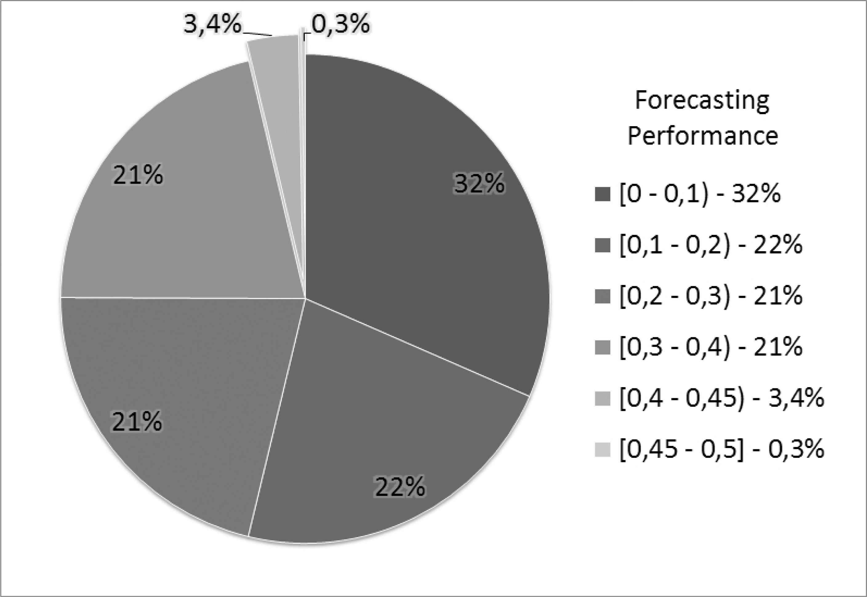
The percentage of the models for each forecasting performance group
Table 7 shows the ten best GA Models (from a total of 72 models) in terms of PScore. From Table 7 we can see that 90% of those models used the Double Tournament Selection method, with a TSS value 8. In addition, 70% of those models use a mutation rate value of 0.1. From Table 7, it is clear that the models with the highest PScore (50% of these models) used the DOM. The difference between the best model using DOM (1st model), compared to the best model not using DOM (4th model) was 2% PScore.
| GA Model | Crossover | Mutation | TSS | Exchange Method | Time (mm:ss) | Best Performance | PScore |
|---|---|---|---|---|---|---|---|
| D-UDO | 0.2 | 0.1 | 8 | Method-3 | 14:29 | 0,47 | 0,36 |
| D-UDO | 0.5 | 0.05 | 8 | Method-2 | 08:27 | 0,45 | 0,37 |
| D-UDO | 0.2 | 0.1 | 8 | Method-3 | 15:06 | 0,47 | 0,38 |
| UDO | 0.3 | 0.1 | 8 | - | 15:27 | 0,47 | 0,38 |
| DDO | 0.5 | 0.05 | 8 | - | 09:09 | 0,45 | 0,39 |
| DDO | 0.3 | 0.1 | 8 | - | 12:51 | 0,46 | 0,40 |
| D-UDO | 0.5 | 0.1 | 8 | - | 16:05 | 0,47 | 0,40 |
| DDO | 0.5 | 0.1 | 8 | - | 16:08 | 0,47 | 0,40 |
| URO | 0.5 | 0.05 | 8 | - | 13:21 | 0,46 | 0,41 |
| D-UDO | 0.5 | 0.1 | 8 | Type-2 | 16:41 | 0,47 | 0,42 |
The ten best GA Models in terms of the PScore
Table 8 shows the ten best ACO Models (from a total of 48 models) in terms of PScore. From Table 8 we can see that a) 60% of those models use an Alpha (α) value 0.5, b) 60% use rho (ρ) value 0.5. From Table 8, it is clear that the models with the highest PScore (70% of these models) use the DOM. The difference between the best model using DOM (1st model), compared to the best model not using DOM (5th model) was 6% PScore.
| ACO Model | Alpha (α) | Beta (β) | rho (ρ) | Time (mm:ss) | Best Performance | PScore |
|---|---|---|---|---|---|---|
| Daphne ACO | 0,5 | 7,5 | 0,5 | 20:23 | 0,49 | 0,41 |
| Daphne ACO | 0,5 | 10 | 0,5 | 21:20 | 0,49 | 0,43 |
| Daphne ACO | 0,75 | 5 | 0,5 | 21:26 | 0,49 | 0,43 |
| Daphne ACO | 1 | 2,5 | 0,5 | 22:46 | 0,49 | 0,47 |
| Traditional ACO | 0,5 | 0 | 0,25 | 15:12 | 0,47 | 0,47 |
| Daphne ACO | 0,5 | 5 | 0,5 | 19:21 | 0,48 | 0,48 |
| Daphne ACO | 0,5 | 1 | 0,25 | 19:42 | 0,48 | 0,49 |
| Traditional ACO | 0,75 | 0 | 0,5 | 08:29 | 0,45 | 0,50 |
| Daphne ACO | 0,5 | 7,5 | 0,25 | 20:04 | 0,48 | 0,50 |
| Traditional ACO | 1 | 0 | 0,75 | 04:50 | 0,44 | 0,50 |
The ten best ACO Models in terms of the PScore
In order to compare the results of the GA models with the results of the ACO models, the PScore values were calculated from both. From this calculation, we have seen that the best ACO model (of Table 8) is 3% better (in PScore) comparted to the best GA model (of Table 7). By comparing the results of the exhaustive search with the results of the optimization algorithms, the superiority of the optimization algorithms over the exhaustive search is evident. The optimization algorithms needed approximately 0.1% of the total time that was necessary for the exhaustive search, in order to find a near optimal solution (in terms of performance). These solutions were in the group of the best solutions (0.3% of the total search space).
9. Conclusions
In order to perform forecasts for time-series data, a combination (chain) of computational methods is employed (including the forecasting method). The selection of these methods is a very difficult but important task because it influences the forecasting performance. In this study, a general optimization methodology (referred to as Daphne) is introduced and evaluated in order to select the appropriate combination of methods to forecast time-series data.
The Daphne Optimization Methodology (DOM) is based on the idea of measuring the effect of each method on the forecasting performance, and using it as a distance in a directed graph. This graph represents all possible combinations of methods, which are grouped in six steps. Each step deals with a specific problem (e.g. remove outliers) and consists of a number of methods for the problem of each step. In addition, we have described two paradigmatic implementations together with Genetic Algorithms (GAs) and Ant Colony Optimization (ACO). The DOM is a general methodology, thus, it could be applied together with optimization algorithms (GA and ACO) in a different manner. For example, in the case of GAs, it could be used to create a driven mutation by the distance-effect of each method.
The DOM was applied and evaluated in the two aforementioned optimization algorithms: GAs and ACO. The evaluation procedure included comparisons with the traditional use of the optimization algorithms and with the exhaustive search.
Results show that the DOM has 2% and 6% better PScore, compared to the traditional use of the optimization algorithms, when using GA and ACO respectively. In addition, we have seen that the DOM provides 3% better PScore if it is used in the ACO, instead of in the GA. Thus, the DOM finds a solution (combination of preprocessing and forecasting methods) which is near the optimal in comparatively shorter time than with the traditional use of the optimization algorithms. This has the potential to be very helpful in “real” world problems, where commonly the search space is very large.
References
Cite this article
TY  - JOUR
AU  - Ioannis Kyriakidis
AU  - Kostas Karatzas
AU  - Andrew Ware
AU  - George Papadourakis
PY  - 2016
DA  - 2016/08/01
TI  - A Generic Preprocessing Optimization Methodology when Predicting Time-Series Data
JO  - International Journal of Computational Intelligence Systems
SP  - 638
EP  - 651
VL  - 9
IS  - 4
SN  - 1875-6883
UR  - https://doi.org/10.1080/18756891.2016.1204113
DO  - 10.1080/18756891.2016.1204113
ID  - Kyriakidis2016
ER  -