
Modified Black Hole Algorithm with Genetic Operators
- DOI
- 10.1080/18756891.2016.1204114How to use a DOI?
- Keywords
- Black Hole; Nature-inspired optimization; Metaheuristic algorithm; Benchmarking
- Abstract
In this paper, a modified version of nature-inspired optimization algorithm called Black Hole has been proposed. The proposed algorithm is population based and consists of genetic algorithm operators in order to improve optimization results. The proposed method enhances Black Hole algorithm performance by searching space with more diversity. The modified Black Hole algorithm has been applied to a well-known benchmark. The experimental results show that the modified Black Hole algorithm outperforms compared to some prominent optimization algorithms.
- Copyright
- © 2016. the authors. Co-published by Atlantis Press and Taylor & Francis
- Open Access
- This is an open access article under the CC BY-NC license (http://creativecommons.org/licences/by-nc/4.0/).
1. Introduction
Optimization problems have become a major field of interest for researchers in different propensities, and created an immense bunch of movement widely used in engineering applications. Due to complexity and nonlinearity of many engineering optimization problems, classic optimization approaches may tend to fail. Nature and bio inspired algorithms seem superior to their classic counterparts and have found specific places between the newfangled algorithms [1]. The effectiveness of these algorithms had been proven in many fields such as industry, hardware design, urban design, routing, image processing, project scheduling, Controller design, robots path planning, data clustering and etc. [2]
The Black Hole (BH) Algorithm is one of the optimization techniques inspired by the behavior of the real black holes. The black hole terminology is used for the first time in [3] to improve the convergence rate and efficiency of the PSO algorithm. Then, a new simple version of the BH algorithm was proposed in [4] for data clustering. In recent years, the BH algorithm and its modified versions have been used to solve optimization and engineering problems [5–18].
The aim of this paper is to cope drawbacks of the BH algorithm proposed in [4] such as getting trapped in local minima, and to provide the ability to solve both high and low dimensional problems. For this purpose, a modified Black Hole (MBH) algorithm is proposed in which the genetic programming and swarm intelligence has been employed concurrently to solve optimization problems. At each iteration, a particle with the best cost named as the Black Hole, and other particles called stars start moving towards the black hole with a random generated angle to cover the search space and find the best local minima. Similar to real black hole phenomena, a star is swallowed by the black hole if its distance to the black hole reaches the minimum. Also, the genetic operators called crossover and mutation are applied to the obtained space in order to improve the particles cost. The main modifications are as follows:
In standard Black Hole Algorithm, stars move directly toward to the black hole. But, in the proposed algorithm, stars move toward to the black hole with a restricted angle between −π/4 and +π/4, so the search space has been enlarged. The swallowing formula is changed to avoid the loss of stars close to global optimum when there are a lot of local optimums. The random numbers are selected between 0 and 2. Therefore, the proposed algorithm is able to scour the area around the black hole on both sides to find the best probable optimum. Some genetic algorithm operators (mutation and crossover) have been used in the proposed algorithm. The genetic operators are applied to improve the particles cost.
The rest of this paper is organized as follows: the black hole phenomena and standard optimization algorithm are presented in section 2. Section 3 describes the proposed MBH algorithm. A detailed comparison of the MBH algorithm and some prominent optimization algorithms are given in section 4. The paper is concluded in section 5.
2. Standard Black Hole Optimization Algorithm
A black hole is a geometrically defined region of space-time exhibiting such strong gravitational effects that nothing, including particles and electromagnetic radiation such as light, can escape from inside it [19]. The theory of a star becoming invisible was formulated by John Michell and Pierre Laplace in the eighteens-century. Then, John Wheeler named the mass collapsing phenomenon as a black hole in 1967 [4].
The size of a black hole, determined by the radius of event horizon or Schwarzschild radius, is roughly proportional to the mass M through
The BH algorithm is inspired by the behavior of real black holes. Like other population-based optimization algorithms, the stars as a randomly generated population of candidate solutions are placed in the search space. The movement of stars towards the black hole is formulated as follows [4]:
3. Proposed Modified Black Hole Algorithm (MBH)
Flowchart of the proposed modified black hole algorithm (MBH) is shown in Fig. 1. As noted, the modified black hole is a population-based optimization algorithm. A random population is generated and values of the cost function are calculated for all candidate solutions. Afterwards, exploration and exploitation sections are employed to analyze the search space, yet with the minimum computational efforts to reach the best point, independent of either being the minimum or the maximum. First, the random population is distributed in the search space. Then, the point with the lowest cost among others is picked to be the black hole, while the others are known as the stars. As in real black hole, due to its particular characteristics, the air converges at the ground level and all the stars try to reach the black hole. Here, stars with high costs are also gravitated to the black hole. A detailed and fully explained description of this procedure is discussed in section 3.2. At the end of each iteration, the mutation and crossover operators are also applied to the stars in order to improve the performance.
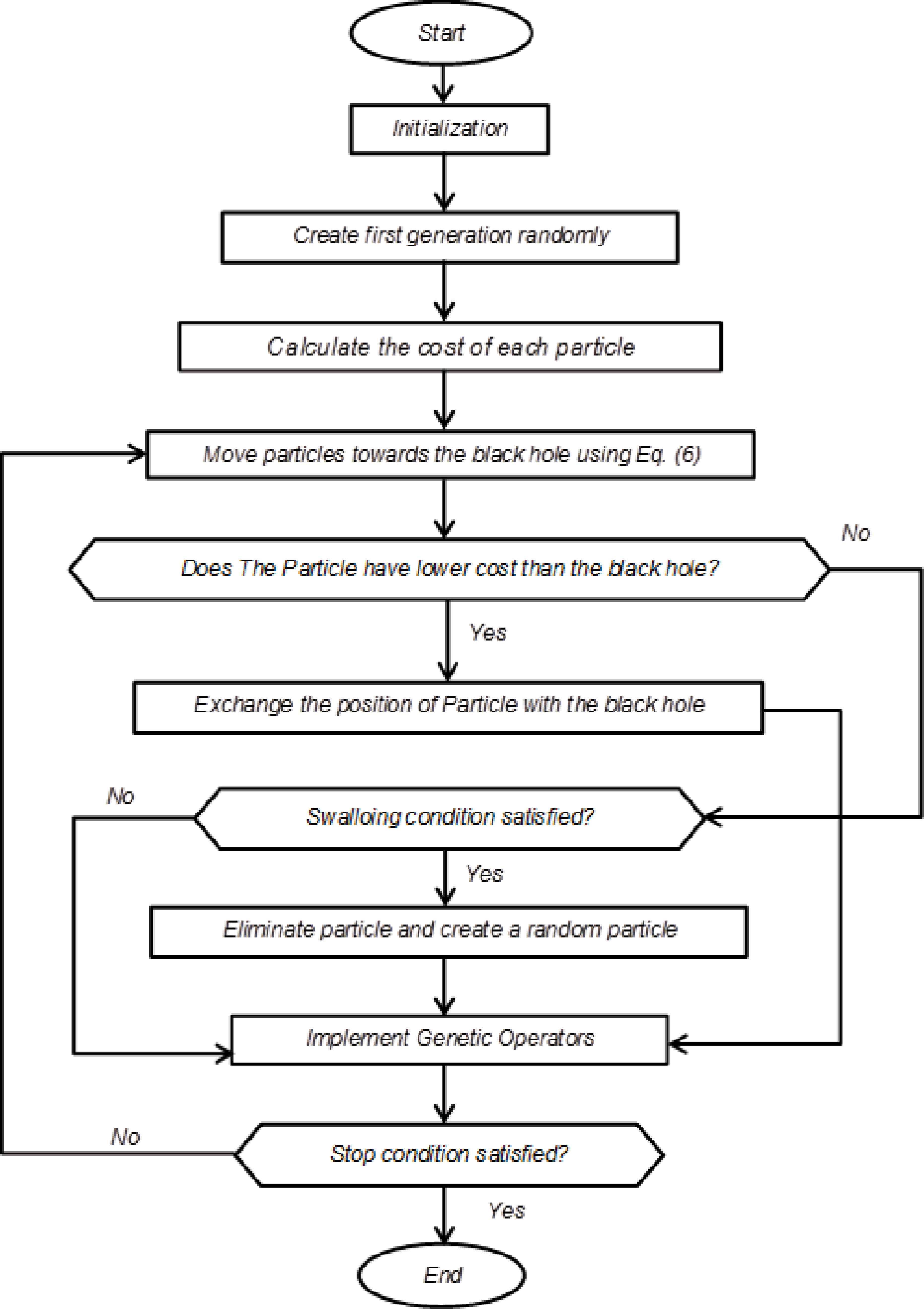
Flowchart of Modified Black Hole Algorithm.
3.1. Creating initial stars
As it is conventional in evolutionary algorithms, the whole information of each particle is stored in an array. This array is known as “particle position”, “chromosome”, and “habitat” in PSO [20,21], GA [22], and CS [23] algorithms, respectively. Here, it is known as: “star position”. The star position is a 1×Nvar matrix in solving an Nvar-dimensional problem. This matrix is defined as Eq. (4) :
All elements of this matrix are of floating point digit type. The cost of the point in space is obtained by applying the cost function over the point. This function is defined as:
At the first step of the optimization, Nvar stars are generated and distributed in the space randomly. The star with the most desirable cost is considered to be the black hole.
3.2. Moving stars towards the black hole
Following the aforementioned steps, the algorithm should make the stars move towards the black hole. This movement can be formulated as follows:
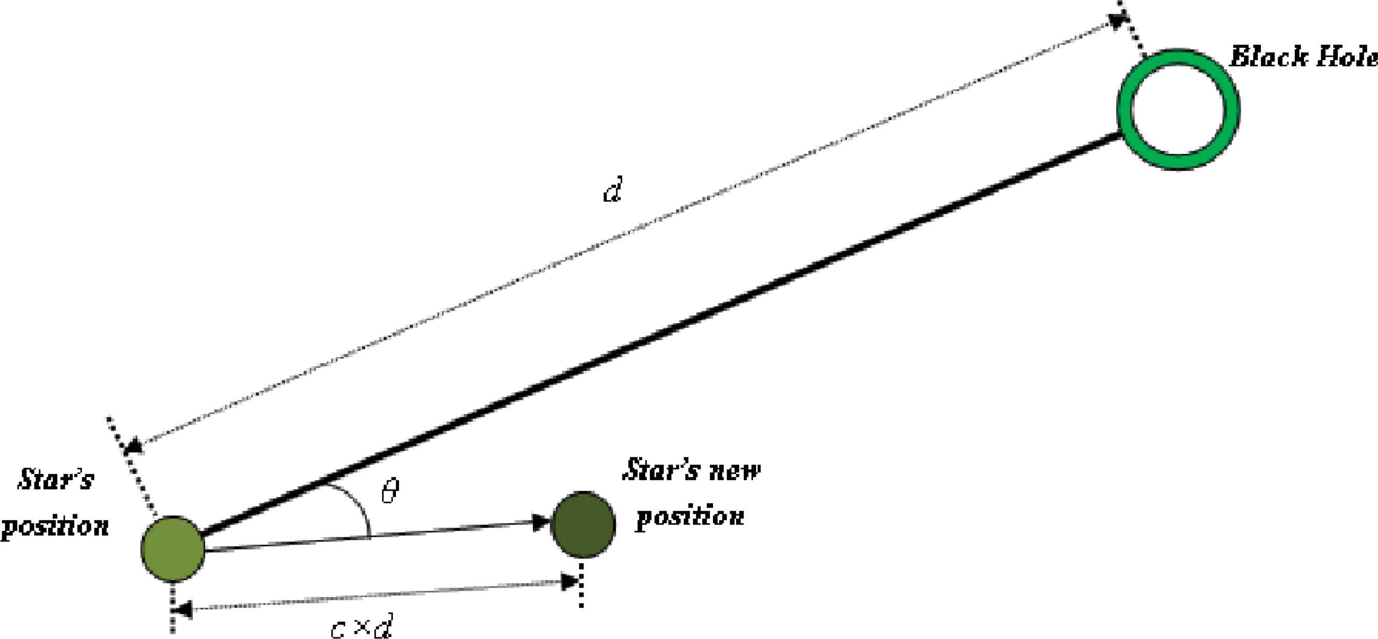
Moving particles (stars) towards the black hole.
After propelling stars towards the black hole, location of a star and the black hole are swapped, only if the assessed particle cost gets better than the previously selected black hole. In other words, particle is named as the new black hole and the previous black hole is known as the particle. Also, the other particles start to move towards the new black hole as shown in Fig. 3.
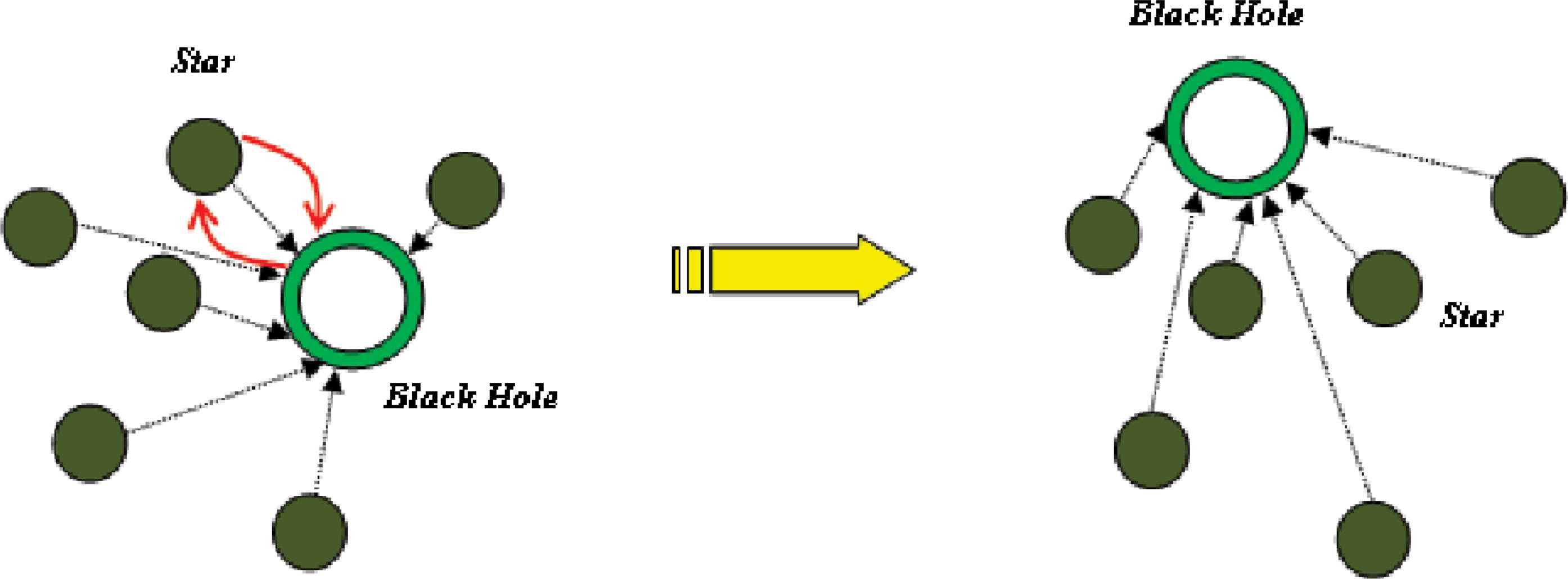
Exchanging position of a star and black hole when the star presents a more suitable cost.
3.3. Stars swallowing
In a real black hole phenomenon, when the particles reach the particular distance to black hole, they are gravitated and swallowed. The proposed method is also inspired by this procedure, in which, if a particle exceeds the minimum distance to the black hole, it will be swallowed and a new particle will be generated in the search space randomly. This distance can be defined as in Eq. (7) :
3.4. Limiting stars position
In some cases, stars are placed in a position where the movement towards black hole leads a particular star to be egressed from the search space. As a result, undesirable solutions may be generated. Hence, Eq. (8) is employed to restrict the particle probable positions in the search space frame.
3.5. Implementing mutation and crossover operators
The mutation and crossover operators are applied in order to meliorate the algorithm performance, if there is no improvement in results after 10% of total continual iterations. The first step of genetic operators section is parents selection in which various strategies are available for different kinds of genetic algorithms [24]. Here, a random approach for parents selection has been used to improve CPU time of the presented algorithm. Crossover is one of the important operators in the well-known evolutionary algorithms such as GA and DE [25]. Crossover probability should be defined to perform the crossover operation, where its value is planned to be 70% in the MBH algorithm. Crossover is mainly splitted into three groups: single-point crossover, double-point crossover, and uniform crossover. The proposed algorithm employs uniform crossover due to its high level of diversity. The general form of a uniform crossover between two particles z1 and z2 with the output offsprings y1 and y2, is as follows:
Another genetic operators used in the proposed method is mutation [26]. First, the jth entry of the z1 parent is selected and the mutated offspring is generated according to the following equations:
Eventually, initial population and generated offsprings are sorted in terms of the cost, and Npop stars with the better cost introduced as the new generation.
The pseudo code of Modified Black Hole algorithm has been shown in Fig. 4.
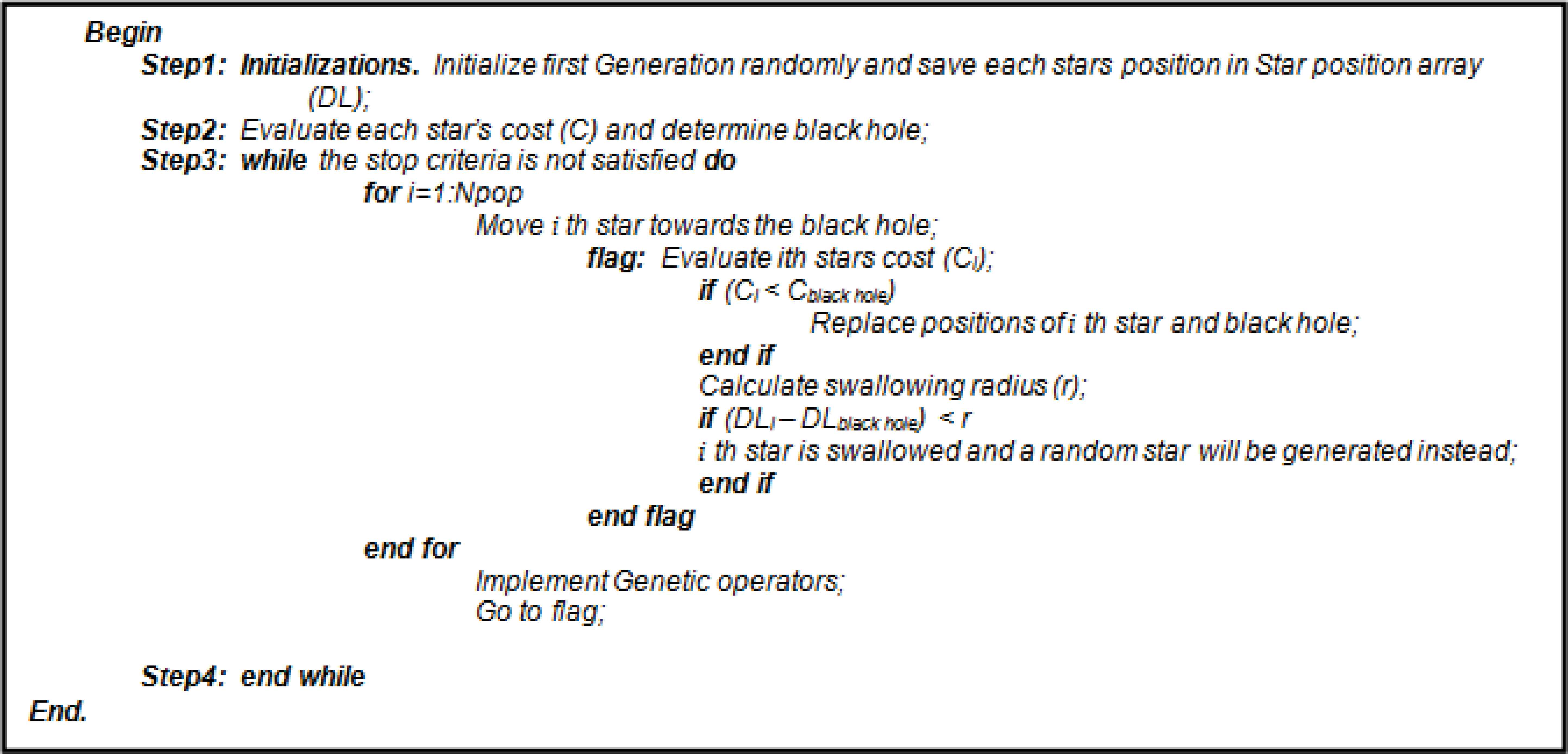
Pseudo-code for Modified Black Hole Algorithm.
4. Experimental Results
In this section, performance of the MBH algorithm is evaluated. The test of reliability, efficiency and validation of optimization algorithms is frequently carried out using a set of standard benchmarks or test functions [27]. The benchmark problems are categorized to low and high dimensional problems. The low dimensional ones are used to test the speed of convergence, however the high dimensional ones are good criterions to evaluate the computing power of an algorithm. In this work, the MBH algorithm has been applied to 20 different benchmark problems including ten low and ten high dimensional problems. Data sets of the problems are shown in Table 1.
| Name | Function | Dimensions | Variables Bound | Global Minimum | ||
|---|---|---|---|---|---|---|
| High-Dimension Benchmark Functions | ||||||
| P1 | Alpine | | 20 | X ∈ [-10,10] | 0 | |
| P2 | Alpine 2 | | 20 | X ∈ [-10,10] | 0 | |
| P3 | csendes | | 20 | X ∈ [-1,1] | 0 | |
| P4 | Deb1 | | 20 | X ∈ [-1,1] | -1 | |
| P5 | Quintic | | 20 | X ∈ [-10,10] | 0 | |
| P6 | Rastrigin | | 20 | X ∈ [-5.12,5.12] | 0 | |
| P7 | Salomon | | 20 | X ∈ [-100,100] | 0 | |
| P8 | Schwefel2.21 | | 20 | X ∈ [-100,100] | 0 | |
| P9 | Schwefel2.26 | | 20 | X ∈ [-500,500] | -418.983 | |
| P10 | Sphere | | 20 | X ∈ [-10,10] | 0 | |
| Low-Dimension Benchmark Functions | ||||||
| P11 | Ackley 2 | | 2 | X ∈ [-32,32] | -200 | |
| P12 | Bartels Conn | | 2 | X ∈ [-500,500] | 1 | |
| P13 | Parsopoulos | | 2 | X ∈ [-5,5] | 0 | |
| P14 | Periodic | | 2 | X ∈ [-10,10] | 0.9 | |
| P15 | Price | | 2 | X ∈ [-500,500] | 0 | |
| P16 | Rotated Ellipse | | 2 | X ∈ [-500,500] | 0 | |
| P17 | Scahffer | | 2 | X ∈ [-500,500] | 0 | |
| P18 | Table 1 | | 2 | X ∈ [-10,10] | 0 | |
| P19 | Ursem 4 | | 2 | X ∈ [-2,2] | 0 | |
| P20 | Hartman 1 | | 3 | X ∈ [0,1] | -3.8628 | |
Benchmark Problems.
The famous peak problem has been selected in order to observe the objective behavior of the MBH algorithm. The contour of the peak problem is shown in Fig. 5 and the corresponding equation is as follows:
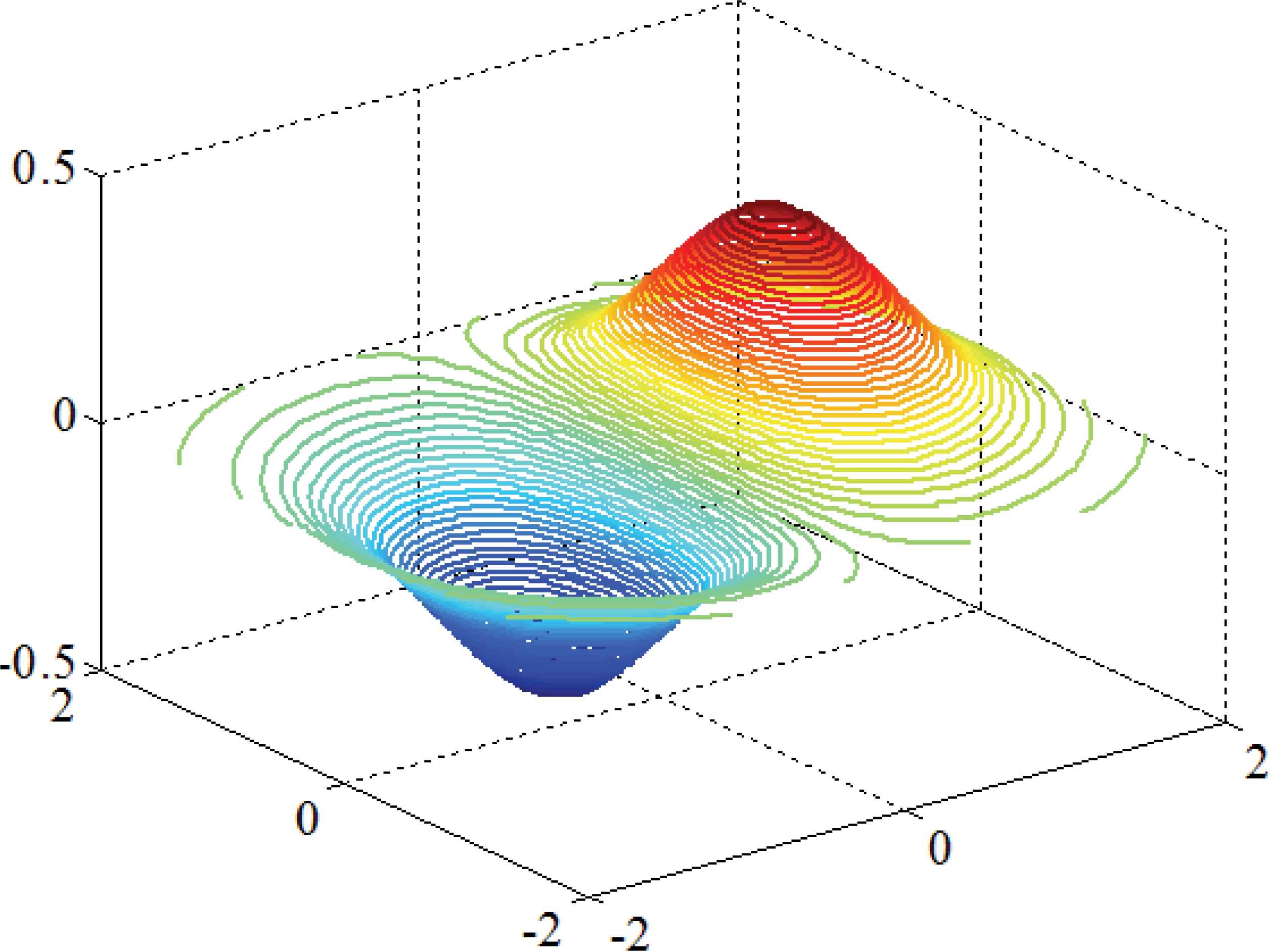
3-D Contour plot of Peak function.
Starting the problem with an initial population of 15 particles. The algorithm behavior from the initial generation to the fourth iteration has been presented in Fig. 6. Initial population of the random generated particles is shown in Fig. 6(a). Location of the particles and the black hole after the first iteration is also presented in Fig. 6(b). As shown, location of the black hole has been changed from (-0.64,0.62) with -0.2876 of cost to the point (-0.83,-0.05) with -0.4141 of cost. In the third iteration, all the particles (stars) have been gathered around the minimum, however, they have not yet reached the global minimum. It should be noted that, in the fourth iteration, some of stars have been distanced from the black hole. It indicates the point in which these stars are too close to the black hole. The black hole starts to omit them and locate these stars in a random point. The algorithm is reached to the global minimum coordinates (-0.708,0.002) with cost of -0.4289 in the fifth iteration of the test. It is obvious that more particles have been omitted in this stage due to their close distance to the black hole. Efficiency and the power of proposed method in terms of detecting the global minimum is expressed in the peak problem.
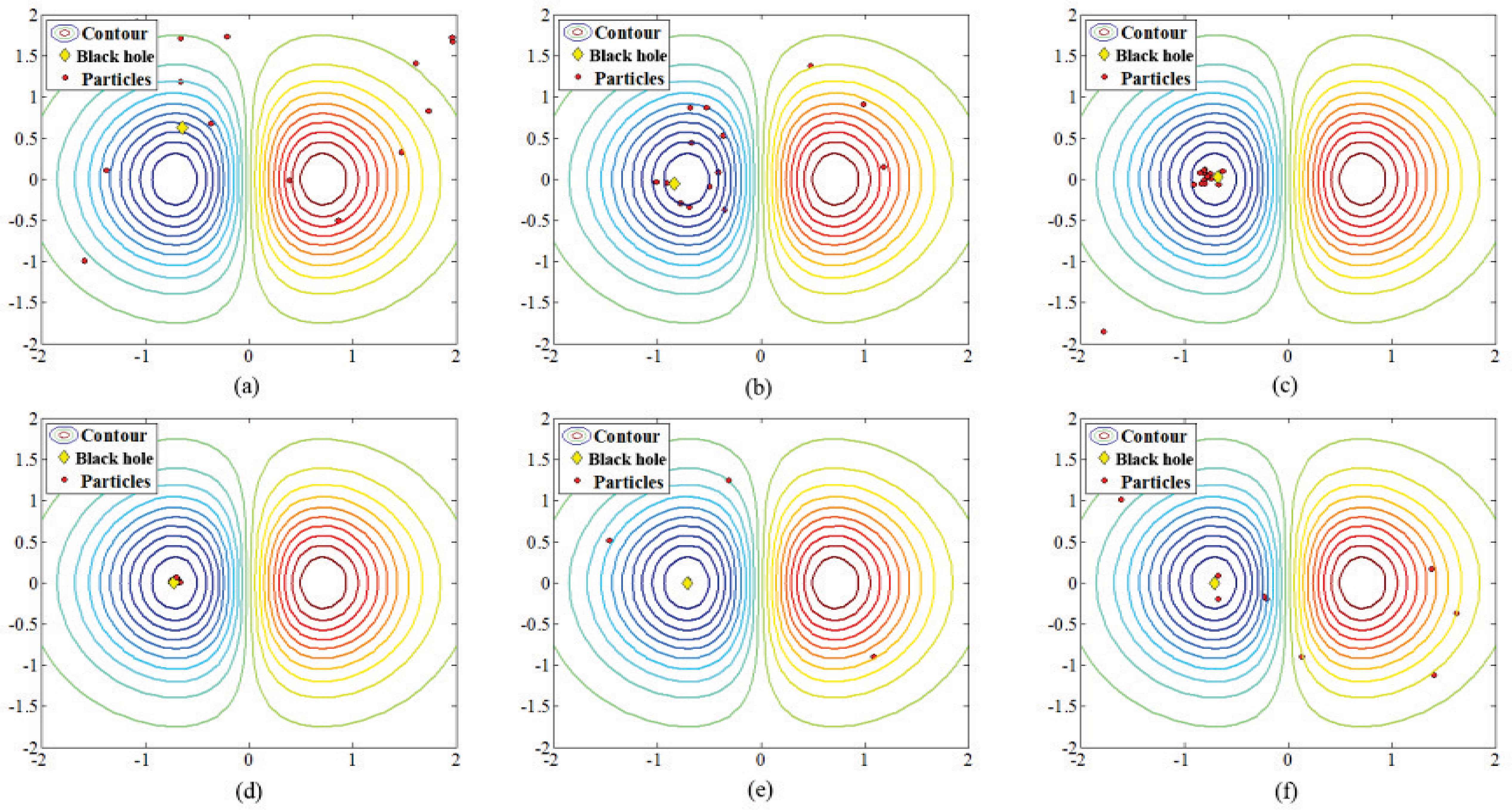
Positions of stars and black hole in (a) Initial generation, (b) 1st iteration, (c) 2nd iteration, (d) 3rd iteration, (e) 4th iteration and (f) 5th iteration.
Now, a two dimensional problem with more than one local minima is considered to test the MBH algorithm performance. A two dimensional problem has been presented in Eq. (15):
There are 18 minimum points in the above-mentioned range, where the point (9.0390, 8.6681) with the cost value of –18.5547 is the global minimum. The three-dimensional overview of the function is presented in Fig. 7.
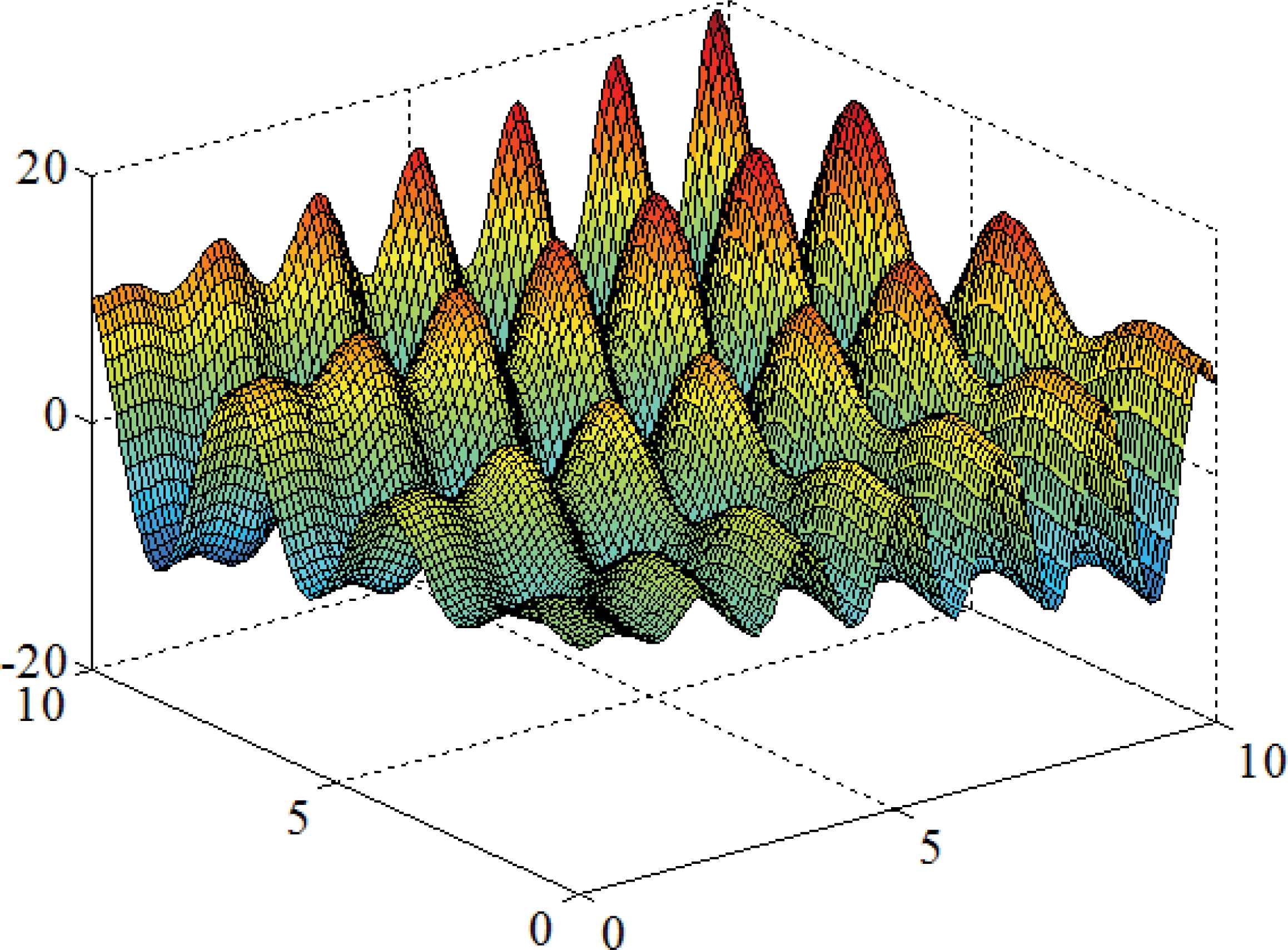
3-D plot of f(x,y) function.
Starting with the initial population of 20, the progress procedure of solution after ten iterations is shown in Fig. 8. In the first iteration, the black hole is placed in local minima. It will gradually find its way near the desired global minimum up to the third iteration. In this stage, the black hole is at (8.9543, 8.5847) with the cost of -17.9116. Its distance is reduced to the global minimum inchmeal, and in the seventh iteration it will arrive to the best point (9.0387, 8.6689). Comparing Fig. 8(e). and Fig. 8(d)., it is clear that the omitting section of the very nigh particles has been done successfully, and the particles contiguous to the black hole have been generated in different coordinates. The diagram of the cost reduction versus iteration is shown in Fig. 9 indicating the point in the fourth iteration. The algorithm has been reduced its distance to the desired minimum and finally, it reaches to its best cost at the seventh iteration.
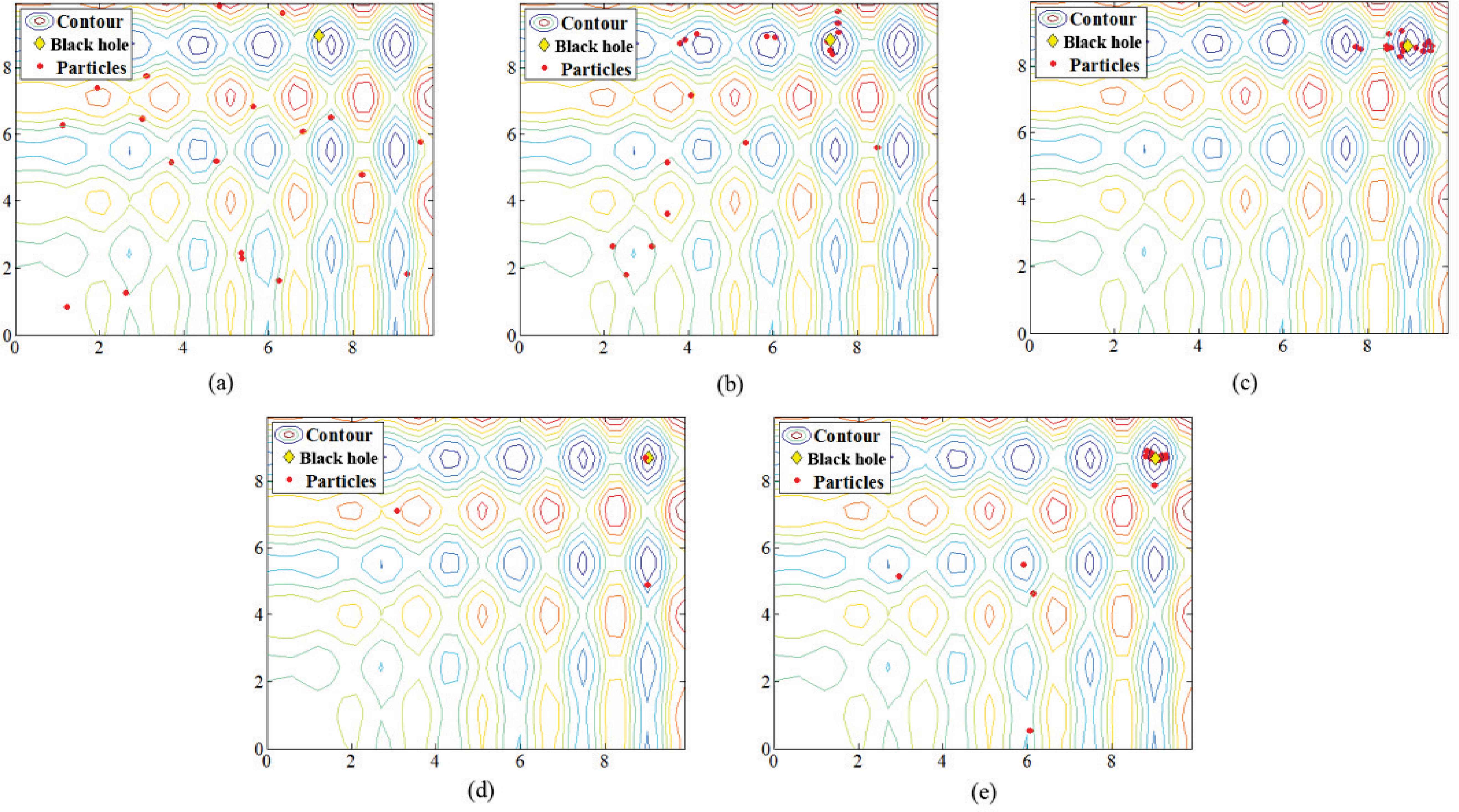
Positions of stars and black hole in (a) Initial generation, (b)1st iteration, (c) 3rd iteration, (d) 5th iteration and (e) 10th iteration.
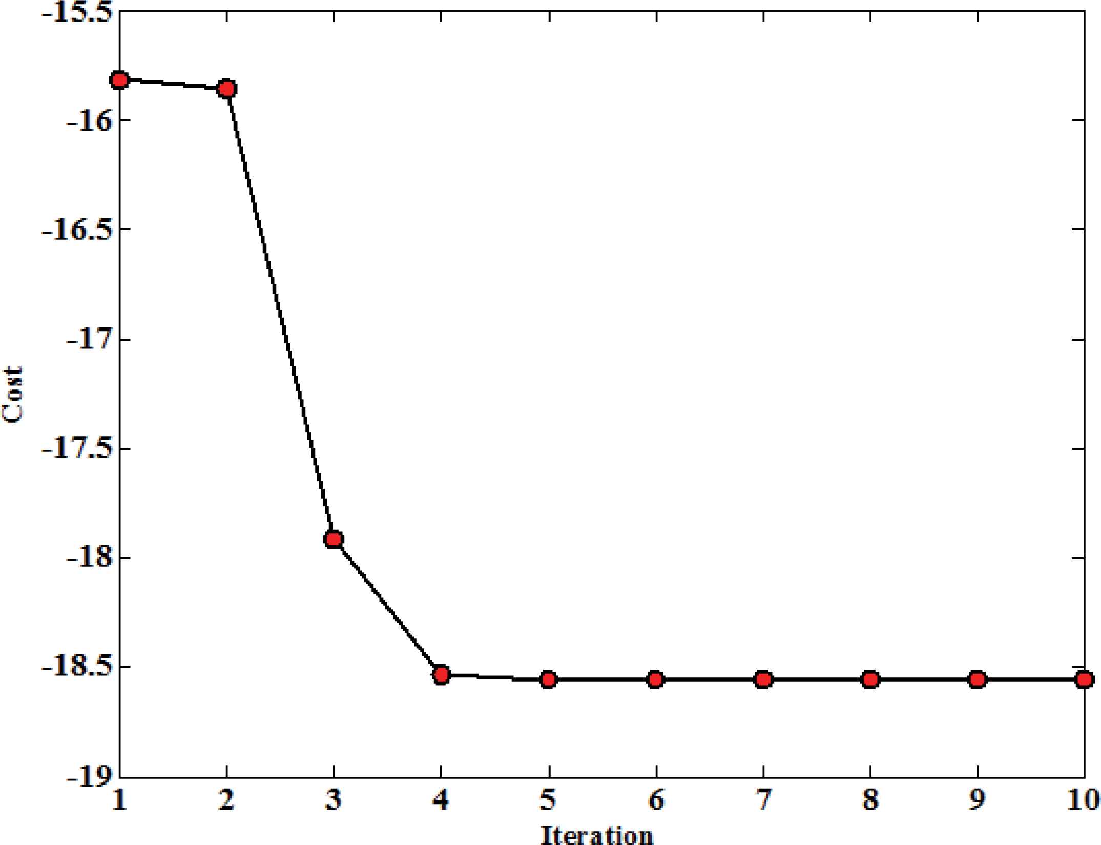
Cost minimization for the problem f(x,y).
As cited earlier in this section, 20 benchmark problems have been tested, and results are obtained. In addition, comparisons with several well-known methods such as PSO, BA, BH, HS [27], and FA, has been presented in order to analyze the performance of the MBH algorithm for different problems. Table 2 shows the parameters of each optimization algorithms. There are various parts with random behavior in these types of algorithms. If such algorithms are applied to different problems once, it may not express exact strengths and weaknesses of experimented method. Therefore, multiplicity of tests should be increased to avoid the lack of cogent gauge and the random behavior effect. For this purpose, procedure of algorithms have been repeated 50 times for each problem to validate the results and obtain clear outcomes. The obtained solutions are presented in Table 3 and Table 4 considering the four factors, namely best, worst, average, and standard deviation. Each algorithm has been initialized with 50 trials. The crossover and mutation operators are utilized and adopted to be 70% and 20%, respectively. The high dimensional problems are presented in Table 3. Since there are many decision variables available in problems P1 to P10, the number of iterations in each run has been set to 250. Therefore, enough time is provided for algorithm to seek the search space completely, however the number of iterations for the low dimensional problems has been considered to be 50. Table 4 shows the resultant of applying various algorithms to low dimensional sets P11 to P20. The modified black hole is marked as the best solutions available against its counterparts, showing the fastest convergence ratio to reach the desirable minimum.
| Algorithm | Parameters |
|---|---|
| PSO | Personal Learning Coefficient (c1) and Global Learning Coefficient (c2): are determined by Constriction Coefficients method [21]. |
| BA | Number of Scout Bees: 30 Number of Selected Sites: 15 Number of Selected Elite Sites: 6 Number of Recruited Bees for Selected Sites: 15 Number of Recruited Bees for Elite Sites: 12 Neighborhood Radius Damp Rate: 0.99 |
| ICA | Number of Empires/Imperialists: 10 Selection Pressure: 1 Assimilation Coefficient: 2 Revolution Probability: 0.1 Revolution Rate: 0.05 Colonies Mean Cost Coefficient: 0.1 |
| FA | Light Absorption Coefficient: 1 Attraction Coefficient Base Value: 2 Mutation Coefficient: 0.2 Mutation Coefficient Damping Ratio: 0.99 |
Algorithms parameters.
| I | ci | aij | pij | |||
|---|---|---|---|---|---|---|
| J=1 | 2 | 3 | J=1 | 2 | ||
| 1 | 1 | 3 | 10 | 30 | 0.3689 | 0.117 |
| 2 | 1.2 | 0.1 | 10 | 35 | 0.4699 | 0.4387 |
| 3 | 3 | 3 | 10 | 30 | 0.1091 | 0.8732 |
| 4 | 3.2 | 0.1 | 10 | 35 | 0.03815 | 0.5743 |
Constants of Hartman1 problem.
| MBH | BH | PSO | BA | ICA | FA | ||
|---|---|---|---|---|---|---|---|
| P11 | -200 | -200 | -199.9999 | -199.9996 | -200 | -199.9995 | Best |
| -199.9999 | -199.9968 | -199.9748 | -199.9879 | -199.9998 | -199.9795 | Worst | |
| -200 | -199.9991 | -199.9937 | -199.9955 | -200 | -199.9921 | Mean | |
| 1.6986e-005 | 0.0007738 | 0.0050905 | 0.0029244 | 3.304e-005 | 0.0048177 | Std. | |
| P12 | 1 | 1 | 1.00005 | 1.0004 | 1 | 1.0003 | Best |
| 1 | 1.033908 | 1.03204 | 1.0312 | 1 | 1.0307 | Worst | |
| 1 | 1.003038 | 1.00819 | 1.0074 | 1 | 1.0082 | Mean | |
| 1.2781e-010 | 0.005630 | 0.007895799 | 0.0061017 | 4.1683e-006 | 0.00693 | Std. | |
| P13 | 7.4988e-033 | 1.536e-018 | 1.2212e-010 | 1.8528e-010 | 8.7737e-020 | 1.2567e-009 | Best |
| 1.148e-023 | 0.013345 | 0.0009338 | 3.6351e-007 | 1.9311e-011 | 4.721e-007 | Worst | |
| 2.7415e-025 | 0.0014562 | 2.5437e-005 | 4.8615e-008 | 6.5184e-013 | 1.1754e-007 | Mean | |
| 1.6321e-024 | 0.0028489 | 0.0001323 | 6.7474e-008 | 2.7816e-012 | 1.0451e-007 | Std. | |
| P14 | 0.9 | 0.9 | 0.9 | 0.9 | 0.9 | 0.9 | Best |
| 1 | 1.0136 | 1.0003 | 1 | 1 | 1 | Worst | |
| 0.9164 | 0.93867 | 0.94773 | 0.92014 | 0.93921 | 0.992 | Mean | |
| 0.036639 | 0.049791 | 0.050002 | 0.04034 | 0.048462 | 0.037405 | Std. | |
| P15 | 0 | 1.9824e-021 | 3.4774e-006 | 2.6024e-006 | 9.1726e-015 | 4.5209e-005 | Best |
| 1.9474e-021 | 6.4145e-007 | 0.019067 | 0.00056819 | 1.0025e-005 | 0.0042154 | Worst | |
| 3.8956e-023 | 2.5181e-008 | 0.0031429 | 0.00012437 | 2.1503e-007 | 0.0010889 | Mean | |
| 2.7541e-022 | 9.5795e-008 | 0.0047193 | 0.00013662 | 1.4173e-006 | 0.00093021 | Std. | |
| P16 | 1.7809e-036 | 4.1122e-019 | 9.8908e-006 | 0.00010058 | 6.4237e-013 | 9.0579e-005 | Best |
| 1.1952e-023 | 0.027406 | 0.047892 | 0.041529 | 0.00032499 | 1.9692 | Worst | |
| 1.0299e-024 | 0.0014927 | 0.0077412 | 0.01229 | 1.2746e-005 | 0.051312 | Mean | |
| 2.6402e-024 | 0.0053704 | 0.010168 | 0.011859 | 4.8577e-005 | 0.27717 | Std. | |
| P17 | 0 | 0 | 1.1102e-016 | 2.8522e-013 | 0 | 2.3981e-014 | Best |
| 0 | 2.3804e-007 | 5.3775e-009 | 1.4302e-008 | 0.0092577 | 9.9654e-009 | Worst | |
| 0 | 4.7607e-009 | 1.5558e-010 | 7.388e-010 | 0.0003093 | 1.3847e-009 | Mean | |
| 0 | 3.3664e-008 | 7.7712e-010 | 2.2204e-009 | 0.0015614 | 2.6762e-009 | Std. | |
| P18 | 4.7945e-033 | 3.1004e-025 | 3.8976e-011 | 3.2972e-011 | 1.1365e-020 | 4.3332e-011 | Best |
| 6.9868e-024 | 2.6222e-011 | 0.00017361 | 3.0583e-007 | 2.9605e-013 | 3.2899e-007 | Worst | |
| 1.511e-025 | 5.4595e-013 | 2.1481e-005 | 3.4525e-008 | 9.1173e-015 | 7.2566e-008 | Mean | |
| 9.8815e-025 | 3.7084e-012 | 3.8908e-005 | 5.1877e-008 | 4.2239e-014 | 9 .0057e-008 | Std. | |
| P19 | 0 | 0 | 1.452e-010 | 5.7192e-011 | 0 | 0 | Best |
| 1.8171e-013 | 1.5377e-007 | 2.1603e-005 | 2.6426e-008 | 3.2401e-013 | 8.1493e-008 | Worst | |
| 6.5718e-015 | 5.7845e-009 | 1.5408e-006 | 2.6765e-009 | 1.0084e-014 | 2.7983e-009 | Mean | |
| 2.917e-014 | 2.8146e-008 | 4.4988e-006 | 5.3208e-009 | 4.7946e-014 | 1.1505e-008 | Std. | |
| P20 | -3.8628 | -3.8626 | -3.8628 | -3.8628 | -3.8628 | -3.8628 | Best |
| -3.8628 | -3.8259 | -3.8549 | -3.8628 | -3.8628 | -3.8628 | Worst | |
| -3.8628 | -3.85 | -3.8626 | -3.8628 | -3.8628 | -3.8628 | Mean | |
| 1.2449e-008 | 0.0077845 | 0.0011145 | 1.2817e-007 | 5.9477e-008 | 4.9129e-007 | Std. | |
Best, worst, mean and the standard deviation of available solution in MBH and BH, PSO, BA, ICA, FA for low-dimension benchmark problems.
In order to improve the comparison procedure, the cost versus iteration diagram of PSO, MBH, and BA for a random test has been plotted in Fig. 10. The Alpine problem (P1) is studied in Fig. 10(a). The MBH algorithm converges to the desired global minimum with the best cost in the 49th iteration, while the two other methods do not reach the minimum after 250th iteration. Fig. 10(b) presents solutions of the discussed algorithms to a high dimensional problem called as Csendes (P3). Although all the three algorithms start the process almost alike, nearly with the same cost, MBH presents the best speed of convergence and better performance compared with the two other algorithms after 250 iteration. The cost minimization plot of the three aforementioned algorithms for the problems called as Ackley 2 (P11) and Schaffer (P17) is shown in Fig. 10(c)-(d). As it is clear in Fig. 10(c), although the initial cost of MBH is much more than the others, but the best global optimum is obtained in the fifth iteration whereas the iteration number for the best solution is 11 for BA and 25 for PSO. Another example is shown in Fig. 10(d) where the seeking process is started with approximately the same initial cost. MBH has reached the best optimum in the eleventh iteration, while BA and PSO are incapable of reaching the optimum even after 50 times of iterations.
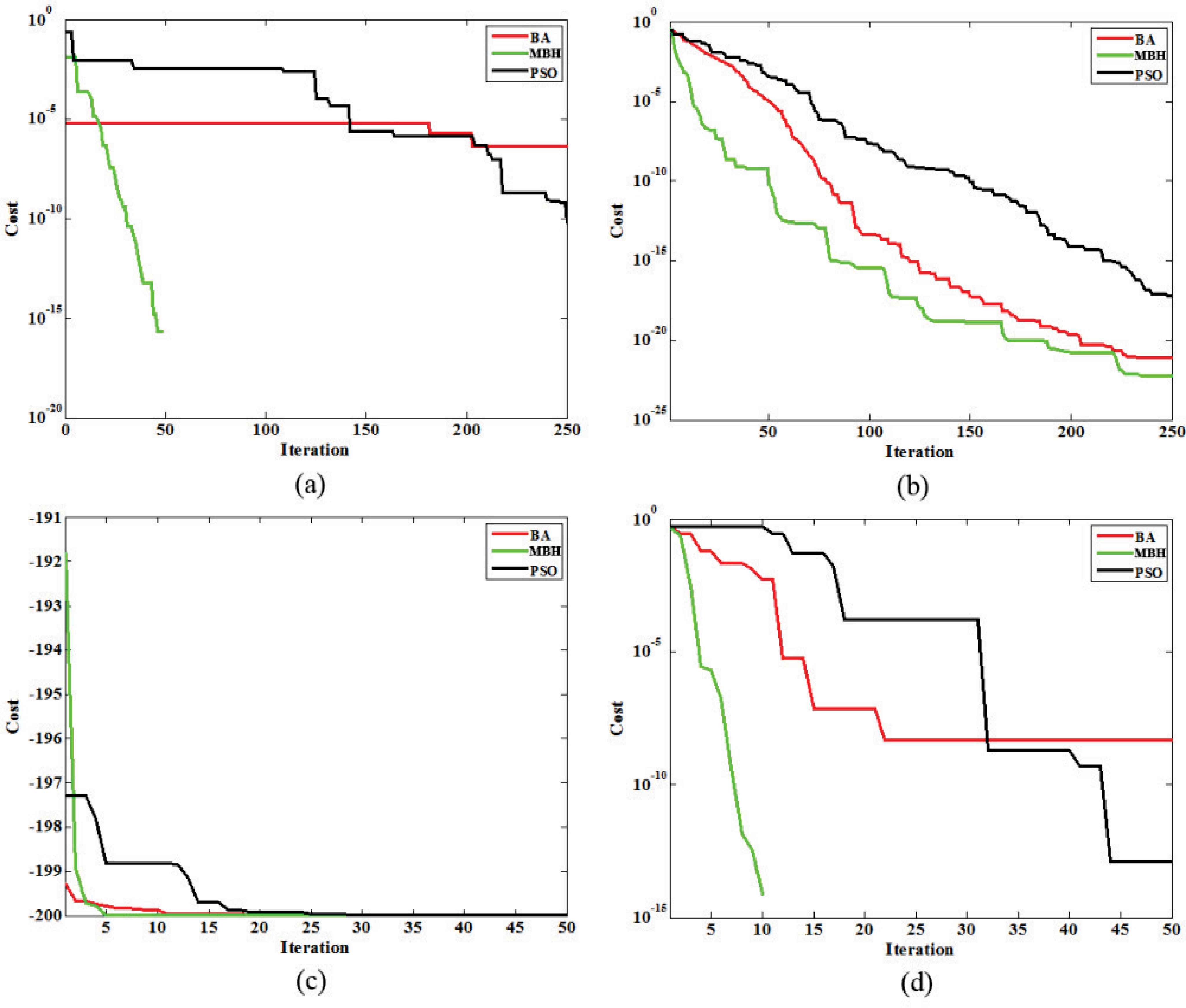
Comparison of the cost convergence of BA, MBH and PSO for (a) P1, (b) P3, (c) P11 and (d) P17 problems.
Finally, the worst, mean, and best run of the cost minimization plot of MBH algorithm for six different problems are presented in Fig. 11. As shown in Fig. 11(a) and Fig. 11(f), when the MBH algorithm reach to the 100% of accuracy i.e. zero for the cited problems, the figures are corrupted. The reason is that the logarithmic plots are incapable of representing zero.
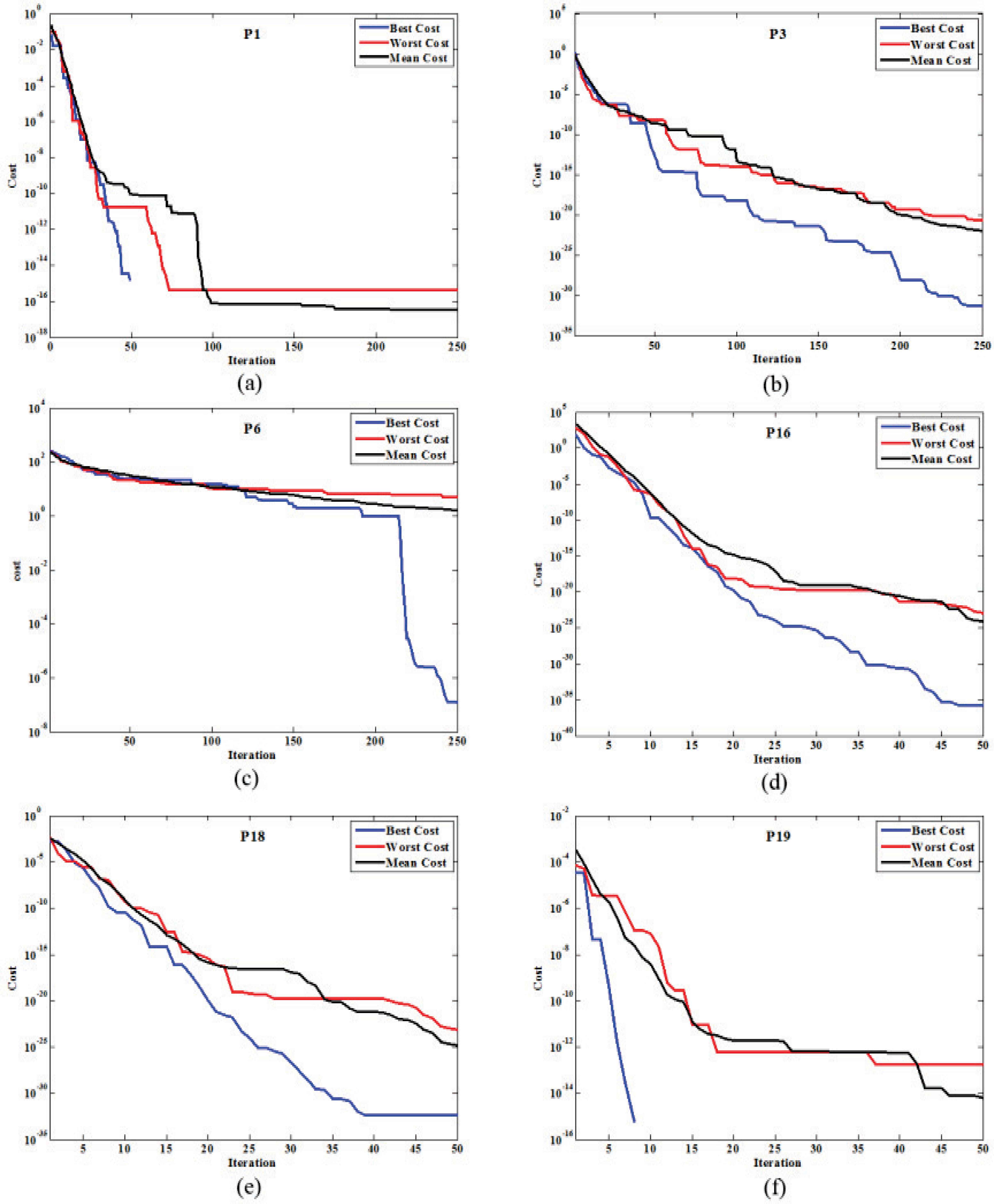
Cost minimization of Modified Black Hole algorithm in best, worst and mean test in 50 tests for (a) P1, (b) P3, (c) P6, (d) P16, (e) P18 and (f) P19 problems, where the exact solutions have been obtained in figures (a) and (f) in the best run.
5. Conclusion
In this paper, the modified Black Hole algorithm has been proposed for solving optimization problems. A new approach is employed to overcome the probable drawbacks caused by the trapping effect, where trapping is suppressed and particles close to the black hole are swallowed with a new swallowing range if they exceed the minimum distance to the black hole. Afterwards, a new particle is generated in the search space randomly to avoid probable disturbances of trapping effect. The proposed algorithm has been applied to 20 different benchmark problems on 50 tests, and the results are compared with the standard Black Hole algorithm and its other counterparts. It is clear that the proposed method presents various remarkable superiorities than the other well-known optimization algorithms such as BH, PSO, BA, ICA, and FA. Also, the MBH outperforms the others in 17 of 20 problems. It is more prominent that the exact solutions (100% accuracy in the best runs) are obtained for 10 problems, showing the power and highly accurate performance of the Modified Black Hole algorithm.
| MBH | BH | PSO | BA | ICA | FA | ||
|---|---|---|---|---|---|---|---|
| P11 | -200 | -200 | -199.9999 | -199.9996 | -200 | -199.9995 | Best |
| -199.9999 | -199.9968 | -199.9748 | -199.9879 | -199.9998 | -199.9795 | Worst | |
| -200 | -199.9991 | -199.9937 | -199.9955 | -200 | -199.9921 | Mean | |
| 1.6986e-005 | 0.0007738 | 0.0050905 | 0.0029244 | 3.304e-005 | 0.0048177 | Std. | |
| P12 | 1 | 1 | 1.00005 | 1.0004 | 1 | 1.0003 | Best |
| 1 | 1.033908 | 1.03204 | 1.0312 | 1 | 1.0307 | Worst | |
| 1 | 1.003038 | 1.00819 | 1.0074 | 1 | 1.0082 | Mean | |
| 1.2781e-010 | 0.005630 | 0.007895799 | 0.0061017 | 4.1683e-006 | 0.00693 | Std. | |
| P13 | 7.4988e-033 | 1.536e-018 | 1.2212e-010 | 1.8528e-010 | 8.7737e-020 | 1.2567e-009 | Best |
| 1.148e-023 | 0.013345 | 0.0009338 | 3.6351e-007 | 1.9311e-011 | 4.721e-007 | Worst | |
| 2.7415e-025 | 0.0014562 | 2.5437e-005 | 4.8615e-008 | 6.5184e-013 | 1.1754e-007 | Mean | |
| 1.6321e-024 | 0.0028489 | 0.0001323 | 6.7474e-008 | 2.7816e-012 | 1.0451e-007 | Std. | |
| P14 | 0.9 | 0.9 | 0.9 | 0.9 | 0.9 | 0.9 | Best |
| 1 | 1.0136 | 1.0003 | 1 | 1 | 1 | Worst | |
| 0.9164 | 0.93867 | 0.94773 | 0.92014 | 0.93921 | 0.992 | Mean | |
| 0.036639 | 0.049791 | 0.050002 | 0.04034 | 0.048462 | 0.037405 | Std. | |
| P15 | 0 | 1.9824e-021 | 3.4774e-006 | 2.6024e-006 | 9.1726e-015 | 4.5209e-005 | Best |
| 1.9474e-021 | 6.4145e-007 | 0.019067 | 0.00056819 | 1.0025e-005 | 0.0042154 | Worst | |
| 3.8956e-023 | 2.5181e-008 | 0.0031429 | 0.00012437 | 2.1503e-007 | 0.0010889 | Mean | |
| 2.7541e-022 | 9.5795e-008 | 0.0047193 | 0.00013662 | 1.4173e-006 | 0.00093021 | Std. | |
| P16 | 1.7809e-036 | 4.1122e-019 | 9.8908e-006 | 0.00010058 | 6.4237e-013 | 9.0579e-005 | Best |
| 1.1952e-023 | 0.027406 | 0.047892 | 0.041529 | 0.00032499 | 1.9692 | Worst | |
| 1.0299e-024 | 0.0014927 | 0.0077412 | 0.01229 | 1.2746e-005 | 0.051312 | Mean | |
| 2.6402e-024 | 0.0053704 | 0.010168 | 0.011859 | 4.8577e-005 | 0.27717 | Std. | |
| P17 | 0 | 0 | 1.1102e-016 | 2.8522e-013 | 0 | 2.3981e-014 | Best |
| 0 | 2.3804e-007 | 5.3775e-009 | 1.4302e-008 | 0.0092577 | 9.9654e-009 | Worst | |
| 0 | 4.7607e-009 | 1.5558e-010 | 7.388e-010 | 0.0003093 | 1.3847e-009 | Mean | |
| 0 | 3.3664e-008 | 7.7712e-010 | 2.2204e-009 | 0.0015614 | 2.6762e-009 | Std. | |
| P18 | 4.7945e-033 | 3.1004e-025 | 3.8976e-011 | 3.2972e-011 | 1.1365e-020 | 4.3332e-011 | Best |
| 6.9868e-024 | 2.6222e-011 | 0.00017361 | 3.0583e-007 | 2.9605e-013 | 3.2899e-007 | Worst | |
| 1.511e-025 | 5.4595e-013 | 2.1481e-005 | 3.4525e-008 | 9.1173e-015 | 7.2566e-008 | Mean | |
| 9.8815e-025 | 3.7084e-012 | 3.8908e-005 | 5.1877e-008 | 4.2239e-014 | 9 .0057e-008 | Std. | |
| P19 | 0 | 0 | 1.452e-010 | 5.7192e-011 | 0 | 0 | Best |
| 1.8171e-013 | 1.5377e-007 | 2.1603e-005 | 2.6426e-008 | 3.2401e-013 | 8.1493e-008 | Worst | |
| 6.5718e-015 | 5.7845e-009 | 1.5408e-006 | 2.6765e-009 | 1.0084e-014 | 2.7983e-009 | Mean | |
| 2.917e-014 | 2.8146e-008 | 4.4988e-006 | 5.3208e-009 | 4.7946e-014 | 1.1505e-008 | Std. | |
| P20 | -3.8628 | -3.8626 | -3.8628 | -3.8628 | -3.8628 | -3.8628 | Best |
| -3.8628 | -3.8259 | -3.8549 | -3.8628 | -3.8628 | -3.8628 | Worst | |
| -3.8628 | -3.85 | -3.8626 | -3.8628 | -3.8628 | -3.8628 | Mean | |
| 1.2449e-008 | 0.0077845 | 0.0011145 | 1.2817e-007 | 5.9477e-008 | 4.9129e-007 | Std. | |
Best, worst, mean and the standard deviation of available solution in MBH and BH, PSO, BA, ICA, FA for low-dimension benchmark problems.
References
Cite this article
TY  - JOUR
AU  - Saber Yaghoobi
AU  - Hamed Mojallali
PY  - 2016
DA  - 2016/08/01
TI  - Modified Black Hole Algorithm with Genetic Operators
JO  - International Journal of Computational Intelligence Systems
SP  - 652
EP  - 665
VL  - 9
IS  - 4
SN  - 1875-6883
UR  - https://doi.org/10.1080/18756891.2016.1204114
DO  - 10.1080/18756891.2016.1204114
ID  - Yaghoobi2016
ER  -