
A hybrid gene expression programming algorithm based on orthogonal design
- DOI
- 10.1080/18756891.2016.1204124How to use a DOI?
- Keywords
- Evolutionary computation; Gene expression programming; Orthogonal design; Evolutionary stable strategy
- Abstract
The last decade has witnessed a great interest on the application of evolutionary algorithms, such as genetic algorithm (GA), particle swarm optimization (PSO) and gene expression programming (GEP), for optimization problems. This paper presents a hybrid algorithm by combining the GEP algorithm and the orthogonal design method. A multiple-parent crossover operator is introduced for the chromosome reproduction using the orthogonal design method. In addition, an evolutionary stable strategy is also employed to maintain the population diversity during the evolution. The efficiency of the proposed algorithm is evaluated using three benchmark problems. The results demonstrate that the proposed hybrid algorithm has a better generalization ability compared to conventional algorithms.
- Copyright
- © 2016. the authors. Co-published by Atlantis Press and Taylor & Francis
- Open Access
- This is an open access article under the CC BY-NC license (http://creativecommons.org/licences/by-nc/4.0/).
1. Introduction
In recent years, evolutionary algorithms have received a great deal of attention for its wide applications 29,10,28. In particular, the gene expression programming (GEP) is acknowledged as a powerful and problem-independent algorithm for multivariate optimization 11,12,31,21. Compared to conventional evolutionary algorithms, it has the similar flowchart which begins with an initial population of chromosomes or individuals. All chromosomes are evaluated based on a predefined fitness function and this population then reproduces the next generation via one or more genetic operators. Finally the best individual with highest fitness is selected as the final output. Numerical experiments demonstrate that GEP has a significantly better performance compared to genetic algorithm (GA) 27,30 and genetic programming (GP) 1,17, and surpasses those conventional methods by more than two orders of magnitude 10,11,12. However, GEP has also been shown to have certain disadvantages, such as slow convergence and low solution accuracy, particularly for problems with a high-dimensional and large space 4,6,24.
The orthogonal design (OD) is an efficient method for experimental design and analysis 7,9,19. It scatters the test samples uniformly over the feasible space with less computational cost and allows the statistical testing to be conducted over only a few combinations of factors rather than all the possible combinations in an experiment. The OD-based methods have been applied to many areas such as computer experiments 33, electromagnetic devices design 18, and pumping system 14, to improve the capability of problem solving.
Orthogonal design is also combined with many evolutionary algorithm (such as genetic algorithm (GA), particle swarm optimization (PSO), and simulated annealing (SA)) as a local optimization technique. For instance, the orthogonal design method was used in a GA-based algorithm to improve the crossover while reproducing the population in 19. As a result, the offspring were scattered uniformly over the solution space. Similarly, a crossover operator formed by the orthogonal array and the factor analysis was presented in 20. Bayraktar et al. proposed a novel PSO using orthogonal design 3. Instead of the generating-and-updating model in the standard PSO, the orthogonal design method was applied to determine the possible movements of the candidate particles. The OD-based method was employed for initial population generation instead of random sampling in 15. The results showed that the orthogonal design is capable of finding optimal solutions with orthogonal sampling. A hybrid algorithm using SA and orthogonal design was proposed in 2. The orthogonal table and a fractional factorial analysis was used to extract the best combination of decision vectors for simulated annealing, thereby improving the solution accuracy.
Inspired by the preliminary research, we propose a hybrid GEP algorithm based on the OD method, which is named the orthogonal gene expression programming algorithm (OGEP). In OGEP, each bit character from the individual or chromosome is regarded as a factor and the goal of finding the best chromosome is equivalent to searching for the best combination of all factors. The OD-based crossover is then proposed to optimize the factor search. We further employ the evolutionary stable strategy (ESS) 8,26 to maintain the population diversity by controlling the number of the best chromosomes. Compared to the conventional GEP algorithm, the proposed OGEP algorithm has the following properties.
- •
The OD-based crossover involves more than two parent chromosomes for reproduction compared to traditional GEP algorithm.
- •
The OD-based crossover is directly applied on selected chromosomes, which searches for the best combination of genes among candidates.
- •
The number of chromosomes with high fitness is controlled within a certain amount to allow the survival of low-fitness chromosomes, thereby enhancing the population diversity.
The remainder of paper is organized as follows. In Section 2, we briefly review the concept of the conventional GEP algorithm and the orthogonal design method. We then introduce the OGEP algorithm based on the multiple-parent crossover and evolutionary stable strategy in Section 3. Finally, we compare the OGEP algorithm through experiments in Section 4 and conclude our work in Section 5.
2. The GEP algorithm and the orthogonal design method
This section provides some background principles and preliminaries for the standard GEP algorithm and orthogonal design method.
2.1. GEP algorithm
GEP is proposed as a genotype/phenotype genetic algorithm 10,31,21. The procedure of the GEP algorithm shares many common steps with other evolutionary algorithms. For instance, it starts with an initial population which will be evolved until the termination criterion is reached. Then the best chromosome is selected as the final output according to the predefined fitness function.
The fundamental difference between the GEP and other evolutionary algorithms (such as GA or GP) comes from the representation of the chromosomes. In GEP a single chromosome may consist of more than one genes, while each gene is composed of a head and a tail. The head includes the function symbols (such as the plus, minus operation, etc.) and terminal symbols (such as variables or constants); while the tail only contains the terminal symbols. During the evolutionary process, the chromosome is represented as a linear string in GEP. Then, the conventional crossover or mutation operator in GA or GP is applicable in GEP as well. Nevertheless, when it comes to evaluating the fitness, the chromosome will be encoded into a non-linear expression tree (ET) model, which is also known as the K-expressions. Figure 1 gives an example of how a chromosome being encoded into the ET model in GEP.
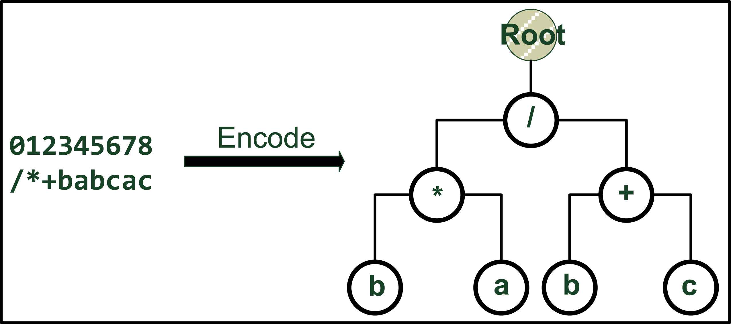
The encoded ET model (right) for a linear chromosome (left). The example chromosome consists of one gene, which is represented by a 9-bit character.
The starting position from K-expressions corresponds to the root of ET, while the branches are replaced with items from the function or terminal set. The K-expressions structure is completely different from either prefix or postfix expression used in GA or GP, which allows for wider degrees of complexity. Because of the K-expressions, the research shows that conventional generic operator, such as the mutation, has a much more profound effect on chromosomes than other algorithms: it usually drastically reshapes the ET structure in GEP, thereby changing the individual fitness. For instance, Figure 2 shows how the mutation operator changes a ET model significantly. The 3rd-bit character in the chromosome from Figure 1 is changed from “b” to “-”. As a result, the encoded ET model is modified considerably and two more branches are generated on the bottom right. That is, conventional genetic operators have a more significant effect on the GEP based chromosomes. The representation and encoding strategy in GEP makes the chromosomes supporting more genome modification 10,11.
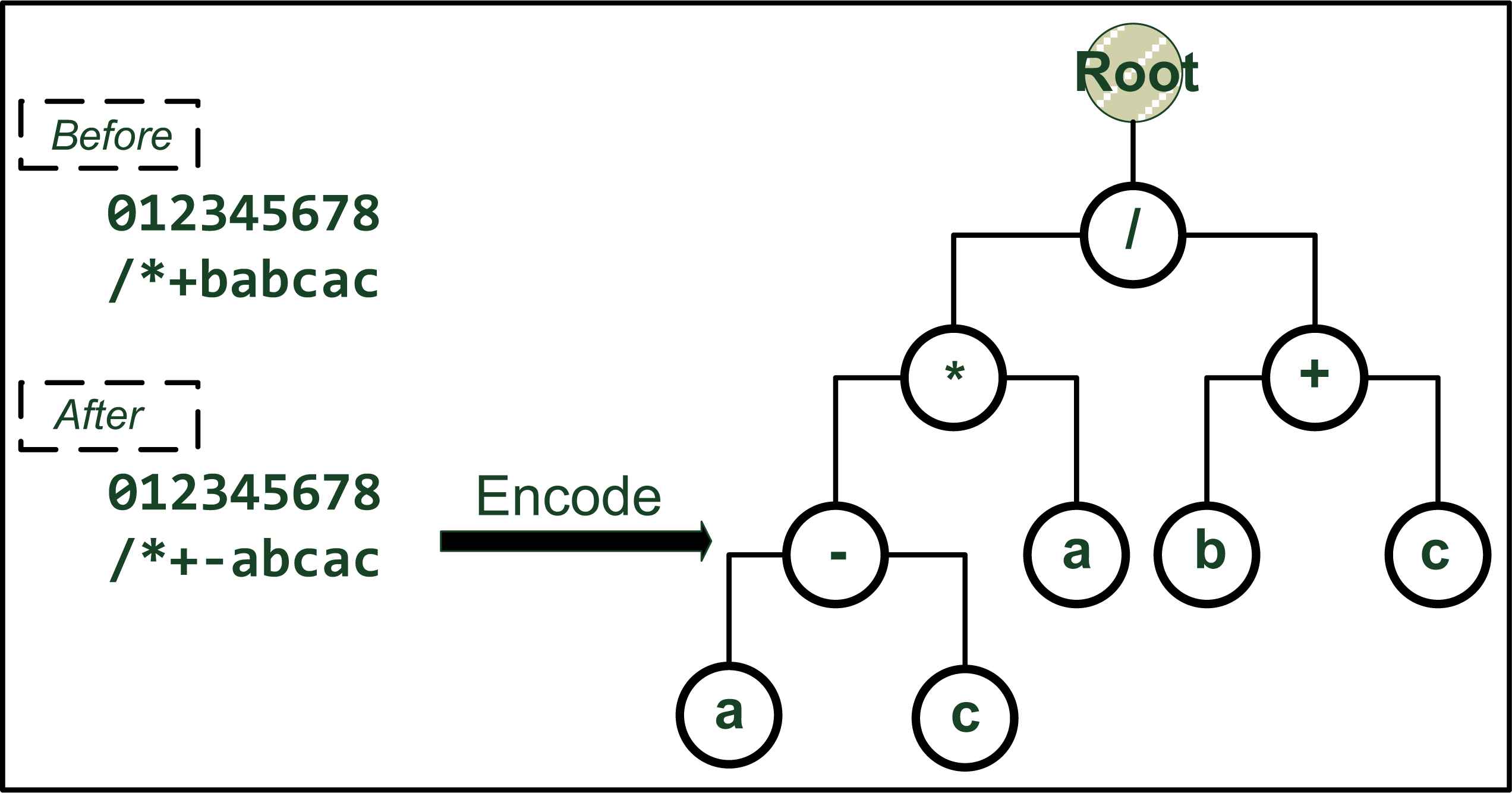
The ET structure before and after the mutation, which indicates the profound effect from the K-expressions in GEP.
Many experiments have been conducted to analyse the performance of the GEP. We refer the reader to 31,24,4 for a more detailed discussion on GEP and its wide applications. The simulation results show that the GEP algorithm achieves a much better performance, which surpasses GA and GP by more than two orders of magnitude.
2.2. Orthogonal design
Orthogonal design has been developed as a mathematical tool to study multiple-factor and multiple-level problems 9,19,7. Consider an experiment that involves some factors and each of which have several possible values called levels. Suppose that there are P factors, each factor has Q levels. The number of combinations of levels of those factors is QP; and for larger P and Q it is not practical to evaluate all combinations.
Based on OD, an orthogonal array AM(QP) (where A stands for the orthogonal array, M is the row number, P is the column number, and Q indicates that one column has Q different values) is computed, where each row represents a combination to be evaluated in an experiment. The orthogonal array has the following key advantages.
- 1.
From the orthogonal array, only a small set of M samples will be selected from all possible QP combinations, commonly M << QP;
- 2.
Each column represents a factor. If some columns are deleted from the array, it means a smaller number of factors are considered;
- 3.
The columns of the array are orthogonal to each other. The selected subset is scattered uniformly over the search space to ensure its diversity.
An efficient method is proposed in 19 to generate an orthogonal array A where M = Q × Q and P = Q+1. The procedures of this method are shown in Algorithm 1.
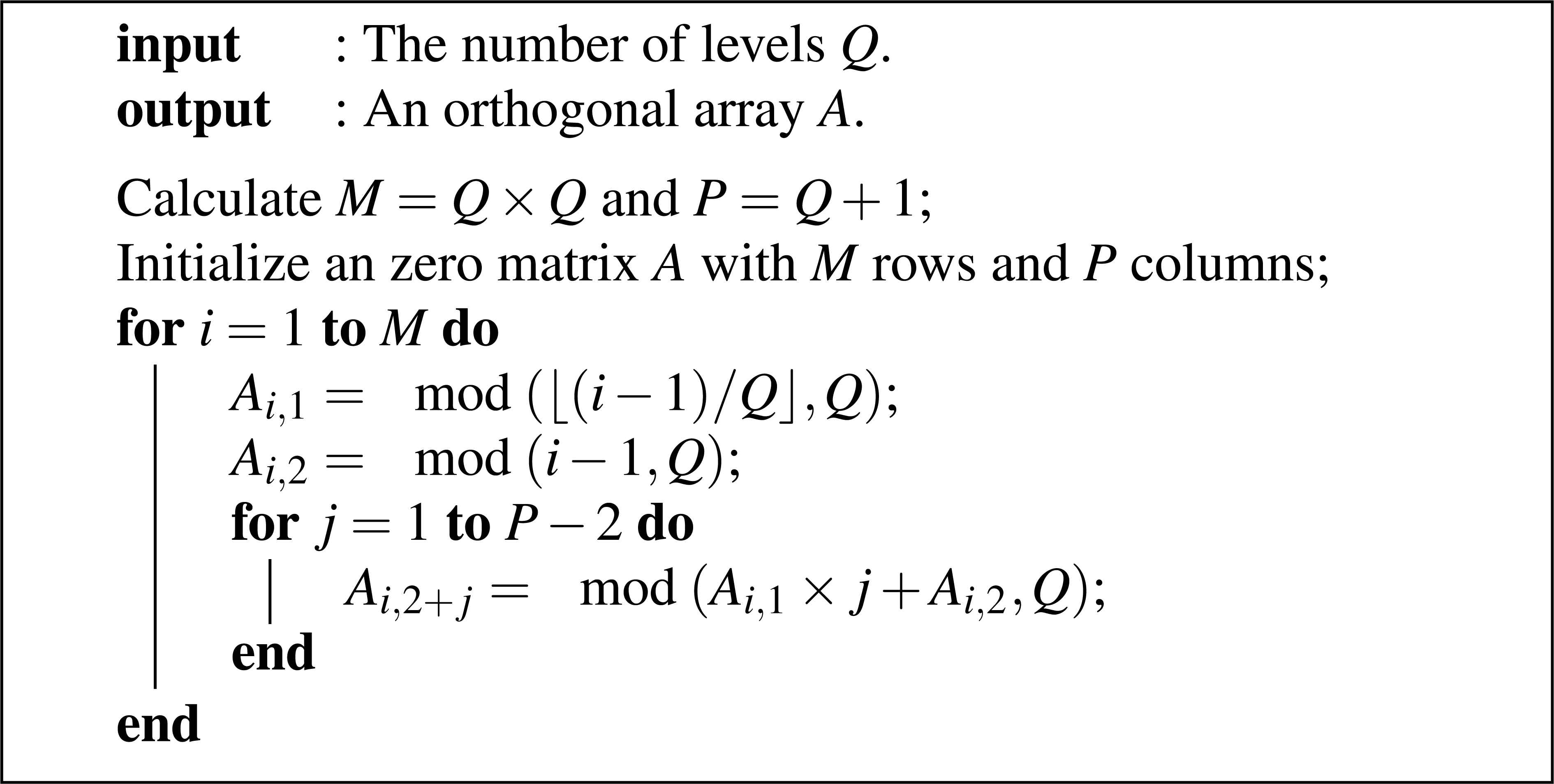
Procedure of the orthogonal array A generation. The mod(*) function represents the modulo operation and ⌊(*)⌋ is the floor function.
Based on the orthogonal design method, the OGEP algorithm is proposed in the next section. The main feature is that the OGEP algorithm employs the OD method for population reproduction, that is capable of generating the offspring uniformly over the search space.
3. The orthogonal gene expression programming (OGEP) algorithm
In this section, we describe the OGEP algorithm which combines the conventional GEP and the orthogonal design method. First the representation of the chromosomes in GEP is shown. Then we introduce the multiple-parent crossover operator, and employ the evolutionary stable strategy for population evolution. We finally summary the main procedure of the proposed OGEP algorithm.
3.1. Chromosome representation
In the GEP algorithm, each solution to the optimization problem is represented as a chromosome. Furthermore, one chromosome is composed of more than one genes. A mathematical or boolean function with more than two arguments (such as the plus operation) can then be used as the linking function, which is used to combine individual genes together into one chromosome. The number of genes in one chromosome and the type of linking function can be a priori chosen for specific problems. Without loss of generality, in this paper we mainly consider the single-gene chromosome, which can be extended to the multiple-gene case by adding any linking function.
One single gene consists of two parts: a head and a tail. Again, the head consists of either function or terminal symbols while the tail only contains the terminals. Let h and t be the length of the head and tail, respectively. Then a chromosome in GEP is encoded in the form of
The length condition in Eq. (2) guarantees that each chromosome in the GEP algorithm can be transferred to a valid expression tree. For simplicity, we further assume that only the operations with two arguments are considered in the head. Thus, we have k = 2 and L = 2 × h + 1.
3.2. Multiple-parent crossover operator
The conventional GEP algorithm reproduces the chromosome using three crossover operators: one-point recombination crossover, two-point recombination crossover, and gene recombination crossover. Nevertheless, the majority crossovers are based on two selected patents. Since only two chromosomes are involved in reproduction, there will be a limited combination of gene structures 20,15,3. To increase the diversity for offspring, the multiple-parent crossover is employed, which employs more than two chromosomes at one time. Then more combinations of gene structures will be expected from different parents. As a result, the multiple-parent crossover operator is able to explore more effectively the search space than the classical two-parent based crossover.
Suppose that we randomly select m chromosomes for the crossover. Note that each chromosome is represented as an L-length string, in which each character from the string can be regarded as a factor. Therefore, with m chromosomes, there are mL combinations in total. To completely explore all the possible combinations is not practical, particularly for a large value of m or L. Meanwhile, the full exploration is also very time-consuming.
To address this problem, the OD method is then employed to select the representative cases from all the possible mL combinations. The procedure of OD-based crossover is detailed in Algorithm 2.
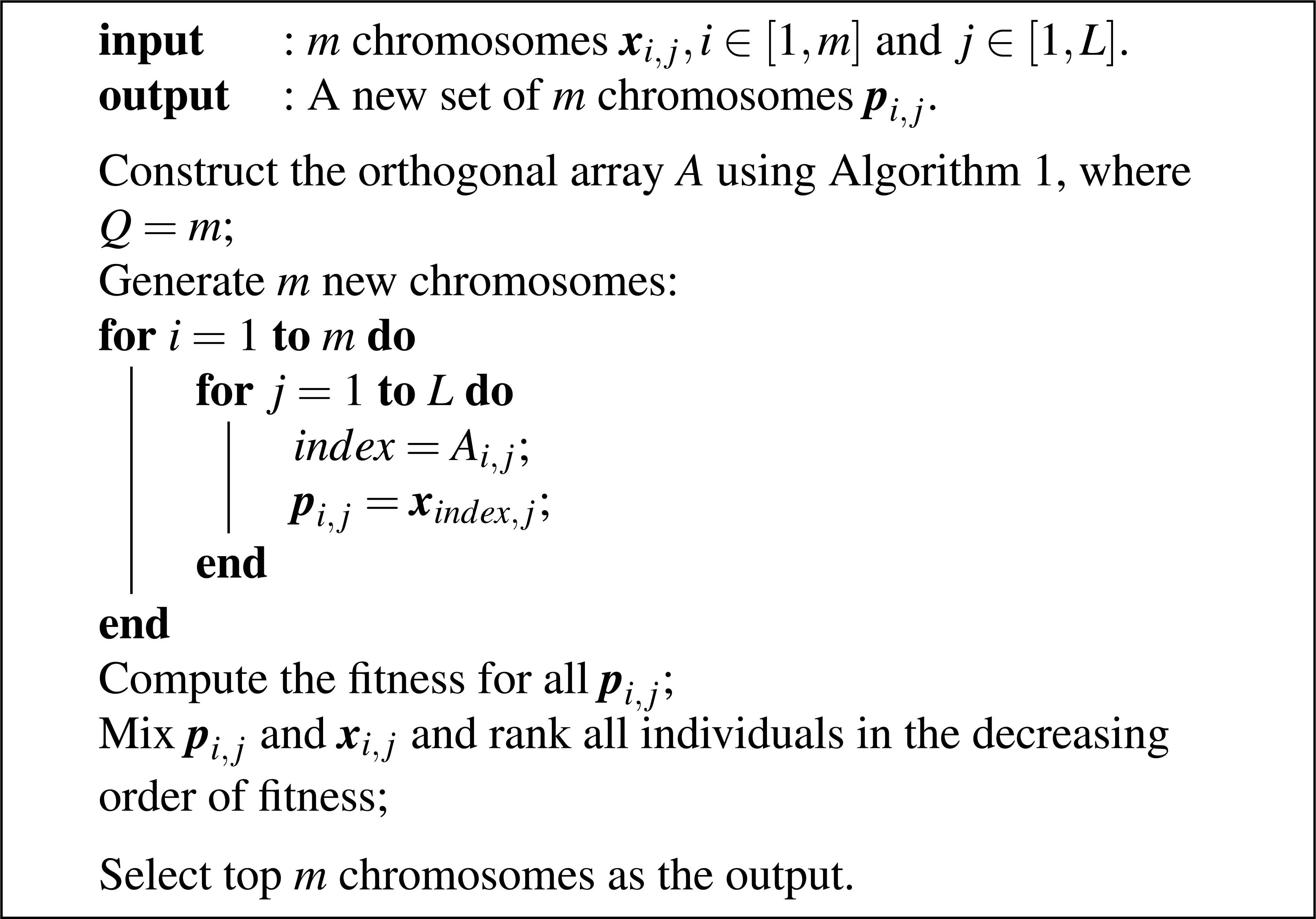
Orthogonal design based crossover operator for m chromosomes.
According to the OD method, the multiple-parent crossover operator considers each single character from selected chromosomes as one candidate factor. Then it scatters the candidate factors using the orthogonal array (as in Algorithm 1), and eventually generates m × m offspring. The advantage is two-fold. Firstly, the offspring are reproduced using multiple parents. That is, a more variety of genes is employed simultaneously to search for the better combination of gene factors. Secondly, rather than computing all possible combinations for candidate factors, the computational cost is reduced significantly based on OD, using only a subset of the full combinations.
We further consider an efficient way to compute the number m of selected chromosomes for the crossover operator. On one hand, with more selected chromosomes (a larger m), the crossover operator has a higher possibility of finding new combination, thereby improving the gene structure as well as the diversity. The disadvantage is that a higher-dimensional orthogonal array will be constructed which requires the additional computation. On the other hand, fewer selected chromosomes (a smaller m) will be less efficient to generate the new combination, even if less computation is need.
Herein the value of m is computed according to the average fitness value favg from the entire population and the fitness fbest from the best individuals. More precisely, if the favg value is much smaller than the fbest, then more chromosomes are required to search for better gene pattern to accelerate the convergence of the algorithm. Nevertheless, if the value of favg is close to fbest, which indicates the entire population starts to converge. Thus, fewer chromosomes are required to prevent gene structures from being removed.
Furthermore, we also need to ensure that the dimension of the orthogonal array matches the length of the chromosome, i.e., m + 1 ≥ L = 2 × h + 1, or m ≥ 2 × h. Overall, the number of selected chromosomes for the proposed crossover is calculated as follows:
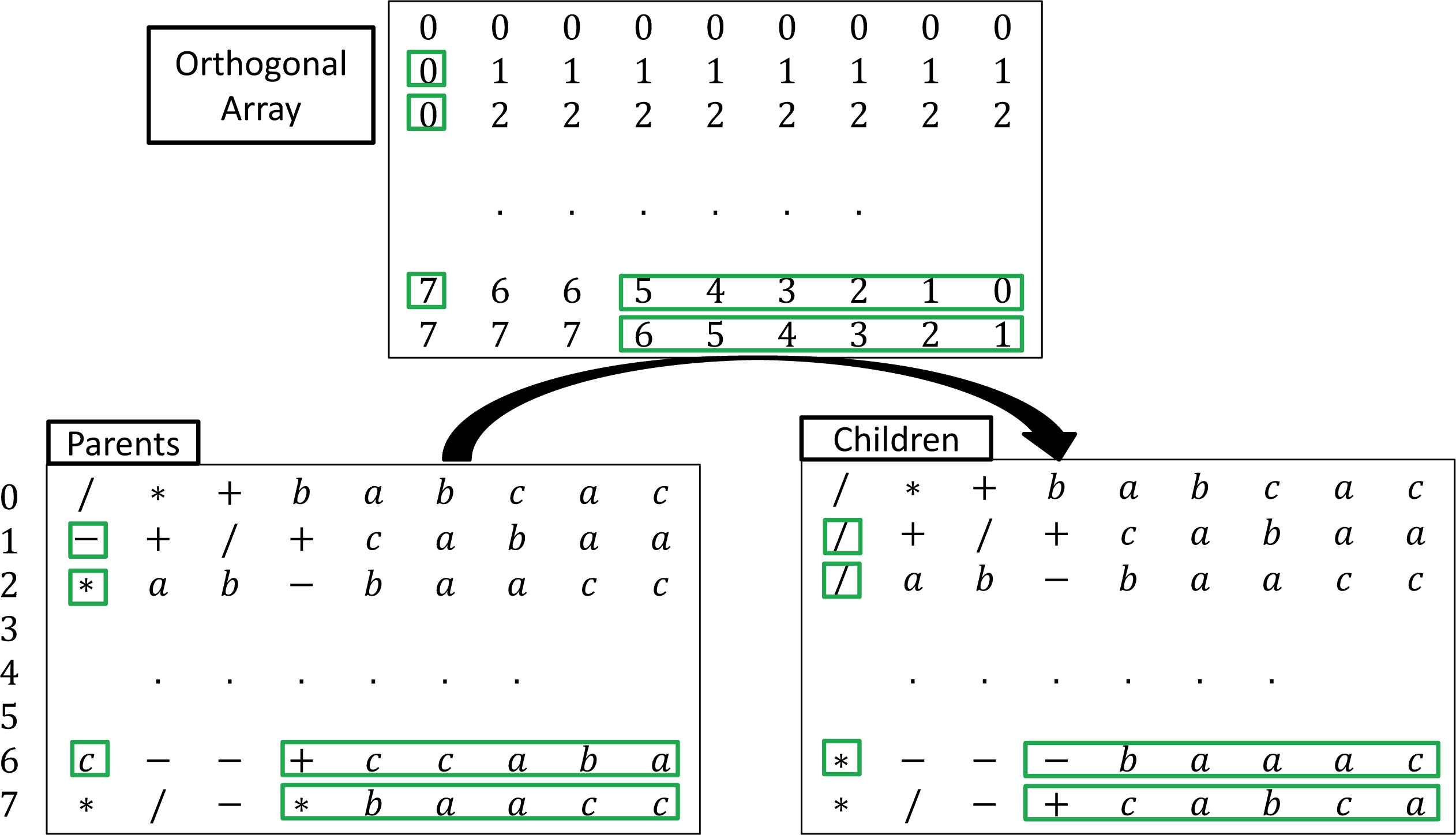
Demo of multiple-parent crossover operation using 8-parent chromosomes. Genes within green boxes indicates the crossover operation.
3.3. Evolutionary stable strategy
In conventional GEP algorithm, the generating-and-updating or the survival of the fittest strategy is applied. Consequently, the individual with high fitness will be selected for the next generation, while those with low fitness will be eliminated. As the evolution continues, the chromosomes with high fitness will dominate the entire population. Consequently, this conventional updating strategy may reduce the population diversity and lead to the premature convergence.
To address the premature problem while improving the diversity, the evolutionary stable strategy (ESS) is employed in this paper to monitor the evolution. The ESS is a balancing strategy in which the population cannot be invaded by a mutant strategy through the operation of natural selection 8,26. More precisely, with ESS it is implemented by always keeping a certain amount of low-fitness chromosomes in the population. Those individuals are used to provide additional gene structures and prevent best chromosomes from dominating the population.
Based on the concept of ESS, a stable factor δ is introduced to measure the stability of the population using the number of best individual chromosomes. If the ratio of best chromosomes exceeds a certain threshold, we then consider the population unstable and replace the extra best individuals with new chromosomes. As a result, the proposed strategy not only keeps the number of best individuals at a certain level, but also refresh the population with new genes to enhance the diversity. In this paper, the δ value is computed as follows:
3.4. Steps of the OGEP algorithm
In summary, the procedure of the OGEP algorithm is shown in Algorithm 3. The maximum iteration is used as the termination condition.
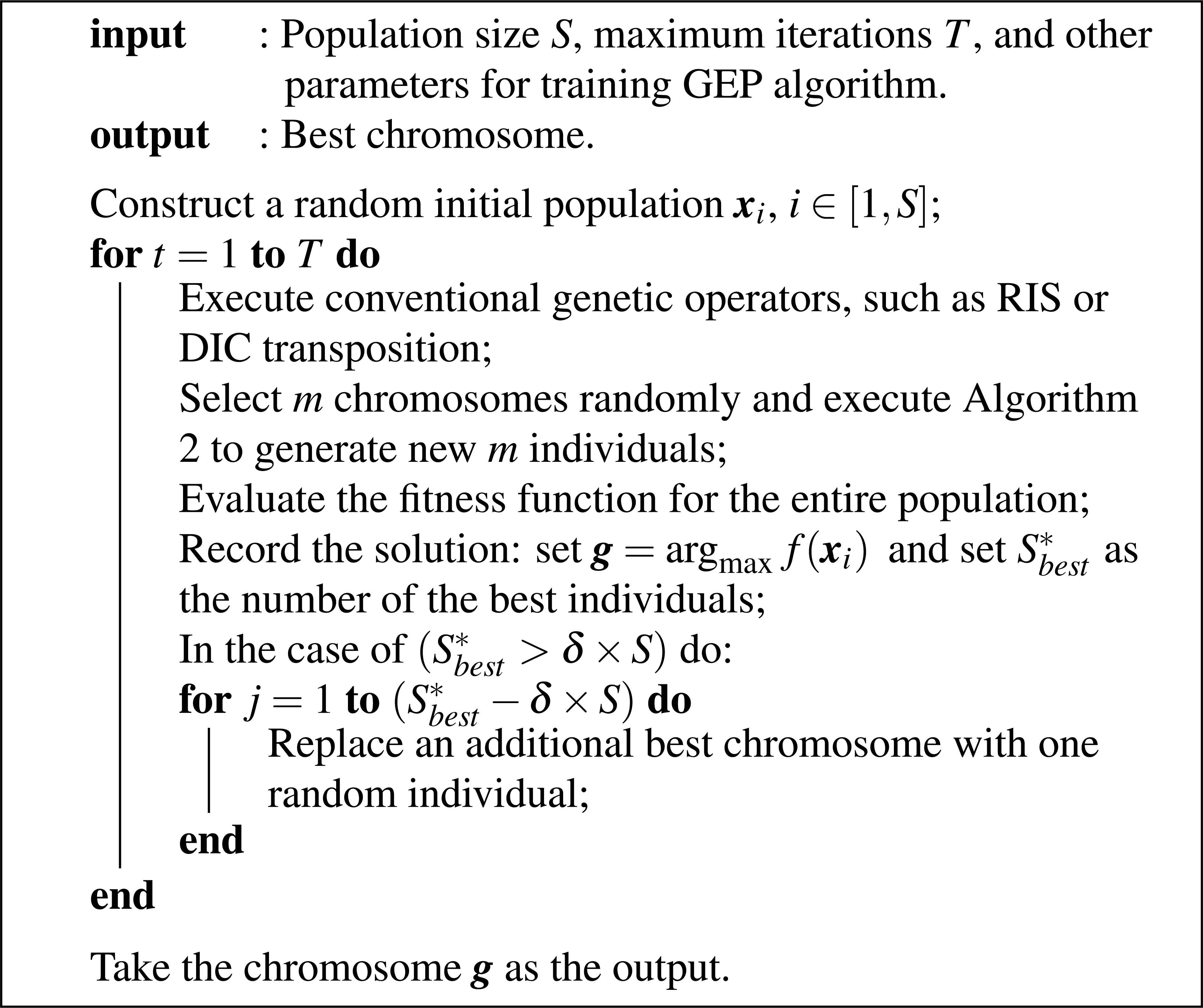
The procedure of the orthogonal gene expression programming algorithm.
4. Experimental result
This section presents the experimental results and comparison of the proposed OGEP algorithm with other conventional methods. We employ three real-world problems. The experimental data sets, parameters for OGEP and the evaluation criterion are presented in Section 4.1. The comparison between the proposed algorithm and traditional methods is presented in Section 4.2.
4.1. Experimental setup
Three real-world problems are chosen for experimental evaluation, which covers continuous and binary samples, a variety of numbers of input attributes, and diversity in different domains. The first problem is to formulate a prediction model for the electricity demand in Thailand from 1986 to 2010 25,16,22,23. The sample includes four input attributes, and the electricity consumption is the final output. The second problem is the estimation of plastic rotation capacity 5,13. In the production environment, the movement redistribution in a steel structure greatly depends on the rotation capacity of the plastic. Herein, the proposed algorithm is employed to estimate the relationship between the rotation capacity and other properties of the steel beam. The third problem is to predict the trend of the sunspot number time series 24. In this case, 100 annual observations of the Wolfer sunspots series from 1770 to 1869 is employed. Meanwhile, the sliding window method is applied to formulate the input and output data samples. More precisely, by continuously sliding a time-frame window with a given length (l) along the time axis, the input data is produced using the previous l data samples and the output sample is the (l +1)-th data. In this paper, the length of the time-frame l is set as ten.
All three data sets are partitioned into two subsets: a training set and a test set. The training set is used to train and optimize the algorithms. The test set is used for evaluation of the generalization ability. The size of the training and test sets in all cases is 75% and 25%, respectively.
For the proposed OGEP algorithm, the training parameters are set in Table 1. The training terminates when the maximum number of iterations is reached.
| Parameters | Details |
|---|---|
| Function sets | +,-,×, /, sin,cos,tan,√,log |
| Terminal sets | independent variables) |
| Population size | 100 | Crossover rate | 0.67 |
| Head length | 6 | Mutation rate | 0.03 |
| Linking function | + | Generations | 1000 |
| DC transposition rate | 0.11 | Number of genes | 5 |
| RIS transposition rate | 0.11 | Stable factor (δ) | 0.5 |
Parameters for OGEP algorithms.
The solution accuracy is evaluated using R-square, which is calculated as follows:
4.2. Performance analysis of the OGEP algorithm
In this section, the proposed OGEP algorithm is compared with conventional algorithms. We first apply the OGEP algorithm to solve the prediction problem for the electricity demand. There are in total 24 pairs of the data samples, each of which consists of four input and one output attributes. The statistics for the data samples are shown in Table 2.
| Attributes | Min | Max | Mean |
|---|---|---|---|
| annual population | 52511000 | 66903000 | 60769357.7 |
| GDP | 1257177 | 4364833 | 2962782 |
| stock index | 207.2 | 1682.9 | 687.2 |
| revenue | 364017.3 | 5149902.8 | 2215265.6 |
| consumption | 10162.7 | 60266.3 | 36316.3 |
Statistics for data samples used in the prediction model for the electricity demand.
Four variables, i.e., annual population, GDP, stock index, and revenue, are used as the input attributes while the consumption is the final output. Furthermore, all the input and output attributes are normalized to a range of [0.05,0.95] using the following equation:
Existing algorithms, including standard GEP 25, hybrid genetic programming-simulated annealing (GSA) 23, neural network (NN) 22 and multiple linear regression (MLR) 16, are employed for the comparison purpose. Table 3 presents the average approximation accuracy of the proposed algorithm and conventional methods over 30 runs.
| Algorithms | Training | Test |
|---|---|---|
| OGEP | 0.990 | 0.979 |
| GEP | 0.987 | 0.955 |
| GSA | 0.971 | 0.933 |
| NN | 1.0 | 0.966 |
| MLR | 0.992 | 0.933 |
Comparison of various prediction models for the electricity demand.
A few observation can be made from the simulation results. Firstly, the proposed OGEP algorithm achieves the best generalization ability in the test data set (R=0.979), which is better than other three conventional algorithms. Secondly, NN achieves the best approximation result for the training samples, however its generalization ability is worse than the proposed OGEP algorithm. The phenomenon can be explained that the neural network overfits the training samples which leads to a worse approximation performance for the test set. The best chromosome obtained by OGEP is shown in Figure 4.

The best chromosome for the electricity demand in OGEP.
The chromosome later is encoded as follows:
In the second case, we investigate the estimation problem of plastic rotation capacity for wide flange beams. There are in total 77 groups of data samples. Each sample consists seven input attributes: half length of flange (bmm), height of web (dmm), thickness of flange (t fmm), thickness of web (twmm), length of beam (Lmm), yield strength of flange (FyfMPa), and yield strength of web (FywMPa). Table 4 presents the descriptive statistics of the input attributes. For simplicity, all the input attributes are then scaled to a range of [1,10] by dividing 10 or 100.
| Attributes | bmm | dmm | t fmm | twmm |
|---|---|---|---|---|
| Minimun | 36.9 | 120.3 | 1.4 | 4.0 |
| Maximum | 150.4 | 320.0 | 17.3 | 11.5 |
| Average | 91.1 | 221.0 | 10.5 | 7.0 |
| Attributes | Lmm | FyfMPa | FywMPa | |
|---|---|---|---|---|
| Minimun | 960.0 | 236.0 | 217.0 | |
| Maximum | 4000.0 | 817.0 | 990.0 | |
| Average | 2659.8 | 353.4 | 404.5 |
Statistics of data samples for the estimation problem of plastic rotation capacity.
Table 5 reports the average approximation accuracy for various algorithms, such as conventional GEP 5 and neural networks 13, over 30 independent runs. As seen from the simulation results, the proposed OGEP method outperforms other algorithms in terms of both the training and test set. On average, the OGEP achieves a solution accuracy of 0.869 on the test sets, which is better than the accuracy of GEP (0.810) and NN (0.812) methods. The best chromosome obtained by OGEP is shown in Figure 5.

The best chromosome for the estimation problem of plastic rotation capacity.
| Algorithms | Training | Test |
|---|---|---|
| OGEP | 0.925 | 0.869 |
| GEP | 0.891 | 0.810 |
| NN | 0.903 | 0.812 |
Comparisons between the proposed OGEP algorithm and other approximation methods for the formulation model of rotation capacity in wide flange beams.
The chromosome further is explained as the following equation:
In the last example, the data for the Wolfer sunspots series from 1770 to 1869 (100 observations) is employed. The historical data shows that a circle occurred approximately every 10 years as time passes by. However, there was no repeated pattern over time in terms of the peak value. To analysis the trend of the Wolfer sunspots, the OGEP algorithm is employed by comparing with different methods, such as the standard GEP, GEP variant methods (GEP-RNC) 32, and symbolic GEP (SGEP) algorithm 24.
The simulation is run over 30 times and the average result is summarized in Table 6. As observed, OGEP outperforms its counterwork by generating the best perdition accuracy from either the training or test set. For instance, the proposed method improves 0.107%, 0.206%, 0.03% accuracy on average in terms of the generalization ability compared to the standard GEP, GEP-RNC, SGEP-based algorithms, respectively. The best chromosome obtained by OGEP is shown in Figure 6.

The best chromosome for estimating the trend of the Wolfer sunspots series.
| Algorithms | Training | Test |
|---|---|---|
| OGEP | 0.927 | 0.919 |
| GEP | 0.873 | 0.812 |
| GEP-RNC | - | 0.713 |
| SGEP | - | 0.889 |
Comparisons between the proposed OGEP algorithm and other GEP-based methods for the Wolfer sunspots series.
As a result, the chromosome from Figure 6 is translated into the following equation:
In conclusion, it can be empirically confirmed that the orthogonal design based operator and evolutionary stable strategy improves the performance of the standard GEP algorithm. In all three problems, the proposed algorithm outperforms the conventional GEP algorithm and its variant methods, such as GEP-RNC and SGEP. Meanwhile, the OGEP algorithm is comparable against other traditional algorithms, such as neural network and multiple linear regression model. The experimental results give us the strong evidence.
5. Conclusion
We have presented a novel gene expression programming algorithm using orthogonal design. Similar to other evolutionary algorithms, the OGEP algorithm makes a full use of the entire population to search for the best solution via different genetic operators. The main contribution is to introduce the orthogonal design based crossover to reproduce the offspring and employ evolutionary stable strategy to monitor the evolution.
The proposed operator is a multiple-parent crossover, which allows more than two chromosomes to reproduce the new gene combination. Meanwhile, the OD-based crossover can generate the candidate offspring uniformly over the search space and then select a representative subset. It results in more efficient information exchange among different individuals. Furthermore, an evolutionary stable strategy is also employed during the ongoing evolution. This strategy has been used to control the number of the best chromosomes while maintaining the population diversity. Evaluated on three benchmark datasets, the proposed OGEP algorithm is shown to outperform GEP-based variant and conventional optimization algorithms in terms of the generalization ability.
References
Cite this article
TY  - JOUR
AU  - Jie Yang
AU  - Jun Ma
PY  - 2016
DA  - 2016/08/01
TI  - A hybrid gene expression programming algorithm based on orthogonal design
JO  - International Journal of Computational Intelligence Systems
SP  - 778
EP  - 787
VL  - 9
IS  - 4
SN  - 1875-6883
UR  - https://doi.org/10.1080/18756891.2016.1204124
DO  - 10.1080/18756891.2016.1204124
ID  - Yang2016
ER  -