International Journal of Computational Intelligence Systems

Volume 9, Issue 5, September 2016, Pages 945 - 956

Existence and p-exponential stability of periodic solution for stochastic shunting inhibitory cellular neural networks with time-varying delays

Authors
Changjin Xu1, *, xcj403@126.com, Maoxin Liao2, maoxinliao@163.com, Yicheng Pang3, ypanggy@outlook.com
1Guizhou Key Laboratory of Economics System Simulation, Guizhou University of Finance and Economics, Guiyang 550004, PR China
2School of Mathematics and Physics, University of South China, Hengyang 421001, PR China
3School of Mathematics and Statistics, Guizhou University of Finance and Economics, Guiyang 550004, PR China
* Corresponding author, Email: xcj403@126.com (C.Xu).
Corresponding Author
Changjin Xuxcj403@126.com
Received 31 October 2014, Accepted 20 June 2016, Available Online 1 September 2016.
DOI
10.1080/18756891.2016.1237192How to use a DOI?
Keywords
Stochastic shunting inhibitory cellular neural networks; periodic solution; p-exponential stability; delay
Abstract

In this paper, we investigate a class of stochastic shunting inhibitory cellular neural networks with time-varying delays. Applying integral inequality, some sufficient conditions on the existence and p-exponential stability of periodic solutions for stochastic shunting inhibitory cellular neural networks with time-varying delays are established. An example is presented to illustrate our main theoretical findings. Our results are new and complementary to previously known studies.

Copyright
© 2016. the authors. Co-published by Atlantis Press and Taylor & Francis
Open Access
This is an open access article under the CC BY-NC license (http://creativecommons.org/licences/by-nc/4.0/).

1. Introduction

Since shunting inhibitory cellular neural networks have been successfully applied to pattern recognition, image and signal processing, vision, and optimization, their dynamics has attracted many attentions. Numerous important results on the existence and uniqueness of equilibrium point, periodic solution, almost periodic solution, pseudo almost periodic solution, almost automorphic solution and antiperiodic solution have been reported. For example, Gao et al.1 studied the existence and stability almost periodic solutions for cellular neural networks with time-varying delays in leakage terms on time scales, Liu and Shao2 analyzed the almost periodic solutions for SICNNs with time-varying delays in the leakage terms, Liu3 focused on the pseudo almost periodic solutions for neutral type CNNs with continuously distributed leakage delays, Armmaret al.4 made a detailed discussion on the existence and uniqueness of pseudo almost periodic solutions of recurrent neural networks with time-varying coefficients and mixed delays, Abbas and Xia5 investigated the almost automorphic solutions of impulsive cellular neural networks with piecewise constant argument, Li and Shu6 dealt with the antiperiodic solutions to impulsive shunting inhibitory cellular neural networks with distributed delays on time scales. For details, we refer readers to papers7,8,9,10,11,12,13,14.

In 1994, Haykin15 pointed out that in real nervous systems, synaptic transmission is a noisy process brought on by random fluctuations from the release of neurotransmitters and other probabilistic causes. Neural networks could be stabilized or destabilized by some stochastic inputs16. Considering that neural networks are inevitably affected by the random fluctuations from the release of neurotransmitters and other probabilistic causes which is an important component in neural networks, we think that it is worth while to investigate the stochastic neural networks. Recently, there are many papers that deal with this aspect17,18,19,20,21. In this paper, we will consider the following stochastic shunting inhibitory cellular neural networks with timevarying delays

dxij(t)=[aij(t)xij(t)+Lij(t)BklNr(i,j)Bijkl(t)fij(t,xkl(t))xij(t)CklNr(i,j)Cijkl(t)gij(t,xkl(tτkl(t)))xij(t)]dt+DklNr(i,j)Dijkl(t)σij(xij(t))dwij(t),tt0,
where i = 1,2, ⋯, m, j = 1,2, ⋯, n, τij(t) > 0 denotes axonal signal transmission delay at time t, Cij(t) denotes the cell at the (i, j) position of the lattice at time t, the r-neighborhood Nr(i, j) of Cij(t) is given as Nr(i,j)={Cijkl:max(|ki|,|lj|r),1km,1ln} , xij(t) stands for the activity of the cell Cij(t), Lij(t) denotes the external input to Cij(t), aij(t) > 0 stands for the passive decay rate of the cell activity, Bijkl(t)0 and Cijkl(t)0 represent the connection or coupling strength of postsynaptic of activity of the cell transmitted to the cell Cij(t) at time t and tτkl(t), respectively, the activity functions fij(t, xkl(t)) and gij(t, xkl(t)) are continuous functions representing the output or firing rate of the cell Ckl(t) at time t and tτkl(t), respectively, w(t) = (w11(t),w12(t), ⋯, wmn(t))T is m × n-dimensional Brownian motions defined on a complete probability space, σijC(R,R) is a Borel measurable function and σ = (σij)mn×mn is a diffusion coefficient matrix.

Let Rn(R+n) be the space of n-dimensional (non-negative) real column vectors and Rmn be the space of m × n-dimensional real column vectors. We denote (Ω, F, {Ft}t≥0, P) by a complete probability space with a filtration {Ft}t≥0, where F is a σ-algebra on a given set Ω, P is the probability measure and the filtration Ftt. satisfies the usual conditions, that is, {Ft}t≥0 is right continuous and F0 contains all P-null sets. Denote by BCF0b(R,Rmn) the family of bounded F0-measurable, Rmn valued random variables x(t), that is, the value of x(t) is an m × n-dimensional real vector and can be decided from the values of w(s) for s ≤ 0. Then BCF0b(R,Rmn) is a Banach space with the norm ||x||=sup0tω(E|x(t)|1p)1p, where p > 1 is an integer, |x(t)|1 = max(i,j)|xij(t)|, and E(.) stands for the correspondent expectation operator with respect to the given probability measure P. For convenience, for an ω-periodic continuous function f : RR, denote f = max0≤tω | f (t)|, f = min0≤tω | f (t)|, for any ϕBCF0b([τ,0],Rmn), denote [ϕ(t)]τ+=(|ϕ11|τ,|ϕ12|τ,,|ϕmn|τ)T, where |φij|τ = supτs≤0 |φij(t + s)|, i = 1,2, ⋯, m, j = 1,2, ⋯, n.

The initial value of system (1) takes the form

xij(s)=φij(s),s[t0τ,t0],
where φij(s)BCF0b([t0τ,0],R),τ=max1km,1ln{τkl},t0R.

Throughout this paper, we make the assumption as follows.

  • (H1) For i = 1,2, ⋯, m, j = 1,2, ⋯, n, aij(t), Bijkl(t), Cijkl(t), Dijkl(t) and Lij(t) are all ω-periodic continuous functions for all tR.

  • (H2) For i = 1,2, ⋯, m, j = 1,2, ⋯, n, there exist positive constants Lijf, gijg, σijσ, Mf and Mg such that

    |fij(t,u)fij(t,v)|Lijf|uv|,|fij(u)|Mf,|gij(t,u)gij(t,v)|Lijg|uv|,|gij(u)|Mg,|σij(t,u)σij(t,v)|Lijσ|uv|
    for all u, v, tR.

The remainder of the paper is organized as follows: in Section 2, several definitions and some preliminary results which are useful in later section are introduced. some sufficient conditions for the the existence of periodic solutions of system (1) are derived in Section 3. In Section 4, the p-exponential stability of periodic solutions are analyzed. An examples are given to illustrate the feasibility and effectiveness of our results obtained in previous section in Section 5. A brief conclusion is drawn in Section 6.

2. Preliminaries

In this section, we shall recall several definitions and present some preliminary results which are necessary in later sections.

Definition 2.1 22

A stochastic process x(t) is said to be periodic with period ω if its finite-dimensional distributions are periodic with period ω, that is, for any positive integer m and any moments of time t1, t2, ⋯, tm, the joint distribution of the random variables x(t1 + ), x(t2 + ), ⋯, x(tm + )) are independent of k, k = ±1, ±2, ⋯.

Lemma 2.1 23

If x(t) is an ω-periodic stochastic process, then its mathematical expectation and variance are ω-periodic.

Definition 2.2

A function x(t) = (x11(t), x12(t), ⋯, xmn(t))T defined on [t0τ, ∞) is said to be a solution of (1) with initial condition (2) if the following conditions holds.

  1. (i)

    xij(t) is absolutely continuous on [t0τ, ∞), i = 1,2, ⋯, m, j = 1,2, ⋯, n,

  2. (ii)

    xij(t) satisfies (1) for almost everywhere t ∈ [t0, ∞), i = 1,2, ⋯, m, j = 1,2, ⋯, n,

  3. (iii)

    xij(s) = φij(s), s ∈ [t0τ, t0], i=1,2, ⋯, m, j = 1,2, ⋯, n.

Throughout this paper, we assume that (1) with initial condition (2) has a unique solution. Denote the solution of (1) by x(t) = x(t, t0, φ) for all φBCF0b([t0τ,t0],Rmn) and t0R.

Definition 2.3 22

The solution x(t, t0, φ) of (1) is said to be

  1. (i)

    p-uniformly bounded, if for each α > 0, t0R, there exists a positive constant θ = θ (α) which is independent of t0 such that ||φ||pα implies E(x(t, t0, φ)||p) ≤ θ, tt0;

  2. (ii)

    p-point dissipative, if there exists a constant N > 0 such that for any point φBCF0b([τ,0],Rn), there exists T(t0, φ) such that E(||x(t, t0, φ)||p) ≤ N, tt0 + T(t0, φ).

Lemma 2.2 24

In addition to (H1) and (H2), suppose that the solution of (1) is p-uniformly bounded and p-point dissipative for p > 2, then (1) has an ω-periodic solution.

Lemma 2.3 25

For any xR+n and p > 0,

|x|pn(p21)0i=1nxip,(i=1nxi)pn(p1)0i=1nxip.

Definition 2.4 22

The periodic solution x(t, t0, φ) with initial value φBCF0b([τ,0],Rn) of (1) is said to be p-exponentially stable, if there are constants λ > 0 and M > 0 such that for any solution y(t, t0, φ1) with initial value φ1BCF0b([τ,0],Rn) of (1) satisfies

E(|xy|1p)M|varphiφ1||peλ(tt0),tt0.

Lemma 2.4 22

Let u(t)C(R,R+n) be a solution of the delay integral inequality

{u(t)M1eδ(tt0)[φ]τ++t0teC1(ts)A1u(s)ds+t0teC1(ts)B1[u(s)]τ+ds+J1,tt0,u(t)φ(t),t[t0τ,t0],
where A1, B1, C1, M1R+n×n, J1 ⩾ 0 is a constant vector, φ(t)C([tτ,t0],R+n). If ρ(Π) < 1, where Π=C11(A1+B1), then there are constants 0 < λδ and N ⩾ 1 such that
u(t)Nzeλ(tt0)+(IΠ)1J1,tt0,
where z satisfies [φ]τ+z.

Lemma 2.5 22

Assume that all conditions of Lemma 2.4 hold. If J1 = 0, then all solutions of inequality of (1) exponentially convergent to zero.

In view of Lemma 2.4 and Lemma 2.5, we have the following results.

Lemma 2.6 26

Let u(t)C(R,R+n) be a solution of the delay integral inequality

{u(t)M1eδ(tt0)[φ]τ++t0teC1(ts)A1u(s)ds+t0teC1(ts)B1[u(s)]τ+ds+J1,tt0,u(t)φ(t),t[t0τ,t0],
where A1, B1, C1, M1R+n×n, J1 ⩾ 0 is a constant vector, φ(t)C([tτ,t0],R+n). If A1+B1C1<1, then there are constants 0 < λδ and N ⩾ 1 such that
u(t)Nzeλ(tt0)+(1A1+B1C1)1J1,tt0,
where z satisfies [φ]τ+z. Moreover, if J1 = 0, then all solutions of the inequality of (4) are exponentially convergent to zero.

3. Existence of Periodic Solution

In this section, we discuss the existence of periodic solution of (1).

Theorem 3.1

In addition to (H1) and (H2), assume further that

(H3) there exists an integer p > 2 such that ρδ−1 < 1, where δ = min(i,j) {aij}, σ=(p(p1)2)p2,

ρ=max(i,j){5p1(a_ij)1p[(MfBklNr(i,j)B¯ijkl)p+(MgCklNr(i,j)C¯ijkl)p]+σ(mn)p2(2a_ij(p1)p2)1p2×(DklNr(i,j)D¯ijkl)p,
then (1.1) has an ω-periodic solution.

Proof

It follows from the method of variation parameter and (1) that for tt0, i = 1,2, ⋯, m, j = 1,2, ⋯, n,

xij(t)=xij(t0)et0taij(ξ)dξt0tet0taij(ξ)dξ[BklNr(i,j)Bijkl(s)fij(s,xkl(s))xij(s)+CklNr(i,j)Cijkl(s)gij(s,xkl(sτkl(s)))xij(s)Lij(s)]ds+t0tet0taij(ξ)dξDklNr(i,j)Dijkl(s)σij(xij(s))dwij(s).
Let
Θij(1)=xij(t0)e0taij(ξ)dξ,Θij(2)=t0tet0taij(ξ)dξBklNr(i,j)Bijkl(s)fij(s,xkl(s))xij(s)ds,Θij(3)=t0te0taij(ξ)dξCklNr(i,j)Cijkl(s)×gij(s,xkl(sτkl(s)))xij(s)ds,Θij(4)=t0tet0taij(ξ)dξLij(s)ds,Θij(5)=t0tet0taij(ξ)dξDklNr(i,j)Dijkl(s)σij(xij(s))dwij(s).
Taking expectations and applying Lemma 2.3, we get
E|xij(t)|pE(|Θij(1)|p+|Θij(2)|p+|Θij(3)|p+|Θij(4)|p+|Θij(5)|p),
where i = 1,2, ⋯, m, j = 1,2, ⋯, n. Next, we will evaluate every term of (6). For the first term of (6), we have
E|Θij(1)|p=xij(t0)et0taij(ξ)dξE|xij(t0)ea_ij(tt0)|pepa_ij(tt0)E|xij(t0)|p.

For the second term of (6), we have

E|Θij(2)|p=E|t0tet0taij(ξ)dξBklNr(i,j)Bijkl(s)fij(s,xkl(s))xij(s)ds|pE(t0tea_ij(ts)BklNr(i,j)B¯ijkl(s)|fij(s,xkl(s))|×|xij(s)|ds)pE(t0tea_ij(ts)BklNr(i,j)B¯ijkl(s)Mf|xij(s)|ds)p=E(t0t(ea_ij(ts))p1p(ea_ij(ts))1p×BklNr(i,j)B¯ijkl(s)Mf|xij(s)|ds)pE((t0tea_ij(ts)ds)p1t0tea_ij(ts)×(BklNr(i,j)B¯ijkl(s)Mf|xij(s)|)pds)(a_ij)1pt0tea_ij(ts)(MfBklNr(i,j)B¯ijkl)p×E||xij(s)|pds.

For the third term of (6), we have

E|Θij(3)|p=E|t0tet0taij(ξ)dξCklNr(i,j)Cijkl(s)gij(s,xkl(sτkl(s)))xij(s)ds|p=E(t0te0taij(ξ)dξCklNr(i,j)|Cijkl(s)||gij(s,xkl(sτkl(s)))||xij(s)|ds|p)E(t0tet0taij(ξ)dξCklNr(i,j)C¯ijklMg|xij(s)|ds)pE((t0teaij(ts)ds)p1t0teaij(ts)×(CklNr(i,j)C¯ijklMg|xij(s)|)pds)(a_ij)1pt0teaij(ts)(CklNr(i,j)C¯ijklMg)p×E|xij(s)|pds.

For the fourth term of (6), we get

E|Θij(4)|p=E|t0te0taij(ξ)dξLij(s)ds|pE|t0teaij(ts)Lij(s)ds|p(L¯ija_ij)p.

For the fifth term of (6), we get

E|Θij(5)|p=E|t0tet0taij(ξ)dξDklNr(i,j)Dijkl(s)σij(xij(s))dwij(s)|pσ[t0t(epa_ij(ts)×E|DklNr(i,j)(Dijkl(s))2σij2(xij(s))|p2)2pds]p2σ(mn)p2[t0t(epa_ij(ts)×E(DklNr(i,j)D¯ijkl|xij(s)|)p)2pds]p2=σ(mn)p2[t0t(e(p1)a_ij(ts)ea_ij(ts)×E(DklNr(i,j)D¯ijkl|xij(s)|)p)2pds]p2σ(mn)p2(t0te2a_j(p1)p2(ts)ds)p21×(t0tea_ij(ts)E(DklNr(i,j)D¯ijkl|xij(s)|)pds)σ(mn)p2(2a_ij(p1)p2)1p2×(t0tea_ij(ts)E(DklNr(i,j)D¯ijkl|xij(s)|)pds)σ(mn)p2(2a_ij(p1)p2)1p2×(t0tea_ij(ts)(DklNr(i,j)D¯ijkl)p×E|xij(s)|pds).

It follows from (8)(11) that

E|xij(t)|p5p1{epa_ij(tt0)E|xij(t0)|p+(L¯ija_ij)p+(a_ij)1pt0tea_ij(ts)(MfBklNr(i,j)B¯ijkl)pE||xij(s)|pds+(a_ij)1pt0teaij(ts)(MgCklNr(i,j)C¯ijkl)p×E|xij(s)|pds+σ(mn)p2(2a_ij(p1)p2)1p2×(t0tea_ij(ts)(DklNr(i,j)D¯ijkl)p×E|xij(s)|pds)}.
Define
V(t)=(v11(t),V12(t),,Vmn(t))T,
where Vij(t) = E|xij(t)|p, i = 1,2, ⋯, m, j = 1,2, ⋯, n. It follows from (12) that
Vij(t)5p1eδ(tt0)Vij(t0)+t0teδ(ts)Vij(s)ds+ι,
where l=max(i,j){(L¯ija_ij)p}. In view of (H3) and Lemma 2.4, we know that the solutions of (1) are p-uniformly bounded and the family of all solutions of (1) is p-point dissipative. By Lemma 2.2, we can conclude that (1) has an ω-periodic solution. The proof of Theorem 3.1 is completed.

4. p-exponential Stability of Periodic Solution

In this section, we will consider the p-exponential stability of periodic solutions of (1).

Theorem 4.1

In addition to (H1)-(H2), assume further that

(H4) there exists an integer p > 2 such that (ρ1 + ρ2)δ−1 < 1, where

ρ1=max(i,j){6p1((a_ij)1p[(MfBklNr(i,j)B¯ijkl)p+(NLijfBklNr(i,j)B¯ijkl)p]+σ(mn)p2(2a_ij(p1)p2)1p2×(DklNr(i,j)D¯ijkl)p)}
and
ρ2=max(i,j){6p1(a_ij)1p[(MgCklNr(i,j)C¯ijkl)p+(NLijgCklNr(i,j)C¯ijkl)p]},
then the periodic solution of (1) is p-exponentially stable.

Proof

Obviously, if (H4) holds, then (H3) is fulfilled. In view of Theorem 3.1, we know that (1) has an ω-periodic solution x*(t)={xij*(t)} with the initial condition φ(t) = {φij(t)}, i = 1,2, ·,m, j = 1,2, ⋯, n. Thus x*(t) is p-uniform, namely, there is a constant C0 > 0 such that E|xij*(t)|p<C0, i = 1,2, ·,m, j = 1,2, ⋯, n. Assume that x(t) = {xij(t) is an arbitrary solution of (1) with the initial condition ψ(t) = {ψij(t)}, i = 1,2, ·,m, j = 1,2, ⋯, n. Let

u(t)={uij(t)}={xij(t)xij*(t)},
where i = 1,2, ·,m, j = 1,2, ⋯, n. Then for i = 1,2, ·,m, j = 1,2, ⋯, n and tt0, we get
duij(t)=[aij(t)uij(t)BklNr(i,j)Bijkl(t)(fij(t,xkl(t))xij(t)fij(t,xkl*(t))xij*(t))CklNr(i,j)Cijkl(t)(gij(t,xkl(tτkl(t)))xij(t)gij(t,xkl*(tτkl(t)))xij*(t))]dt+DklNr(i,j)Dijkl(t)(σij(xij(t))σij(xij*(t)))dwij(t)
with this initial condition
ϕij(s)=ψij(s)φij(s),s[τ,t0],
where i = 1,2, ·, m, j = 1,2, ⋯, n. Applying the method of variation parameter, we have
uij(t)=uij(t0)e0taij(ξ)dξt0tet0taij(ξ)dξ×[BklNr(i,j)Bijkl(s)(fij(s,xkl(s))xij(s)fij(s,xkl*(s))xij*(s))+CklNr(i,j)Cijkl(s)(gij(s,xkl(sτkl(s)))xij(s)gij(s,xkl*(sτkl(s)))xij*(s)]ds+t0tet0taij(ξ)dξDklNr(i,j)Dijkl(s)(σij(xij(s))σij(xij*(s)))dwij(s)=uij(t0)e0taij(ξ)dξt0te0taij(ξ)dξ×[BklNr(i,j)Bijkl(s)(fij(s,xkl(s))uij(s)(fij(s,xkl(s))fij(s,xkl*(s))xij*(s))+CklNr(i,j)Cijkl(s)(gij(s,xkl(sτkl(s)))uij(s)+(gij(s,xkl(sτkl(s)))gij(s,xkl*(sτkl(s))))xij*(s))]ds+t0tet0taij(ξ)dξDklNr(i,j)Dijkl(s)(σij(xij(s))σij(xij*(s)))dwij(s),
where i = 1,2, ·, m, j = 1,2, ⋯, n and tt0. Let
Φij(1)=uij(t0)e0taij(ξ)dξ,Φij(2)=t0tet0taij(ξ)dξ×BklNr(i,j)Bijkl(s)fij(s,xkl(s))uij(s)ds,Φij(3)=t0tet0taij(ξ)dξBklNr(i,j)Bijkl(s)×(fij(s,xkl(s))fij(s,xkl*(s))xij*(s)ds,Φij(4)=t0tet0taij(ξ)dξ×CklNr(i,j)Cijkl(s)gij(s,xkl(sτkl(s)))uij(s)ds,Φij(5)=t0tet0taij(ξ)dξ×CklNr(i,j)Cijkl(s)(gij(s,xkl(sτkl(s)))gij(s,xkl*(sτkl(s))))xij*(s)ds,Φij(6)=t0tet0taij(ξ)dξ×DklNr(i,j)Dijkl(s)(σij(xij(s))σij(xij*(s)))dwij(s).
Taking expectations and applying Lemma 2.3, we have
E|uij(t)|p6p1E(|Φij(1)|p+|Φij(2)|p+|Φij(3)|p+|Φij(4)|p+|Φij(5)|p+|Φij(6)|p).
where i = 1,2, ⋯, m, j = 1,2, ⋯, n. Applying the similar method in the proof of Theorem 3.1, we get
E|Φij(1)|pepa_ij(tt0)E|uij(t0)|pE|Φij(2)|p=E|t0tet0taij(ξ)dξ×BklNr(i,j)Bijkl(s)fij(s,xkl(s))uij(s)ds|p(a_ij)1pt0tea_ij(ts)(MfBklNr(i,j)B¯ijkl)p×E||uij(s)|pds,E|Φij(3)|pE|t0tet0taij(ξ)dξ×BklNr(i,j)Bijkl(s)(fij(s,xkl(s))fij(s,xkl*(s))xij*(s)ds|pE(t0tea_ij(ts)×BklNr(i,j)B¯ijklC0Lijf|ukl(s)|ds)p(a_ij)1pt0tea_ij(ts)×(C0LijfBklNr(i,j)B¯ijkl)pE|ukl(s)|pds,E|Φij(4)|pE|t0te0taij(ξ)dξCklNr(i,j)Cijkl(s)×gij(s,xkl(sτkl(s)))uij(s)ds|p(a_ij)1pt0teaij(ts)(MgCklNr(i,j)C¯ijkl)pE||ukl(sτkl(s))|pds,E|Φij(5)|pE|t0tet0taij(ξ)dξCklNr(i,j)Cijkl(s)(gij(s,xkl(sτkl(s)))gij(s,xkl*(sτkl(s))))xij*(s)ds|p(a_ij)1pt0tea_ij(ts)×(C0LijgCklNr(i,j)C¯ijkl)p×E|ukl(sτkl(s))|pds,E|Φij(6)|pE|t0tet0taij(ξ)dξ×DklNr(i,j)Dijkl(s)(σij(xij(s))σij(xij*(s)))dwij(s)|pσ(mn)p2(2aij(p1)p2)1p2(t0tea_ij(ts)(DklNr(i,j)D¯ijkl)p×E|uij(s)|pds).
Then we have
E|uij|p6p1{epa_ij(tt0)E|uij(t0)|p+(a_ij)1pt0tea_ij(ts)(MfBklNr(i,j)B¯ijkl)p×E||uij(s)|pds+(a_ij)1pt0tea_ij(ts)(C0LijfBklNr(i,j)B¯ijkl)p×E|ukl(s)|pds+(a_ij)1pt0tea_ij(ts)(MgCklNr(i,j)C¯ijkl)p×E||ukl(sτkl(s))|pds+(a_ij)1pt0tea_ij(ts)(C0LijgCklNr(i,j)C¯ijkl)p×E|ukl(sτkl(s))|pds+σ(mn)p2(2a_ij(p1)p2)1p2(t0tea_ij(ts)(DklNr(i,j)D¯ijkl)p×E|uij(s)p|ds)}.
Define
W(t)=(W11(t),W12(t),,Wmn(t))T,
where Wij(t) = E|uij(t)|p, i = 1,2, ⋯, m, j = 1,2, ⋯, n. It follows from (19) that
Wij(t)6p1eδ(tt0)Wij(t0)+t0teδ(ts)ρ1Wij(s)dst0teδ(ts)ρ2|Wij(s)|τ+ds,
where
ρ1=max(i,j){6p1((a_ij)1p[(MfBklNr(i,j)B¯ijkl)p+(C0LijfBklNr(i,j)B¯ijkl)p]+σ(mn)p2(2a_ij(p1)p2)1p2×(DklNr(i,j)D¯ijkl)p)}
and
ρ2=max(i,j){6p1(a_ij)1p[(MgCklNr(i,j)C¯ijkl)p+(C0LijgCklNr(i,j)C¯ijkl)p]}.
In view of (H4) and Lemma 2.5, we can conclude that the periodic solution x*(t) of (1) is pexponentially stable. The proof of Theorem 4.1 is completed.

Remark 4.1

In Zhao and Zhang27, Zhao and Zhang investigated the almost periodic solution of the following shunting inhibitory cellular neural networks with variable coefficients and time-varying delays

x˙ij(t)=aij(t)xij(t)BklNr(i,j)Bijkl(t)fij(t,xkl(t))xij(t)CklNr(i,j)Cijkl(t)gij(t,xkl(tτkl(t)))xij(t)+Lij(t).
By applying Dini derivative, they established some criteria on the existence and local exponential stability of (22). All the results in Zhao and Zhang27 can not be applicable to system (1) to obtain the the existence and p-exponential stability of periodic solutions. This implies that the results of this article are essentially new.

5. An Example with Its Numerical Simulations

Example 5.1

Let i = j = 2. Consider the following stochastic shunting inhibitory cellular neural networks with time-varying delays

dxij(t)=[aij(t)xij(t)+Lij(t)BklNr(i,j)Bijkl(t)fij(t,xkl(t))xij(t)CklNr(i,j)Cijkl(t)gij(t,xkl(tτkl(t)))xij(t)]dt+DklNr(i,j)Dijkl(t)σij(xij(t))dwij(t),
where fij(t,x)=sin15x+45x, gij(t,x)=sin13x+23x and
[a11(t)a12(t)a21(t)a22(t)]=[0.3+0.02cosπ2t0.4+0.02sinπ2t0.4+0.01cosπ2t0.3+0.01cosπ2t],[B11(t)B12(t)B21(t)B22(t)]=[0.02|cosπ4t|0.03sinπ4t0.01sinπ4t0.02cosπ4t],[C11(t)C12(t)C21(t)C22(t)]=[0.03|sinπ4t|0.03cosπ4t0.02cosπ4t0.02sinπ4t],[D11(t)D12(t)D21(t)D22(t)]=[0.02|cosπ4t|0.01sinπ4t0.01cosπ4t0.02sinπ4t],[L11(t)L12(t)L21(t)L22(t)]=[0.2cosπ2t0.1sinπ2t0.3cosπ2t0.2sinπ2t],[σ11(u)σ12(u)σ21(u)σ22(u)]=[0.2sinu0.2sinu0.2cosu0.1sinu],[τ11(t)τ12(t)τ21(t)τ22(t)]=[0.01|sint|0.02|cosu|0.02|sinu|0.01|cosu|].
Then Lij f = Lijg = Mf = Mg = 1(i, j = 1,2), τ = 0.02, L11σ = L22σ = 0.1, L12σ = L21σ = 0.2 and
[BklN1(1,1)B¯11klBklN1(1,2)B¯12klBklN1(2,1)B¯21klBklN1(2,2)B¯22kl]=[0.080.120.040.08],[CklN1(1,1)C¯11klCklN1(1,2)C¯12klBklN1(2,1)C¯21klCklN1(2,2)C¯22kl]=[0.120.120.080.08],[a_11a_12a_21a_22]=[0.280.380.390.29],[L¯11L¯12L¯21L¯22]=[0.20.10.30.2].
Take p = 3, r = 1. Then we have δ ≈ 0.2302, σ1 ≈ 0.0704, σ2 ≈ 0.0462. It is easy to check that all the conditions in Theorem 3.1 and Theorem 4.2 are fulfilled. Hence we can conclude that then (23) has a 4-periodic solution, which is 3-exponentially stable. The results are shown in Figs. 12.

Fig. 1.

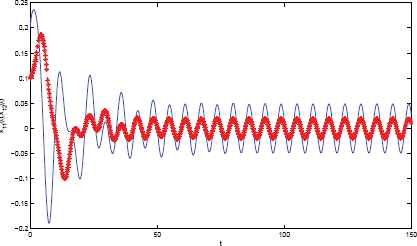
Transient response of state variables x11(t) and x12(t), where the blue line stands for x11(t) and the red line stands for x12(t).

Fig. 2.

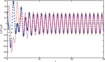
Transient response of state variables x21(t) and x22(t), where the blue line stands for x21(t) and the red line stands for x22(t).

6. Conclusions

In this paper, a class of stochastic shunting inhibitory cellular neural networks with time-varying delays are considered. We establish some sufficient conditions ensuring the existence and p-exponential stability of periodic solutions for stochastic shunting inhibitory cellular neural networks with timevarying delays by using integral inequalities. Comparisons between our results and the previous results show that our results complement the earlier publications and are completely new. An example is presented to illustrate our main theoretical findings. Our results play an important key in designing of shunting inhibitory cellular neural networks. The obtained results show that under some appropriate circumstances, stochastic shunting inhibitory cellular neural networks with time-varying delays can display sustainable periodic oscillatory phenomenon. These periodic oscillatory phenomenon can help us to process visual information quickly and effectively28,29. Also periodic oscillatory phenomenon can be helpful for us to predict pathological brain states, which is important to diagnose disease in medical science30,31,32.

Acknowledgments

This work is supported by National Natural Science Foundation of China (No.61673008, No.11261010 and No.11526063), Natural Science and Technology Foundation of Guizhou Province(J[2015]2025 and J[2015]2026), 125 Special Major Science and Technology of Department of Education of Guizhou Province ([2012]011) and Natural Science Foundation of the Education Department of Guizhou Province(KY[2015]482).

References

Journal
International Journal of Computational Intelligence Systems
Volume-Issue
9 - 5
Pages
945 - 956
Publication Date
2016/09/01
ISSN (Online)
1875-6883
ISSN (Print)
1875-6891
DOI
10.1080/18756891.2016.1237192How to use a DOI?
Copyright
© 2016. the authors. Co-published by Atlantis Press and Taylor & Francis
Open Access
This is an open access article under the CC BY-NC license (http://creativecommons.org/licences/by-nc/4.0/).

Cite this article

TY  - JOUR
AU  - Changjin Xu
AU  - Maoxin Liao
AU  - Yicheng Pang
PY  - 2016
DA  - 2016/09/01
TI  - Existence and p-exponential stability of periodic solution for stochastic shunting inhibitory cellular neural networks with time-varying delays
JO  - International Journal of Computational Intelligence Systems
SP  - 945
EP  - 956
VL  - 9
IS  - 5
SN  - 1875-6883
UR  - https://doi.org/10.1080/18756891.2016.1237192
DO  - 10.1080/18756891.2016.1237192
ID  - Xu2016
ER  -