
An Effective Hybrid Differential Evolution Algorithm Incorporating Simulated Annealing for Joint Replenishment and Delivery Problem with Trade Credit
- DOI
- 10.1080/18756891.2016.1256567How to use a DOI?
- Keywords
- Joint Replenishment and Delivery; trade credit; hybrid differential evolution algorithm; simulated annealing algorithm
- Abstract
In practice, suppliers often provide retailers with forward financing to increase demand or decrease inventory. This paper proposes a new and practical joint replenishment and delivery (JRD) model by considering trade credit. However, because of the complex mathematical properties of JRD, high-quality solutions to the problem have eluded researchers. We design an effective hybrid differential evolution algorithm based on simulated annealing (HDE-SA) that can resolve this non-deterministic polynomial hard problem in a robust and precise way. After determining the suitable parameters by a parameter-tuning test, we verify the performance of the HDE-SA through numerical JRD examples. Compared with the results of other popular evolutionary algorithms, results of randomly generated JRDs indicate that HDE-SA can always obtain slightly lower total costs than differential evolution algorithm (DE) and genetic algorithm (GA) under different situations. Moreover, the convergence rate of the HDESA is higher than that of DE and GA. Thus, the proposed HDE-SA is a potential tool for the JRD with trade credit.
- Copyright
- © 2016. the authors. Co-published by Atlantis Press and Taylor & Francis
- Open Access
- This is an open access article under the CC BY-NC license (http://creativecommons.org/licences/by-nc/4.0/).
1. Introduction
Joint replenishment problem (JRP) has been heavily studied since the early work of Shu [1] was published. The JRP policy means that group items are ordered from the same supplier to achieve the target of sharing fixed ordering costs and saving procurement costs [2]. A corresponding review has been conducted by Khouja and Goyal [3]. Adopting a joint replenishment policy can result in cost savings, so managers are aware that using a joint replenishment and delivery (JRD) policy can obtain a scale effect of replenishment and transportation simultaneously, thereby further reducing total cost [4].
In practice, companies often use a JRD policy to earn larger profit. In 2013, as a branch of GEFCO (or “les Groupages Express de Franche Comté”, in French), Europe’s leading automotive industrial logistics service provider, Wuhan Dongfeng GEFCO Logistics Ltd. (WH-GEFCO) established a logistics partnership with Dongfeng Peugeot Citroen Automobile Co. Ltd. (DPCA) for an automobile spare parts regional distribution center (RDC) in Beijing City. As shown in Fig. 1, different kinds of spare parts from different suppliers are transported to a central warehouse in Wuhan City, and thereafter are transported to the RDC in other cities. Then, WH-GEFCO transported spare parts to more than 200 4S outlets. The deputy manager of DPCA said that the JRD policy was able to improve efficiency and reduce considerable cost.
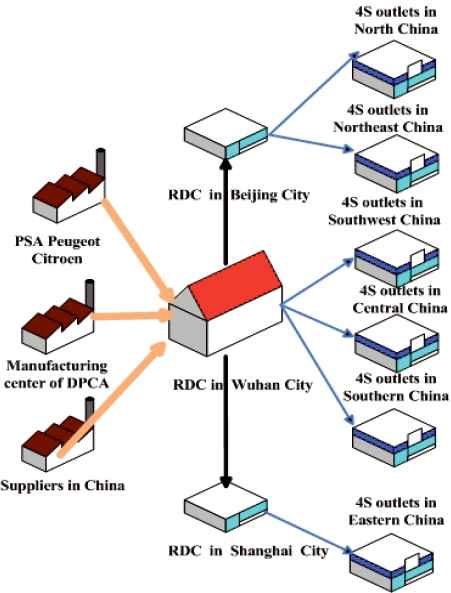
Logistics processes of automobile spare parts for DPCA
Unfortunately, the literature on JRD is limited. Cha, Moon, and Park [5] focused on the JRD of a one-warehouse, n-retailer system. A heuristic and an intelligent algorithm were proposed to solve this JRD. Moon, Cha, and Lee [6] developed joint replenishment and consolidated freight-delivery models and four efficient algorithms are used to resolve the models. Wang, Dun, et al. [4] proposed a two-level stochastic JRD by extending the model of Qu, Bookbinder, and Iyogun [7] and verified that the differential evolution algorithm is effective and efficient. Scholars have also developed several relevant extensions such as JRD under fuzzy environment [8], radio-frequency identification technology investment evaluation model of JRD [9], JRD with delivery constraint [10], location-inventory problem with joint replenishment policy [11], and JRD with multi-warehouse [12].
It is very popular that suppliers always provide the retailer a credit period to settle the amount owed for goods already supplied. For instance, Wal-Mart’s trade credit is eight times the amount of capital invested by its shareholders [13]. Lin, Ouyang, and Dang [14] proposed an integrated supplier–retailer inventory model considering trade credit policies and defective items. Zhong and Zhou [15] developed a model to determine the ordering or trade-credit policy of a supply chain. Considering JRPs with trade credit, Tsao [16] examined how to coordinate multi-echelon multi-item channels by analyzing two trade allowances, namely, effort cost sharing and cash discount within a credit period. Tsao and Teng [17] considered the JRP with trade credit by determining the optimal replenishment schedule for each item. The issue of trade credit is a highly popular research subject. Until now, only these two papers have investigated the JRPs under trade credits, and studies that focus on the JRDs under trade credits are not available.
The present study aims to develop a new and practical JRD model under trade credits for the first time and provide effective and reliable algorithms. The goal of this JRD policy is to determine the replenishment frequencies and delivery frequencies of items to minimize the total system cost.
However, we still face the difficult task of finding effective and efficient algorithms. JRDs have been proven to be NP-hard problems and designing high-quality algorithms is difficult. Current approaches include iterative algorithms, genetic algorithm (GA) [5], and differential evolution algorithm (DE) [4] [9]. Solving JRDs effectively by traditional approaches is obviously difficult for the following reasons: (1) Available heuristics are too problem-specific and difficult to design, and versatile approaches do not exist. (2) The enumeration is inefficient. Discovering an opposite solution for a large problem size may take years. (3) Classic GAs were verified as suitable approaches for JRPs. However, GAs sometimes show inherent defects that lead to stagnation and prematurity, and the calculated cost increases exponentially with the scale of the problem. Thus, finding effective approaches is necessary to solve the JRD with trade credit more accurately.
Among the metaheuristics, the DE is one of the best evolutionary algorithms in a variety of fields [18–20]. Thus, DEs are used to solve JRDs because of easy implementation, quick convergence, and robustness. However, the DE falls easily into local search whereas simulated annealing (SA) can avoid the disadvantage of local search for classic DE through the Metropolis criterion [21]. In fact, the hybrid method named DESA that combines DE and SA was recognized by scholars [22]. Olenšek, Tuma, Puhan, and Bűrmen [23] presented a new hybrid asynchronous parallel global optimization method–parallel simulated annealing differential evolution to optimize five real-world analog integrated circuits. This approach combines features from SA and DE to efficiently sample the parameter space. Zhang et.al [24] developed an SA-based multi-objective cultural DE to solve daily hydrothermal operation scheduling with economic emission. However, these modified hybrid algorithms were designed to address specific problems and could not be used to solve JRD with trade credit directly.
Thus, we extend the existing DESA by introducing the adaptive mutation factor, which decreases gradually with evolutionary generation. The large value in the initial period can rapidly explore possible solution space, and the small value in the later period can exploit the optimal solution in explored solution space. The new method is referred to as hybrid DE based on SA (HDESA). For better comparison, we also use basic DE and GA to resolve this non-deterministic polynomial hard (NP-hard) problem because they are other widely-used and good approaches for solving the similar problems. Results of contrastive examples and randomly generated problems illustrate that, compared with other algorithms, HDE-SA is more effective and robust in resolving this complex problem.
The rest of this paper is organized as follows. The assumptions and notations are described and the proposed model is formulated in Section 2. In Section 3, an HDE-SA is provided to resolve the proposed JRD. Computational and sensitivity analyses are presented in Section 4. Finally, conclusions and future research directions are drawn in Section 5.
2. Proposed new JRD with trade credit and analysis
2.1. Assumptions and notation
A JRD problem with trade credit, which is composed of a warehouse, n suppliers, and n retailers is considered as shown in Fig. 2. The warehouse replenishes multiple items from upstream suppliers to meet the demands of the retailers. The JRD policy aims to determine the replenishment frequencies and delivery frequencies of items to minimize the total system cost.
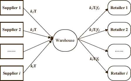
Description about the JRD with trade credit
The JRD in this study has the following assumptions similar to those in the study of Cha et al. [5]: (a) Demand rates and costs for these items are known and constant; (b) Shortages are not allowed; (c) Replenishments occur instantaneously; (d) The unit retail price of the products sold during the credit period is deposited in an interest bearing account with rate Ie. At the end of this period, the credit is settled and the retailer starts paying for interest charges for the items in stock with rate Ip.
The following notations are used:
N: number of items,
i : index of item, 1≤ i ≤ N,
pi : selling price per unit for item i,
ci : purchasing price per unit for item i,
di : demand rate for item i,
Sw: warehouse’s major ordering cost,
Ip : interest charged per dollar,
Ie : interest earned per dollar,
M : length of credit period,
T: basic cycle time for the warehouse,
ki: integer number that makes kiT the replenishment cycle time for item i (decision variable);
fi : integer number that determines the outbound delivery schedule of item i (decision variable)
θ: set of items with a replenishment cycle that is longer than or equal to the credit period; and
ϕ: set of items with a replenishment cycle that is shorter than the credit period.
2.2. Mathematical formulation and analysis
2.2.1 Related cost analysis
- (1)
The annual ordering cost of all items is:
This equation includes the annual major ordering cost (first term) and the annual minor ordering cost (second term). - (2)
The annual inventory holding cost of the warehouse is:
- (3)
The annual outbound transportation cost is:
- (4)
The annual inventory holding cost of the retailers is:
- (5)
The interest earned on each item is expressed as follows :
Case 1: for ki T / fi ≥ M
The annual interest earned is:
The total annual interest earned is the sum of the annual interest earned for item i ∈ θ. The unit retail price of the products sold during credit period M is deposited in an interest bearing account with rate Ie.
Case 2: for kiT /fi < M
The annual interest earned is:
The total annual interest earned is the sum of the annual interest earned for item i ∈ ϕ. Since the credit period is longer than the replenishment cycle time, the annual interest earned includes the interest earned before the replenishment cycle time
- (6)
The interest paid on each item is expressed as follows :
Case 1: for kiT / fi ≥ M
The annual interest paid is:
The total annual interest paid is the sum of the annual interest paid for item i ∈ θ. After M, the retailer starts paying the interest charges for the items still in stock with rate Ip.
Case 2: for kiT / fi < M
The annual interest paid is Cn=0. In this case, no interest is paid on the items because the credit period is longer than the replenishment cycle time.
2.2.2 Total annual cost
Based on the preceding discussion, the objective of the JRD is:
3. Proposed HDE-SA and procedures for the JRD with trade credit
3.1. Proposed HDE-SA
Although DE has been proven to be an effective and robust approach by utilizing the optimization of well-known non-linear, non-differentiable, and non-convex functions, it is also likely to fall into local search because of its one-to-one selection mechanism. Thus, the advantages of SA can be adopted to overcome the shortcoming of DE. The random sampling and the Metropolis criterion from SA are combined with the population of points and the sampling mechanism from DE to balance global and local search. Moreover, the values of mutation factor F and crossover factor CR have effects on the performance of the algorithm. An HDE-SA is proposed to obtain a more stable and effective algorithm.
The improvements are as follows: (a) we use SA to optimize the result obtained by HDE to overcome the shortcoming of one-to-one competing in the typical DE; and (b) the adaptive mutation factor F can maintain the balance between exploring and exploiting abilities. The main processes of HDE-SA are discussed as follows.
3.1.1 Mutation
The mutation operation produces a new vector by adding the weighted difference of two random vectors to a third vector. For each target vector
Unlike the constant F in original typical DE, we create F by Eq. (3), which decreases gradually with the evolutionary generation of HDE-SA. The large value at the initial stage can rapidly explore the possible solution space, and the small value at the later stage can exploit the optimal solution in the explored solution space.
3.1.2 Crossover
The crossover operation combines the mutated vectors and the target vectors to increase the diversity of the parameter vector. The trial vector can be obtained as:
3.1.3 Selection
Ultimately, after mutation and crossover operation, the selection operation generates the next generation by selecting between the trail vector and the corresponding target vector. The selection rule to minimize the function is as follows:
3.1.4 SA operation
After obtaining the result by HDE, a new vector is created through the following equation:
TGen is firstly equal to Temp, i.e. the maximum temperature; then, it changes according to the following equation:
SA operation is stopped until TGen is equal to TGen0, namely, the termination temperature. Fig. 3 shows the flow of the HDE-SA-based procedure for the optimization of the proposed JRD with trade credit.
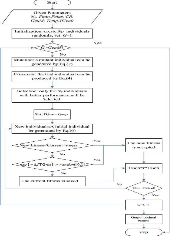
Flow chart of the HDE-SA
3.2. HDE-SA based procedures
3.2.1 Representation and initialization
Before initialization, the structure of the chromosome and mapping scheme should be determined. The chromosome has two parts: the first is the replenishment cycle of items, and the second is the delivery cycle of items. Therefore, the length of the chromosome is two times the number of items. Fig. 4 shows a decoded chromosome of six items.

Decoded chromosome (n=6).
The values of initial individual are randomly generated between 0 and 1, and then are mapped in practical solution (see Fig. 4) by decoding scheme. The formulation of decoding is as follow:
3.2.2 Illustrative example of the implementation of operations of HDE-SA
In this section, a simple example of a six-item problem is presented to better explain the implementation of HDE-SA.
- (1)
Mutation. Sequences of tth target vector, i.e., the tth individual is as follows:
0.8147 0.0975 0.1576 0.1419 0.6557 0.7577 0.7060 0.8235 0.4387 0.4898 0.2760 0.4984 Then, three integer numbers r1, r2, and r3 between 1 and Np, which are not the same as each other and are different from t, are generated randomly. Based on the position in the population, three individuals are selected as follows:
Sequences of popr1:
0.9134 0.9575 0.4854 0.7922 0.9340 0.6555 0.0462 0.9502 0.7952 0.7094 0.1626 0.5853 Sequences of popr2:
0.9058 0.2785 0.9706 0.4218 0.0357 0.7431 0.0318 0.6948 0.3816 0.4456 0.6797 0.9597 Sequences of popr3:
0.1270 0.5469 0.9572 0.9157 0.8491 0.3922 0.2769 0.3171 0.7655 0.6463 0.6551 0.3404
For Fmin= 0.2, Fmax= 0.8, the mutated vector popv is gained by Eq. (2) as follows:
1.5364 0.7428 0.4961 0.3970 0.2833 0.9362 −0.1499 1.2524 0.4880 0.5488 0.1823 1.0808 As the values of individuals before decoding is between 0 and 1, the values of gene (1), gene (7), gene (8), and gene (12) exceed the ranges. They are substituted by the numbers that are randomly generated from [0, 1]. Thus, the sequence of adjusted popv is:
0.8147 0.7428 0.4961 0.3970 0.2833 0.9362 0.7060 0.8235 0.4880 0.5488 0.1823 0.8308 - (2)
Crossover. At the same time, randn (t) is randomly generated and equal to 6.If CR= 0.6, the trial vector popu can be obtained by Eq. (4) as follows:
0.8147 0.0975 0.4961 0.3970 0.2833 0.7577 0.7060 0.8235 0.4880 0.5488 0.2760 0.8308 - (3)
Selection. Ultimately, after mutation and crossover operation, the next generation is formed by selecting between the trail vector and the corresponding target vector through comparing the total system cost according to Eq. (1). Then the trial vector popxG can be obtained according to Eq. (5) as follows:
0.8147 0.0975 0.4961 0.3970 0.2833 0.7577 0.7060 0.8235 0.4880 0.5488 0.2760 0.8308 - (4)
SA operation. After obtaining the trial vector popxG by HDE, a new vector popxuG is created according to Eq. (6) as follows:
0.0351 0.0042 0.0213 0.0171 0.0122 0.0326 0.0304 0.0354 0.0210 0.0236 0.0119 0.0357 Thereafter, we obtain the final vector popxG+1 by Eq. (7) as follows:
0.0351 0.0042 0.0213 0.0171 0.0122 0.0326 0.0304 0.0354 0.0210 0.0236 0.0119 0.0357 As the lower bound of two decision variables are set as 1s and the upper bound of two decision variables are set as 20s. We decode the chromosome according to Eq. (9) as follows:
2 1 1 1 1 2 2 2 1 1 1 2 For the given solution above, we can calculate the fitness, i.e., the TC by Eq. (1). When the maximum number of iteration is reached, output the optimal solution.
4. Numerical JRDs with trade credit and discussion
4.1. Different approaches selected for comparison
To test the performances of different approaches, the results of HDE-SA for the proposed JRD are compared with DE and GA for the following reasons:
- (a)
- (b)
4.2. Parameters setting analysis for HDE-SA
First of all, the parameters of the HDE-SA must be set. The HDE-SA has six control parameters, namely, NP, the population number; Fmin, Fmax, the mutation weighting factor; CR; Temp, the maximum temperature; TGen0, the termination temperature; and r, the ratio of the temperature drop. All of these parameters affect the speed and robustness of the search. The difficulty in using HDE-SA arises because the choice of these parameters depends on the empirical evidence and practical experience in most situations. However, many of these guidelines have good initial starting values that can be used directly. Wang, et.al [4] and Wang, Wang, and Liu [25] suggested that the guideline for the number of population is 2Nd ≤ Np ≤ 20Nd. In general, the larger NP is, the more robust the search is. Based on the recommendation of [4], the parameters are set as follows: CR=0.6; Fmin=0.2 and Fmax=0.8; GenM =150 when the number of items is 6 because it can converge to the optimum. TGen0 is set as 0.01. The parameters of GA are also set in accordance with the recommendation of Wang, et.al [4], i.e., Pc= 0.8 and Pm= 0.1.
To select proper parameters of HDE-SA for the proposed new JRD, Temp and r are confirmed by the following parameter-tuning test. The related data of the test example are shown in Table 1. The results are reported in Table 2.
| Item i | 1 | 2 | 3 | 4 | 5 | 6 |
|---|---|---|---|---|---|---|
| di | 600 | 1200 | 1800 | 2400 | 3000 | 3500 |
| siw | 30 | 33 | 36 | 39 | 42 | 45 |
| hiw | 4 | 5 | 6 | 8 | 10 | 12 |
| siR | 3 | 4 | 5 | 6 | 7 | 8 |
| hiR | 5 | 7 | 9 | 11 | 12 | 13 |
| c | 20 | 30 | 40 | 50 | 60 | 70 |
| p_i | 35 | 37 | 39 | 41 | 43 | 45 |
| i_p | 0.15 | 0.15 | 0.15 | 0.15 | 0.15 | 0.15 |
| I_e | 0.1 | 0.1 | 0.1 | 0.1 | 0.1 | 0.1 |
| M | 15/365 | 15/365 | 15/365 | 15/365 | 15/365 | 15/365 |
Data for the test example (Sw=100)
| Temp | r | Average TC | Min iteration | Max iteration | Avg iteration | CPU time (Seconds) |
|---|---|---|---|---|---|---|
| 500 | 0.9 | 11987.68 | 33 | 69 | 55.82 | 18.46 |
| 0.8 | 11987.68 | 38 | 65 | 54.74 | 8.88 | |
| 0.7 | 11987.68 | 37 | 69 | 55.96 | 5.4 | |
| 0.6 | 11987.68 | 44 | 65 | 56.02 | 4.19 | |
| 750 | 0.9 | 11987.68 | 37 | 67 | 55.56 | 16.9 |
| 0.8 | 11987.68 | 38 | 67 | 55.92 | 8.85 | |
| 0.7 | 11987.68 | 42 | 64 | 54.52 | 5.84 | |
| 0.6 | 11987.68 | 46 | 67 | 55.9 | 4.32 | |
| 1000 | 0.9 | 11987.68 | 36 | 71 | 56.18 | 17.55 |
| 0.8 | 11987.68 | 37 | 66 | 55.58 | 9.34 | |
| 0.7 | 11987.68 | 43 | 67 | 55.28 | 5.68 | |
| 0.6 | 11987.68 | 32 | 69 | 54.36 | 4.19 | |
Computational results under different Temp and r of HDE-SA (50 times, T=0.025)
Table 2 shows that the optimal solutions can always be found for Temp=1000 and r=0.6. Also, the average iteration of convergence and the CPU time are lower.
4.3. Numerical examples and results analysis.
4.3.1 Experiment 1: proposed JRD without trade credit
The proposed JRD is in fact a contrastive small-scale numeric example without trade credit based on the study of Cha et al. [5]. The data are shown in Table 3. In this case, the speed of obtaining the optimal solutions is not particularly emphasized.
| Item i | 1 | 2 | 3 | 4 | 5 | 6 |
|---|---|---|---|---|---|---|
| di | 10000 | 5000 | 3000 | 1000 | 600 | 200 |
| siw | 45 | 46 | 47 | 44 | 45 | 47 |
| hiw | 1 | 1 | 1 | 1 | 1 | 1 |
| siR | 5 | 5 | 5 | 5 | 5 | 5 |
| hiR | 1.5 | 1.5 | 1.5 | 1.5 | 1.5 | 1.5 |
Data for the example (Sw=200)
The result is shown in Table 4 and the convergence curves are presented in Fig. 5.
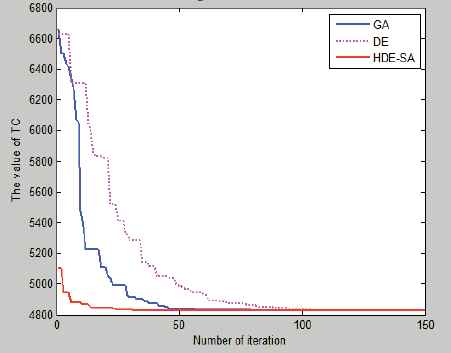
Convergence results for Experiment 1.
| Algorithm | T | ki | fi | TC |
|---|---|---|---|---|
| GA | 0.1881 | 1,1,1,2,2,4 | 4,3,2,3,2,2 | 4828.89 |
| DE | 0.1881 | 1,1,1,2,2,4 | 4,3,2,3,2,2 | 4828.89 |
| HDE-SA | 0.1881 | 1,1,1,2,2,4 | 4,3,2,3,2,2 | 4828.89 |
Comparison of three algorithms.
Thus, Temp=1000 and r=0.6 are regarded as suitable and are adopted in the following examples.
Then, we can draw the following conclusions:
- (a)
Both HDE-SA and DE can obtain the same optimal solution with GA. The optimal solution is the same as the finding of [5].
- (b)
The iteration of convergence of HDE-SA is better than that of DE and GA.
4.3.2 Experiment 2: proposed small-scale JRD with trade credit (n=6)
4.3.2.1 Results and analysis
After the proper parameters are confirmed, HDE-SA, DE, and GA are used to solve the proposed JRD with trade credit. The results are reported in Table 5.
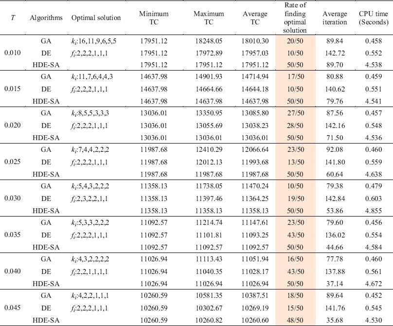
Comparison of HDE-SA, DE and GA for different T (50 times)
Table 5 shows that the proposed HDE-SA can always find an optimal solution, which indicates improved robustness. The average TC and average iteration of convergence with HDE-SA are also lower than those for DE and GA. Thus, the HDE-SA is an effective intelligent algorithm for the JRDs with trade credit.
4.3.2.2 Sensitivity analysis for Ie, Ip, and M
To further examine the effectiveness and stability of HDE-SA, we vary interest earned Ie, interest charged Ip, and credit period M from 30% to 30%, respectively. Computational results are presented in Tables 6–8.
| ΔIe | Average TC | Rate of finding the optimal solution | ||||
|---|---|---|---|---|---|---|
| GA | DE | HDE-SA | GA | DE | HDE-SA | |
| 30% | 12096.78 | 12003.54 | 11988.93 | 20/50 | 5/50 | 50/50 |
| 20% | 12085.64 | 11995.26 | 11988.51 | 17/50 | 14/50 | 50/50 |
| 10% | 12080.01 | 11991.45 | 11988.10 | 21/50 | 14/50 | 50/50 |
| −10% | 12069.60 | 11990.69 | 11987.26 | 23/50 | 20/50 | 50/50 |
| −20% | 12042.13 | 11989.11 | 11986.84 | 25/50 | 32/50 | 50/50 |
| −30% | 12036.63 | 11987.32 | 11986.42 | 21/50 | 36/50 | 50/50 |
Effects of interest earned Ie on total cost
| ΔIp | Average TC | Rate of finding the optimal solution | ||||
|---|---|---|---|---|---|---|
| GA | DE | HDE-SA | GA | DE | HDE-SA | |
| 30% | 12068.44 | 11993.54 | 11987.39 | 20/50 | 16/50 | 50/50 |
| 20% | 12093.59 | 11991.77 | 11987.48 | 13/50 | 21/50 | 50/50 |
| 10% | 12073.87 | 11993.09 | 11987.58 | 19/50 | 20/50 | 50/50 |
| −10% | 12061.93 | 11992.74 | 11987.77 | 19/50 | 24/50 | 50/50 |
| −20% | 12051.33 | 11990.70 | 11987.87 | 21/50 | 24/50 | 50/50 |
| −30% | 12076.09 | 11993.45 | 11987.97 | 21/50 | 22/50 | 50/50 |
Effects of interest charged Ip on total cost
| M | Average TC | Rate of finding the optimal solution | ||||
|---|---|---|---|---|---|---|
| GA | DE | HDE-SA | GA | DE | HDE-SA | |
| 5/365 | 11939.32 | 11938.82 | 11938.82 | 49/50 | 50/50 | 50/50 |
| 10/365 | 11998.05 | 11945.47 | 11943.70 | 22/50 | 39/50 | 50/50 |
| 20/365 | 12444.30 | 12394.62 | 12386.48 | 22/50 | 23/50 | 50/50 |
| 25/365 | 12431.14 | 12419.62 | 12402.62 | 25/50 | 9/50 | 50/50 |
Effects of credit period M on total cost
The results in Tables 6–8 show the effectiveness and stability of HDE-SA after running 50 times. Compared with GA and DE, HDE-SA can obtain a lower TC in all cases. All these contrastive results illustrate that HDE-SA is highly effective.
4.4 Experiment 3: larger-scale randomly generated JRDs with trade credit
In this section, the problem scale is extended to 10, 15, 20, 30, and 40 items, respectively, to further examine the performance of HDE-SA. The problems were generated randomly and each problem was run 50 times independently. The data are in Table 9. Results are reported in Table 10.
| di | siw | hiw | siR | hiR | c | pi |
|---|---|---|---|---|---|---|
| [500,5000] | [30,50] | [4,12] | [4,5] | [5,14] | [20,70] | [35,45] |
| S=100, i_p=0.15, I_e=0.1, M=15/365,T=0.025 | ||||||
Range of the parameter values
| n | Min TC | Max TC | Avg TC | Convergence Rate | Average iteration | CPU time (Seconds) | |
|---|---|---|---|---|---|---|---|
| 10 | GA | 19328.80 | 19509.52 | 19375.05 | 11/50 | 220.84 | 1.78 |
| DE | 19328.80 | 19441.35 | 19355.19 | 8/50 | 473.90 | 2.15 | |
| HDE-SA | 19328.80 | 19328.80 | 19328.80 | 50/50 | 210.54 | 16.98 | |
|
|
|||||||
| 15 | GA | 24523.82 | 24997.86 | 24747.58 | 1/50 | 623.88 | 2.86 |
| DE | 25255.14 | 25489.59 | 25424.29 | 1/50 | 722.30 | 3.36 | |
| HDE-SA | 24512.78 | 24512.78 | 24512.78 | 50/50 | 410.18 | 26.44 | |
|
|
|||||||
| 20 | GA | 30323.77 | 31254.48 | 30732.33 | 1/50 | 950.88 | 4.21 |
| DE | 32928.33 | 34417.45 | 33498.84 | 1/50 | 947.22 | 4.85 | |
| HDE-SA | 30107.39 | 30107.39 | 30107.39 | 50/50 | 667.82 | 38.68 | |
|
|
|||||||
| 30 | GA | 47094.83 | 49099.56 | 47909.97 | 1/50 | 1187.00 | 6.05 |
| DE | 57720.89 | 60172.09 | 58693.94 | 1/50 | 1135.25 | 6.91 | |
| HDE-SA | 44676.70 | 44726.04 | 44686.11 | 38/50 | 919.10 | 56.23 | |
|
|
|||||||
| 40 | GA | 74461.67 | 77498.00 | 75613.54 | 1/50 | 1429.45 | 8.19 |
| DE | 88413.20 | 92229.56 | 90816.91 | 1/50 | 1341.15 | 9.32 | |
| HDE-SA | 66402.55 | 66449.28 | 66416.26 | 18/50 | 1220.25 | 76.11 | |
Computational results for randomly problems (50times)
Table 10 shows that HDE-SA outperforms DE and GA in terms of accuracy and robustness. (a) The rate of finding an optimal solution with HDE-SA is higher than that for DE and GA, and the average iteration of convergence with HDE-SA is lower than that for DE and GA. Specifically, the convergence rate is 100% when n<20. In fact, the items that are jointly replenished are smaller than 20. (b) When n increases, the best TC and average TC obtained by HDE-SA is always better than that obtained by DE and GA. (c) Although HDESA is slower than DE and GA, the CPU time is acceptable for practical application.
Therefore, we can conclude that HDE-SA is an effective and robust algorithm to solve complex JRDs with trade credit in acceptable times.
4.5 Experiment 4: JRDs with trade credit considering resource constraint
In practice, JRPs have some constraints such as the limited transport equipment capacity and budget. Moon and Cha [5] compared their GA with the proposed heuristic to test the ability of GA to solve the JRD with some constraints. Qu [10] solve the JRD considering the grouping constraint during the transportation process.
Some heuristics cannot work as efficiently as possible in handling many constraints at the same time. In this study, we consider JRD with trade credit, so the budget constraint is not further discussed. Therefore, our model is extended by considering two types of transportation restrictions. One is the joint replenishment constraint, and the other is the outbound delivery constraint. The former can be represented as follows:
So, we can know that
The way to solve the JRD with constraint is similar to the procedures in Section 3.2. The difference is the setting of the upper bounds of Ki. For the case of no resource restriction, the upper bounds of ki are directly set to 20s according to the suggestion of Qu et al. [10].
When the constraint is considered, the upper bounds of ki is
By adding a resource constraint to Experiment 3(we assume BW = 25,000 and all bi = 6.25 and BiR=2000), the following results are obtained, in comparison with the case without the resource constraint. In case of T=0.025, the detailed solution obtained by HDE-SA is shown in Table 11. The problems were generated randomly and each problem was run 50 times independently and the results are reported in Table 12. For other parameters of T, the same conclusion is obtained.
| n | ki | fi | TC | |
|---|---|---|---|---|
| 10 | No.Restriction | 2,4,3,3,5,2,2,2,6,2 | 1,2,1,1,3,1,1,1,1,1 | 20126.90 |
| Resource restriction | 1,3,3,2,5,1,1,1,6,1 | 1,1,1,1,3,1,1,1,1,1 | 24244.18 |
Results of an illustrative example of the proposed JRDs by HDE-SA (n=10)
| n | Algorithms | Minimum TC | Maximum TC | Average TC | CPU time (Seconds) | |
|---|---|---|---|---|---|---|
| 10 | GA | No. constraint | 17779.50 | 18080.53 | 17867.83 | 1.23 |
| Resource constraint | 18817.45 | 18817.45 | 18817.45 | 1.24 | ||
|
|
||||||
| DE | No. constraint | 17779.50 | 17913.04 | 17828.16 | 1.89 | |
| Resource constraint | 18817.45 | 18817.45 | 18817.45 | 2.78 | ||
|
|
||||||
| HDE-SA | No. constraint | 17779.50 | 17779.50 | 17779.50 | 15.92 | |
| Resource constraint | 18817.45 | 18817.45 | 18817.45 | 15.79 | ||
|
|
||||||
| 15 | GA | No. constraint | 22619.08 | 23078.22 | 22715.71 | 2.06 |
| Resource constraint | 25022.91 | 25188.02 | 25067.81 | 2.02 | ||
|
|
||||||
| DE | No. constraint | 23044.70 | 23722.14 | 23357.98 | 3.12 | |
| Resource constraint | 25048.06 | 25311.45 | 25174.74 | 3.08 | ||
|
|
||||||
| HDE-SA | No. constraint | 22619.08 | 22619.08 | 22619.08 | 26.34 | |
| Resource constraint | 25022.91 | 25029.49 | 25025.22 | 26.25 | ||
|
|
||||||
| 20 | GA | No. constraint | 32048.16 | 32466.04 | 32273.10 | 3.11 |
| Resource constraint | 33620.02 | 33696.91 | 33628.46 | 3.11 | ||
|
|
||||||
| DE | No. constraint | 34757.80 | 36249.77 | 35496.85 | 4.94 | |
| Resource constraint | 36714.64 | 38550.48 | 37705.02 | 3.56 | ||
|
|
||||||
| HDE-SA | No. constraint | 31951.07 | 31987.70 | 31954.65 | 41.89 | |
| Resource constraint | 33620.02 | 33620.02 | 33620.02 | 40.59 | ||
|
|
||||||
| 30 | GA | No. constraint | 50653.42 | 52354.12 | 51625.34 | 6.71 |
| Resource constraint | 54389.23 | 54752.90 | 54598.67 | 6.66 | ||
|
|
||||||
| DE | No. constraint | 60602.61 | 64187.84 | 62598.15 | 10.32 | |
| Resource constraint | 68469.70 | 71749.43 | 70200.91 | 5.08 | ||
|
|
||||||
| HDE-SA | No. constraint | 48344.02 | 48360.48 | 48346.51 | 85.60 | |
| Resource constraint | 54386.89 | 54389.23 | 54387.71 | 84.18 | ||
|
|
||||||
| 40 | GA | No. constraint | 67353.20 | 69137.23 | 68021.20 | 8.66 |
| Resource constraint | 68160.58 | 69784.88 | 68921.03 | 8.73 | ||
|
|
||||||
| DE | No. constraint | 79699.58 | 82364.81 | 81038.44 | 13.57 | |
| Resource constraint | 86127.13 | 89232.20 | 87857.00 | 5.71 | ||
|
|
||||||
| HDE-SA | No. constraint | 61094.19 | 61171.27 | 61118.39 | 110.17 | |
| Resource constraint | 67231.26 | 67502.26 | 67324.28 | 109.90 | ||
Results of JRDs with/without the resource constraint by different algorithms
Table 12 also shows the following conclusions: (a) The average TC is higher when the resource restriction is considered. (b) HDE-SA outperforms DE and GA in terms of average TC. (c) HDE-SA is slower than DE and GA, but the CPU time is still acceptable for the practical viewpoint.
5. Conclusions and future research
This study is an interdisciplinary study on the inventory and delivery model and intelligent optimization algorithm. We propose a useful and new joint multi-item replenishment and delivery model considering trade credit. The objective is to determine the optimal replenishment and delivery schedule while minimizing the total cost. To our knowledge, this study represents the first time that the joint multi-item replenishment and delivery schedule problem is proposed by considering the trade credit. This study extends the research on traditional JRDs with relatively high theoretical significance and practical value.
To resolve this NP-hard problem, an effective HDESA is designed by integrating the advantages of DE and SA. The performance of the HDE-SA is verified by different scales of JRDs with trade credit. Numerical JRD examples illustrate the effective and robust performance of HDE-SA. Compared with other popular evolutionary algorithms, HDE-SA can always acquire slightly lower total costs under different cases. Moreover, the convergence rate of HDE-SA is higher than that of DE and GA. Moreover, the HDE-SA can be easily applied to these types of JRDs with resource constraints to find satisfactory solutions. Therefore, HDE-SA is a strong candidate for solving JRDS under trade credit because of the distinct advantages of robustness, easy implementation, and quick convergence.
In future research, there are possible improvements of this study to be further discussed. Other intelligent algorithms, such as genetic-simulated annealing algorithm and fruit fly optimization algorithm [26–27], show good performance in solving complex optimization problems. We intend to design hybrid algorithms by taking advantage of the aforementioned algorithms in handling more complex JRDs. Moreover, decision makers often have to face vague or imprecise operational conditions in reality [28–29]. It is interesting to consider stochastic or fuzzy demand for handling more practical JRDs under uncertain supply chain environment in the network economic era [30–32].
Acknowledgements
The authors are grateful for the constructive comments of editors and referees. This research is partially supported by Humanities and Social Sciences Foundation of Chinese Ministry of Education (No. 15YJA630095).
References
Cite this article
TY  - JOUR
AU  - Yu-Rong Zeng
AU  - Lu Peng
AU  - Jinlong Zhang
AU  - Lin Wang
PY  - 2016
DA  - 2016/12/01
TI  - An Effective Hybrid Differential Evolution Algorithm Incorporating Simulated Annealing for Joint Replenishment and Delivery Problem with Trade Credit
JO  - International Journal of Computational Intelligence Systems
SP  - 1001
EP  - 1015
VL  - 9
IS  - 6
SN  - 1875-6883
UR  - https://doi.org/10.1080/18756891.2016.1256567
DO  - 10.1080/18756891.2016.1256567
ID  - Zeng2016
ER  -