
Efficient Greedy Randomized Adaptive Search Procedure for the Generalized Regenerator Location Problem
- DOI
- 10.1080/18756891.2016.1256568How to use a DOI?
- Keywords
- GRASP; regenerator; telecommunications; metaheuristic; generalized regenerator location problem
- Abstract
Over the years, there has been an evolution in the manner in which we perform traditional tasks. Nowadays, almost every simple action that we can think about involves the connection among two or more devices. It is desirable to have a high quality connection among devices, by using electronic or optical signals. Therefore, it is really important to have a reliable connection among terminals in the network. However, the transmission of the signal deteriorates when increasing the distance among devices. There exists a special piece of equipment that we can deploy in a network, called regenerator, which is able to restore the signal transmitted through it, in order to maintain its quality. Deploying a regenerator in a network is generally expensive, so it is important to minimize the number of regenerators used. In this paper we focus on the Generalized Regenerator Location Problem (GRLP), which tries to find the minimum number of regenerators that must be deployed in a network in order to have a reliable communication without loss of quality. We present a GRASP metaheuristic in order to find good solutions for the GRLP. The results obtained by the proposal are compared with the best previous methods for this problem. We conduct an extensive computational experience with 60 large and challenging instances, emerging the proposed method as the best performing one. This fact is finally supported by non-parametric statistical tests.
- Copyright
- © 2016. the authors. Co-published by Atlantis Press and Taylor & Francis
- Open Access
- This is an open access article under the CC BY-NC license (http://creativecommons.org/licences/by-nc/4.0/).
1. Introduction
Last years society has become more and more connection dependent, in such a way that nowadays it is hard to think in accomplishing a common task without using some kind of connection among two or more devices. In most cases, we need a reliable connection to transmit information in the form of electronic or optical signals. For that reason, the correct transmission of these signals has become an essential part in our lives. The transmission of a signal between two points is not usually direct, because the two endpoints of the communication are usually rather separated. For that reason, the signal travels through a dense network of electronic devices, creating a path between the two endpoints. However, the strength of the signal is usually deteriorated as it gets farther from the source, mainly due to attenuation. Then, in order to maintain the quality of the signal, it is necessary to regenerate it periodically by using a special type of electronic device in the network called regenerator 1. These pieces of equipment are usually expensive, so we need to deploy the lowest number of regenerators in order to reduce the cost of the signal transmission.
In general, a network is usually modeled with a graph G = (V, E), where the set of nodes V represents electronic devices and the set of edges E represents the link connections between electronic devices. Each edge (u, v) ∈ E presents a length duv > 0 which corresponds to the distance between nodes u and v. The set of nodes is divided into two subsets. The first one, S ⊆ V, contains the candidate locations to deploy a regenerator; while the second one, T ⊆ V, represents the set of terminal nodes that must communicate with each other. Notice that T and S are disjoint sets (i.e., T ∩ S = ∅ and T ∪ S = V).
Each terminal node must be able to send signals to the other terminal nodes throughout a path without exceeding a maximum given distance, dmax > 0, in order to avoid the deterioration of the signal. Specifically, the path, P, between an origin terminal to and a destination terminal td through the network G is defined as the set of nodes that should be traversed in order to reach td starting from to:
If d(Pto,td) ⩽ dmax the signal can travel directly from to to td without the necessity of regenerating the signal. Therefore, the terminals of a network are fully connected if the shortest path between each pair of terminals nodes presents a distance lower than dmax. In mathematical terms,
Otherwise, in order to assure a proper communication among terminal nodes, regenerators must be deployed in one or more nodes in the paths where d(Pto,td) > dmax. These regenerators are able to restore the signal in the node where they are installed, in such a way that the distance traveled by the signal starts again from zero after reaching a regenerator in the path. This behavior allows the signal to be transmitted for longer distances. Therefore, the distance between two terminal nodes through a path that contains one or more regenerators is evaluated as:
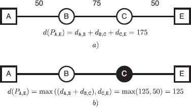
Evaluation of a path distance when (a) no regenerators are deployed and (b) when a regenerator is deployed in node C.
This optimization problem has been identified in the related literature as the Generalized Regenerator Location Problem (GRLP). The objective function of this problem is then to find the subset of regenerators R ⊆ S with the minimum cardinality that allows the communication among all terminal nodes without exceeding the maximum distance. In mathematical terms:
Regenerator placement problems have been widely studied in the recent years due to its importance in the area of telecommunications. Yetginer and Karasan 2 present one of the first works in the context of traffic engineering with restoration, while Gouveia et al. 3 address a multi-protocol label switching over wave division multiplexing network design. In Chen et al. 4,5,6 several methods for the Regenerator Location Problem (RLP) are presented. This optimization problem is a variant for the GRLP where S = T = V (there are not distinctions between terminal nodes and candidate locations). More recently, Duarte et al. 6 proposed a GRASP procedure and a Biased Random Key Genetic algorithm. A strategic oscillation procedure is presented for the Maximum Leaf Spanning Tree Problem 7, which presents an isomorphism with the RLP. Finally, Chen et al. 8 formally defines the GRLP as a generalization of the RLP. This problem was proved to be NP-hard by Chen et al. 5 and Flammini et al. 9. In spite of the importance of this problem in the optical network design and telecommunications, GRLP has been barely ignored from the heuristic point of view. Specifically, we have only found one work 10 focused in the GRLP, where authors propose a branch-and-cut algorithm as well as two heuristics for solving the GRLP.
In this paper we propose an algorithm based on the Greedy Randomized Adaptive Search Procedure (GRASP) metaheuristic 11. Specifically, we introduce two constructive procedures and a local search method within the GRASP methodology. Additionally, we propose two different enhancement for reducing the computing time required by the local search method, together with a procedure which removes unnecessary regenerators.
The rest of the paper is organized as follows: Section 2 describes a graph transformation algorithm that simplifies the resolution of the GRLP. Section 3 describes the algorithm proposal. We select the best GRASP variant and then compare it with the current state of the art in Section 4. Finally, main conclusions are presented in Section 5.
2. Communication graph
The communication graph is introduced as a graph transformation procedure to convert the original network into a simpler model 10. Specifically, considering the original graph G = (V, E), with V = S ∪ T, the first step consists of removing all edges with length larger than dmax. These edges are useless (from a communication point of view) in the network since it is not possible to send the information through them. In other words, the signal would not have not enough quality to be processed at the destination because of the distance.
For all non-adjacent pairs of nodes, the next step of this procedure consists of adding an artificial edge between them. Its associated length is equal to the length of the corresponding shortest path. As it was aforementioned, artificial edges with length larger than dmax are eliminated since it is not possible to send information through them.
Artificial edges model the situation where an origin sends information to a destination through several intermediate nodes but the total traveled distance is lower than or equal to the maximum allowed one. Notice that it is equivalent to send the information through the shortest path or, alternatively, through the artificial added edge. At this step, we can discard the distance information, resulting in an unweighted graph, M = (V, E′).
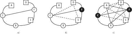
Figure 2.a shows an example of an original graph G, where terminal nodes are represented within a square (A, E, and F) and those which can hold a regenerator with a circle (B, C, and D). The numbers in the edges indicates the distance between the linked nodes. Let us suppose that the maximum distance that a signal can travel is set to 150. Then, the communication graph is constructed by firstly removing those edges whose distance is larger than the maximum distance. In this example only edge (A, D) is removed (see Figure 2.b). The next step computes the shortest path between each pair of nodes. For the sake of simplicity we only report information about shortest paths responsible of adding new artificial edges (i.e., the corresponding length is lower than or equal to 150). In particular, the procedure adds the following edges:
- •
Edge (A, C), with path: {dA,B, dB,C} = 50 + 75 = 125.
- •
Edge (A, D), with path: {dA,B, dB,D} = 50 + 100 = 150.
- •
Edge (B, E), with path: {dB,C, dC,E} = 50 + 75 = 125.
- •
Edge (B, F), with path: {dB,D, dD,F} = 100 + 50 = 150.
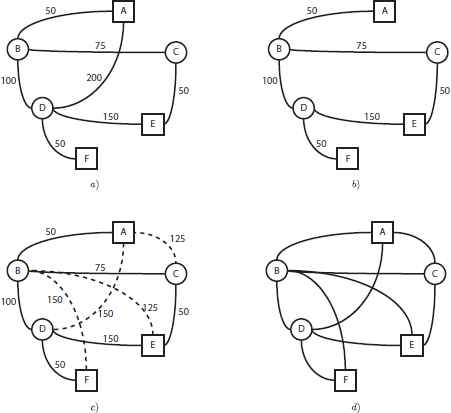
Construction of the communication graph.
Figure 2.c shows the resulting intermediate communication graph. Finally, in Figure 2.d we show the final communication graph where the length information is discarded.
The communication graph is particularly useful when evaluating the effect of including a new regenerator in the network. In particular, if a node s ∈ S holds a regenerator, the signal can be restored and, therefore, transmitted to all nodes directly connected to s (i.e., the set of adjacent nodes, N(s)= {v ∈ V : (s, v) ∈ E}). This property is reflected in the communication graph as the inclusion of several new artificial edges between each pair of adjacent nodes to s. Notice that the actual added artificial edges are those not previously present in the communication graph.
Let t1, t2 ∈ T be two non-adjacent terminal nodes in the communication graph and let s ∈ S ∩ N(t1) ∩ N(t2) be a candidate node to hold a regenerator adjacent to both, t1 and t2 (see Figure 3.a). In this situation, terminal t1 can share information with s. Similarly, s can share information with t2. However, t1 cannot share information with t2 unless we place a regenerator in s to restore the quality of the signal. Therefore, the inclusion of a regenerator in s allows the communication between t1 and t2, which is equivalent to include an artificial edge between t1 and t2 in the communication graph. We illustrate this situation in Figure 3.b by adding a new edge represented with a dotted line.
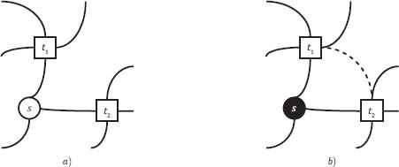
Construction of the communication graph.
As a result, given a graph G = (V, E), and its associated communication graph, M = (V, E′), a node v ∈ V can send a signal to another one u ∈ V, (without loss of quality) if and only if there exist an edge (u, v) ∈ E′. The objective of the GRLP is to connect all terminal nodes among them. Therefore, a solution R, (i.e., set of included regenerators) is feasible if the associated communication graph has an edge between each pair of terminal nodes. Let us illustrate this situation by considering the example depicted in Figure 2.d. The solution derived from this communication graph (i.e. R = ∅) is not feasible. More precisely, not all the terminal nodes are connected, see {(A, E), (A, F), (E, F)}. In order to obtain a feasible solution, it is necessary to insert some regenerators in the communication graph. For example, if we deploy a regenerator in vertex C (which implies R = {C}) all nodes adjacent to C, (i.e., vertices A, B, and E), become connected. Considering the set of terminal nodes, the inclusion of a regenerator in C only adds the edge (A, E). As it is shown in Figure 4.a, this solution is not feasible since not all terminal nodes are directly connected (see for instance A and F). If we add a new additional regenerator in node B, the solution becomes feasible since all terminal nodes are able to share information (i.e., there is an edge between each pair of terminals). Therefore, the solution is R = {C, B}, whose objective function value is |R| = 2, which means that we have deployed two regenerators to connect all terminals in T. Notice that this is not the optimal solution since we can connect all terminal nodes by deploying a single regenerator in node B.
Communication graph resulting from the insertion of a regenerator in (a) node C and (b) in node B in the graph depicted in Figure 2.d. New edges are represented with dotted lines.
Therefore, the objective of the GRLP is based on connecting those terminal nodes which are not directly connected in the corresponding communication graph M. The connections are created by including new regenerators in the graph which generate new edges between pairs of terminal nodes. The set of non-directly connected terminal nodes in a given communication graph is denoted as NDC (M, R). For example, analyzing the communication graph depicted in Figure 2.d, NDC (M, R)= {(A, E), (A, F), (E, F)}. The deployment of a regenerator in node C as depicted in Figure 4.a eliminates the pair (A, E) from the NDC set. Finally, the regenerator deployed in node B removes pairs (A, F) and (E, F) from the NDC set, resulting in an empty NDC set and, therefore, in a feasible solution (see Figure 4.b).
3. Greedy randomized adaptive search procedure
In this paper we propose an algorithm based on the Greedy Randomized Adaptive Search Procedure (GRASP) metaheuristic. GRASP was developed by12 in the late 80s, but it was not formally introduced until 1994 11. Recent surveys on the methodology have been presented 13,14. The main idea behind GRASP methodology is to iteratively and stochastically sample greedy solutions, and then improve them to reach a local optimum. This stages are repeated until a termination criterion is met. In this paper we propose two constructive procedures and an efficient method. The GRASP algorithm selects a constructive method to generate initial solutions during a preset number of iterations. For each generated solution, the algorithm uses the improvement method proposed to obtain a local optimum. Finally, the algorithm stores the best solution found during the exploration. This metaheuristic has been successfully applied in several recent NP-hard problems15,16.
3.1. Constructive procedures
Starting from scratch, a classical GRASP constructive procedure iteratively builds a solution adding an element at each step. The set of eligible elements are usually denoted as Candidate List (CL). In the context of the GRLP, all the nodes in S are candidates to hold a regenerator. Therefore, at the beginning of the process CL = S. Then, each node v ∈ CL is evaluated with a greedy function. In this paper, we introduce a greedy function, named g1, which is defined as the number of terminal nodes connected to v. The rationale behind this idea is that regenerators should be deployed in those nodes which are connected to the maximum number of terminal nodes, creating several artificial edges between them. In mathematical terms:

Algorithm C1.
The procedure starts by creating the CL with the nodes that can host a regenerator (step 3). Then, in each step, the RCL is constructed as described above (steps 5–8). In step 9, a node is selected at random from the RCL, and added to the solution (step 10). Finally, the communication graph is updated, by adding new edges between each pair of adjacent nodes to v (step 11). The CL is also updated by removing v (step 12). The procedure continues adding new nodes to the solution until the NDC associated to the communication graph becomes empty (steps 4–13). In this case, the procedure returns the constructed solution R.
We propose a second constructive procedure (C2) whose main difference with respect to the previous one is the greedy function used to evaluate the nodes in the CL. In this case, the greedy function g2 is intended to promote those nodes which create the maximum number of edges between non-directly connected terminal nodes when holding a regenerator. More formally,
We do not include a pseudocode for the second constructive procedure since it is equivalent to the one presented in Algorithm 5, but using g2 instead of g1 in steps 5, 6, and 8.
The solutions constructed using the proposed procedures may contain some nodes which do not need to actually hold a regenerator in order to have a feasible solution. Let us illustrate this situation with the example depicted in Figure 3.b. The deployment of a genenerator in node C creates an edge between A and E, while the regenerator in B includes the same edge (A, E) and other additional edges between terminal nodes {(A, F), (E, F)}. Therefore, we can remove node C from the solution, keeping it feasible, and producing a better solution with only one regenerator deployed in node B.
Given a communication graph M and a solution R, we propose a procedure clean(M, R) which iterates over every node v ∈ R. For each node, the procedure checks whether the solution remains feasible when removing the regenerator or not. In case the solution remains feasible, the regenerator is definitively removed from the solution. Otherwise, it is included again on it. The clean procedure is performed for each constructed solution, in order to remove redundant regenerators.
3.2. Improvement method
The second phase of a GRASP algorithm consists of improving the constructed solution until reaching a local optimum. Before proposing a local search procedure, it is necessary to define which moves are allowed during the search. In the context of GRLP, we propose two different and complimentary moves: insert and remove. The insert move consists of adding a new node to the solution, deploying a regenerator in it, while the remove one consists of deleting a node from the current solution, removing its corresponding regenerator.
The local search proposed in this work (LS) tries to reduce the number of regenerators contained in a given solution by performing an exhaustive search. Specifically, in each iteration, the method tries to remove two regenerators, deploying only a new one. If the resulting solution is still feasible, the number of regenerators would have been reduced in one unit, improving the original solution. Figure 6 presents the pseudocode of the proposed method.
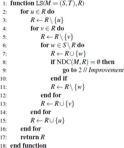
Algorithm LS.
The local search method iterates over each pair of regenerators already deployed in the solution (steps 2–16 and 4–14, respectively). In each iteration, two regenerators are removed from the solution R (steps 3 and 5). Then, the procedure iterates over the list of possible regenerators (steps 6–12). For each potential node to hold a regenerator, LS inserts it in the solution (step 7). If the new solution is feasible (step 8), i.e., all terminal nodes are connected, then an improved solution has been found, restarting the search (step 9). Otherwise, the method restores the solution by removing the included regenerator (step 11), and including the previously removed ones (steps 13 and 15). The procedure ends when no improvement is found, returning the best solution found in the search.
The exhaustive nature of the proposed local search method makes it computationally intensive in terms of CPU time. Therefore, we propose two different enhancements which make the search more efficient without loss of quality. The first enhancement, denoted as LSpred, is intended to avoid performing those moves which leads to unfeasible solutions. Before inserting the next node in the solution (step 7), it is possible to predict whether the insertion will result in a feasible solution or not. The insertion of a node v produces a feasible solution if and only if each node which appears in the NDC is adjacent to v. The rationale behind this idea is that deploying a regenerator in v will generate an edge between each pair of adjacent vertices to it and, therefore, the corresponding pair in the NDC will be removed. In other words, if the regenerator is able to connect all pairs in the NDC, the solution remains feasible. More formally, given a communication graph M and an unfeasible solution R, the inclusion of a regenerator in v makes R feasible if ∀ u ∈ NDC (M, R) ∃ (v, u) ∈ E′. In order to include this enhancement, the insertion of a new node in the solution (step 7 of Algorithm 6) is modified by considering only those ones that result in a feasible solution.
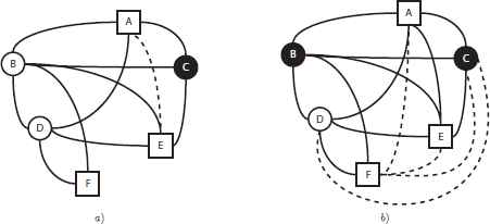
The second enhancement introduced in this paper, named LSstack, is intended to increase the efficiency of the search by reducing the computing time of updating the communication graph after removing a regenerator (see steps 3 and 5 of Algorithm 6). In order to do that, we need to determine the regenerator responsible of including new artificial edges in the communication graph. It is worth mentioning that these edges depends on the order in which regenerators were included in the solution. Let us illustrate this fact by considering the example depicted in Figure 7. Specifically, we show in Figure 7.a the original communication graph. If we firstly deploy a regenerator in F then three new edges are created, (C, D), (C, E), and (D, E). See Figure 7.b, where the new added edges are represented with dotted lines. However, if the first regenerator has been deployed in C, and then we deploy a regenerator in F (Figure 7.c), then three additional edges are created, (A, D), (B, D) and (A, E).
Result of deploying a regenerator in F in different order: (b) the first regenerator and (c) second one. New edges created by F are represented with dotted lines.
We can conclude that the edges created by the insertion of a regenerator in a solution not only depends on the node itself, but also on the previously introduced ones. Therefore, in a straightforward implementation, if we eliminate a regenerator, we must reconstruct the communication graph from scratch, since it is not possible to isolate the effect of removing a single regenerator from the solution. However, if we consider the order in which the regenerators were introduced in the solution, we can significantly reduce the number of operations needed to update the communication graph.
Say for instance that we want to remove the regenerator in v. In order to do that, we firstly eliminate all regenerators that were added after it. Then, we actually remove v, and finally insert again, in the same order, the removed regenerators (those originally inserted after v). Following these three steps, we can assure that those edges created by the regenerators added after v, which were originally created due the previous deployment of a regenerator in v, have been effectively removed from the communication graph.
Figure 8 shows an example of the removal of a regenerator. Let us assume that this solution was constructed by firstly deploying a regenerator in C and then in F. As it can be easily tested, it is a feasible solution with two regenerators (black colored), since all terminals (represented with a square) are connected. The first step to remove C consist of eliminating those regenerators that were inserted after it. Since F was inserted after C, then we need to remove it from the communication graph, along with the associated edges (represented with dotted line) that were created due to its insertion (see Figure 8, 1 - Remove F). In the next step (Figure 8, 2 - Remove C), renegerator in node C and its associated edges (represented with dotted line) are removed from the graph. Finally, we need to insert again those regenerators that were removed in the first step. In this case, we only need to deploy a regenerator in F, creating the edges (C, D), (C, E) and (D, E) during the process.
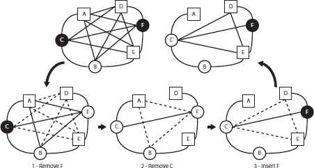
Removal of the regenerator deployed in C considering the order of insertion [C, F].
Considering the aforementioned situation, the number of operations required to update the communication graph depends on the order in which it was inserted. In particular, the sooner the regenerator was deployed, the larger the complexity of the corresponding update when removing it. However if we store the regenerators in a specific data structure that keeps information about the time in which they were specifically included in the solution, we could reduce the computing time employed in updating the communication graph. This data structure is usually known as stack, where the last element included in it (operation called push) is extracted in the fist place (operation called pop), following the Last-In First-Out (LIFO) strategy. In the context of the GRLP, if we want to remove a regenerator v from the solution, it is only needed to iteratively pop elements from the stack until removing v, and then push them again (excluding v) in to the stack. Then, all edges created by regenerators included before v does not require any update operation, saving a considerable computing time.
The local search that incorporates this enhancement is called LSstack. It traverses the regenerators to be removed from the solution by following the order of the stack. Specifically, it starts by removing regenerators close to the top of the stack (resulting in faster removals), while the regenerators that are at the bottom of the stack and, therefore, those which requires more computing time, are the last ones to be explored. In the next section we will experimentally evaluate the performance of the proposed enhancements.
4. Computational experiments
This Section presents the computational experiments performed to test the quality of the proposed algorithms for the GRLP. They were implemented in Java SE 8 and the experiments were conducted on an Intel Core i5 2410M CPU (2.30 GHz) and 8GB RAM. Three different sets of instances where introduce in Chen et al. 10. However, the exact procedure propose in the same paper finds the optimal solution in some of them in less than an hour. Therefore, we exclude these instances since they are not an actual challenge for heuristic methods. We then consider the subset of 60 instances where the optimum is unknown. Each one is parametrized by the number of nodes (n) and the percentage of terminal nodes (p). The benchmark presents 10 instances for each value of n and p in the range n ∈ {400, 500} and p ∈ {0.25, 0.50, 0.75}.
The experiments are divided into two different parts: preliminary and final experimentation. The former is intended to (i) select the best variant among our proposed methods and (ii) evaluate the influence of each proposed strategy over the final performance. The objective of the latter is to conduct a comparison between our best algorithm with the best one found in the literature 10.
4.1. Preliminary experimentation
We have selected a subset of 18 representative instances (3 from each value of n and p) for the preliminary experimentation in order to avoid over-training. For each experiment, we report the following statistics: average number of regenerators deployed, Avg.; computing time measured in seconds, Time (s); average percentage deviation with respect to the best solution found in the experiment, Dev (%); and the number of times that a given procedure matches the best solution found in the preliminary experimentation, # Best.
The first experiment is designed to select the best constructive method by comparing C1 and C2 (see Section 3.1). We consider different values for the α parameter to evaluate how it influences the performance of each variant. Specifically, we set α = {0.25n, 0.50n, 0.75n}, where n is the number of nodes in the instance. The variation in the α parameter allows us to study the influence of the balance between diversification and intensification in the constructive procedure 17. As it is customary in GRASP, we execute 100 independent times each constructive method, reporting the best solution found. Table 1 presents the results obtained by the aforementioned variants. These results show that C2 is slower than C1, but obtaining considerably better results in terms of objective function value, average deviation and number of best solutions found. Specifically, C2 with α = 0.75 is the best constructive method found, with a deviation of 0.12% with respect to the best solution.
| C1 | C2 | |||||
|---|---|---|---|---|---|---|
| α | 0.25 | 0.50 | 0.75 | 0.25 | 0.50 | 0.75 |
| Avg. | 31.38 | 62.82 | 103.69 | 22.42 | 19.36 | 17.18 |
| Time (s) | 51.21 | 78.58 | 79.66 | 2769.23 | 2182.54 | 2031.72 |
| Dev (%) | 0.98 | 3.22 | 6.63 | 0.48 | 0.27 | 0.12 |
| # Best | 0 | 0 | 0 | 0 | 1 | 7 |
Comparison of constructive methods when considering different values for α
It is worth mentioning that the computing time is unexpectedly large for a constructive procedure. In order to reduce this time, we decrease the number of independent executions, from 100 to 5. However, this strategy produces, as a side effect, lower quality solutions. With the objective of compensate this loss of quality, we include the clean method proposed in Section 3.1, whose goal is to eliminate the unnecessary regenerators after constructing a solution. Table 2 presents the results obtained by the constructive coupled with the clean procedure. These results show that the impact of this strategy has different effects in C1 and C2. Specifically, the computing time of variants based on C1 is increased. However, the solutions found present considerably larger quality. In the case of C2, the reduction in the CPU time is remarkable, while maintaining or even increasing the quality of the constructed solutions. Analyzing these results, C2 with α = 0.75 emerges as the best method. We then select it for the rest of the experimentation.
| C1 | C2 | |||||
|---|---|---|---|---|---|---|
| α | 0.25 | 0.50 | 0.75 | 0.25 | 0.50 | 0.75 |
| Avg. | 19.73 | 19.13 | 19.13 | 19.62 | 18.76 | 17.31 |
| Time (s) | 268.54 | 534.09 | 570.92 | 805.17 | 661.46 | 556.08 |
| Dev (%) | 0.31 | 0.27 | 0.26 | 0.30 | 0.24 | 0.14 |
| # Best | 0 | 2 | 2 | 0 | 1 | 1 |
Comparison of constructive methods when applying the clean procedure after each construction
The next experiment is intended to analyze the influence of the proposed enhancements for the local search method described in Section 3.2. In particular, we evaluate the behavior of each enhancement isolated and then combine them in the same local search variant. Figure 9 shows the computing time needed to execute the local search method with each corresponding enhancement. Specifically, LS refers to the local search with no enhancements, LSpred includes the first enhancement proposed, and LSstack considers the second enhancement. Finally, LScomb corresponds to the local search method which considers both enhancements at the same time.
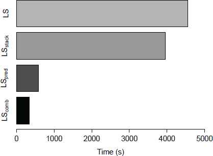
Performance comparison of the proposed enhancements for the local search procedure.
Given two algorithms whose computing time is time1 and time2, respectively, the speedup is defined as S = time1/time2. If S > 1 then we can conclude that the first compared algorithm is faster than the second one. Obviously, if S < 1, the conclusion is just the opposite. The results depicted in Figure 9 show that the use of a stack (LSstack) reduces the computing time in 500 seconds approximately, achieving a speedup of 1.14, which means that this variant is 14% faster than the basic approach. LSpred is able to reduce the computing time in 3900 seconds, obtaining a speedup of 7.70 with respect to the basic approach. Finally, the combination of both enhancements, LScomb, is able to obtain a speedup of 13.13 with respect to LS. Therefore, we select this variant for the final version of the algorithm.
4.2. Final experimentation
The final experiment is intended to evaluate the performance of our best proposal compared with the best methods found in the state of the art 10. In particular, our best proposal is a GRASP algorithm which is configured with C2 (α = 0.75) coupled with the clean method and the local search with the combined enhancements, LScomb, as the improving strategy. In order to have a fair comparison, our proposal has been executed for the same computing time as the best previous methods for the GRLP, i.e., the two heuristics (GH1 and GH2) presented in 10. For the sake of completeness, we also include the results of the branch-and-cut method (B&C) to have an estimation about the quality of the heuristic solutions. Specifically, we include the upper bound (UB) and lower bound (LB) that establishes the interval in which the optimal solution is located. This method has been executed for a maximum computing time of one hour.
Table 3 reports, for each size n and percentage of terminal nodes p, the results averaged over 10 instances. For each method (column), we show the average number of deployed regenerators, Avg., and the CPU time in seconds, Time (s). The last row shows the average results over the whole set of 60 instances.
| B&C | GH1 | GH2 | GRASP | ||||||
|---|---|---|---|---|---|---|---|---|---|
| n | p(%) | UB | LB | Avg. | Time (s) | Avg. | Time (s) | Avg. | Time (s) |
| 400 | 25 | 21.90 | 13.30 | 22.40 | 7.40 | 22.40 | 8.90 | 20.90 | 6.85 |
| 50 | 19.60 | 11.10 | 19.80 | 20.30 | 20.00 | 18.80 | 18.30 | 19.53 | |
| 75 | 14.40 | 9.50 | 14.70 | 4.70 | 14.40 | 6.00 | 13.90 | 4.62 | |
| 500 | 25 | 24.80 | 12.10 | 25.00 | 21.60 | 24.80 | 28.40 | 23.40 | 18.25 |
| 50 | 21.40 | 8.80 | 21.40 | 20.30 | 21.40 | 33.20 | 19.60 | 19.19 | |
| 75 | 12.70 | 7.60 | 12.70 | 32.40 | 15.00 | 28.20 | 12.40 | 29.82 | |
| Average | 19.13 | 10.40 | 19.30 | 17.80 | 19.70 | 20.60 | 18.10 | 16.40 | |
Comparison of our GRASP algorithm with the best previous heuristics found in the state of the art, GH1 and GH2, and with an exact procedure, B&C
As it can be observed in this table, the proposed GRASP method clearly outperforms previous methods in the state of the art (the best results are highlighted with bold fonts). It consistently produces better outcomes for each couple of n and p values. In particular, the improvement with respect to previous method ranges from 2.42 % (n = 500 and p = 75) to 9.18 % (n = 500 and p = 50). Notice that our method needs, in general, shorter computing times than GH1 and GH2 to find these results.
We apply the Friedman test to the raw data obtained in the previous experiment. This test ranks each method for each instance in the data set. That is, for each instance, the method that performs the best is assigned the rank 1, followed by the second best (rank 2), and finally the worst method receives the rank 3. Then, an average ranking is calculated for each method. A small p-value associated with this test indicates that the averages are indeed significantly different. In this experiment, we obtain a p-value lower than 0.008 indicating significant differences among the methods. Additionally, the test provides the ranking, where the best method is our GRASP with an average ranking of 1.00, followed by GH1 and GH2 both with the same ranking (2.50).
We conduct a Wilcoxon test for pairwise comparisons to complement this experiment. This statistical test answers the question: do the two samples (GRASP vs. GH1 and GRASP vs. GH2 in our case) represent two different populations? The resulting p-value lower than 0.03 clearly indicates that the values compared come from different methods (using a typical significance level of a α = 0.05 as the threshold for rejecting or not the null hypothesis). Therefore, this statistical test establishes that there are significant differences among compared algorithms, confirming the superiority of GRASP over the previous methods in the performed experiments.
5. Conclusions
In this paper we have tackled the Generalized Regenerator Location Problem from a heuristic point of view. Specifically, we have proposed two constructive procedures and a local search method combined into a GRASP metaheuristic. Additionally, we have introduced two different enhancements for reducing the computing time required by the local search method, together with a procedure which removes unnecessary regenerators. The best algorithm proposed have been compared with the best heuristics found in the state of the art. We have used the same benchmark proposed by previous works, but discarding those instances in which an exact procedure is able to find the optimal value. Computational results have shown that our GRASP method outperforms the previous algorithm when considering the same computing time. These results are also supported by Friedman and Wilcoxon test, emerging the proposed GRASP as the current state of the art for the GRLP.
Acknowledgment
This research has been partially supported by the Spanish Ministry of “Economía y Competitividad”, grants ref. TIN2012-35632-C02 and TIN2015-65460-C2-2-P, and by the local government of Madrid, grant ref. S2013/ICE-2894.
References
Cite this article
TY  - JOUR
AU  - J.D. Quintana
AU  - J. Sánchez-Oro
AU  - A. Duarte
PY  - 2016
DA  - 2016/12/01
TI  - Efficient Greedy Randomized Adaptive Search Procedure for the Generalized Regenerator Location Problem
JO  - International Journal of Computational Intelligence Systems
SP  - 1016
EP  - 1027
VL  - 9
IS  - 6
SN  - 1875-6883
UR  - https://doi.org/10.1080/18756891.2016.1256568
DO  - 10.1080/18756891.2016.1256568
ID  - Quintana2016
ER  -