1. Introduction

Most of classical scheduling models consider that the job processing time is fixed and constant ^1,2,3. However, it is invalid in many practical situations. For example, a steady decline in processing times usually takes place by performing the same task repeatedly ⁴. For another example, each basic operation used in the manufacture of a product has its own learning function ⁵. In such a situation, the processing time of a job may take into consideration a constant occurrence and dynamic feature, or called as “the learning effect”.

The importance of learning effect has been presented in many practical situations. Applications of the learning effect can be found in machine shop ⁵, in different branches of industry and for a variety of corporate activities ⁶, and in shortening life cycles and an increasing diversity of products the manufacturing environment⁷. However, the notion of learning is not introduced to the field of scheduling until Biskup⁴, and Cheng and Wang⁸. Since then, scheduling with learning considerations has received more attention in the scheduling research community for as long as 15 years. For details of research results on variants of the scheduling problem with different learning settings, the reader may refer to the research study by Biskup ⁹.

The existing literature indicates that most scheduling with learning considerations considers singe-machine case ^10–16, but the concept of learning process on scheduling flowshop are relatively limited. For example, Wang and Xia ¹⁷ provided the worst-case bound of the shortest processing time first (SPT) rule for the makespan and the total completion time problems for the flowshop scheduling problem with a learning effect. Wu and Lee ¹⁸ considered a permutation flowshop scheduling problem with a learning effect to minimize the sum of completion time. They proposed a dominance rule and several lower bounds used in the branch-and-bound algorithm to solve the problem. Wang and Wang ¹⁹ considered the processing time of a job as an exponent function of its position in a processing permutation and discussed the worst cases for the four regular performance criteria, namely, the total completion time, the total weighted completion time, the discounted total weighted completion time, and the sum of the quadratic job completion times for the flowshop scheduling problems. Chung and Tong ²⁰ discussed a bi-criteria scheduling problem in an m-machine permutation flowshop environment with varied learning effects on different machines where the objective is to minimize the weighted sum of the total completion time and the makespan. They proposed a dominance criterion and a lower bound to accelerate the branch-and-bound algorithm for deriving the optimal solution. Kuo et al. ²¹ assumed that the time-dependent learning effect of a job was a function of the total normal processing time of jobs scheduled before the job and investigated worst-case analysis for the objective functions such as the makespan, the total flowtime, the sum of weighted completion times, the sum of the kth power of completion times, and the maximum lateness on the flowshop setting. Cheng et al. ²² studied a two-machine flowshop scheduling problem with a truncated learning function where they considered the actual processing time of a job as a function of the job’s position in a schedule and the learning truncation parameter. The objective is to minimize the makespan. They proposed a branch-and-bound and three crossover-based genetic algorithms (GAs) to find the optimal and approximate solutions for the problem. Cheng ²³ considered a permutation flowshop scheduling problem with a position-dependent exponential learning effect to minimize the performance criteria of makespan and the total flow time. They showed Johnson’s rule is not an optimal algorithm for the two-machine flow shop case and used the shortest total processing times first (STPT) rule to construct the worst-case performance ratios for the problems. More recently, Sun et al. ²⁴ considered flow shop scheduling problems with a function of its position in a processing permutation. They provided some heuristic algorithms by using the optimal permutations for the corresponding single machine scheduling problems and discussed the worst-case bound of these heuristics. Sun et al. ²⁵ studied some permutation flow shop scheduling problems with a general non-increasing function of its scheduled position, and presented approximation algorithms based on the optimal permutations for the corresponding single machine scheduling problems and analyze their worst-case error bound. For more papers with learning considerations, we suggest reader refer to the research studies by Janiak et al. ²⁶.

Generally, literature researchers often assume that a job is processed at most once by a machine on scheduling with learning considerations. However, this assumption does not hold in some real-life situations. For example, a job may be processed by the same machine more than once in semiconductor wafer manufacturing ²⁷, in signal processing ²⁸, and in printed circuit board manufacturing ^29–32. Such a setting is known as the “re-entrant flowshop”. For details of research results on variants of the re-entrant scheduling problem, we refer the reader to three well-known survey papers ^32–34.

So far, there is only one research study on scheduling with the learning effect in the re-entrant flowshop setting. Wu et al. ³⁵ considered the re-entrant permutation flowshop scheduling problem with a sum-of-processing-times-based learning function to minimize the makespan. They developed four heuristics by combining Johnson’s rule with four local search methods that are effective in treating the flowshop scheduling problem and a simulated annealing (SA) algorithm to find near-optimal solutions for the problem. In view of these observations, in this paper we study the re-entrant permutation flowshop scheduling problem with a position-based learning function to minimize the total completion time which is a criterion popularly considered in the field of scheduling.

The organization of this paper is as follows: In Section 2 we define some notation and describe the problem. In Section 3 we build fourteen heuristics by combining four well-known rules with three local search methods that are confirmed well in solving the flowshop scheduling problem without learning considerations and a genetic algorithm (GA) to search for approximate solutions. In Section 4 we conduct extensive experimental results which are included some small job-size and big-size jobs to test the performance of the proposed algorithms when changing the number of re-entrant times, machine number, and learning effect. Finally, we provide some conclusions and future suggestions in the last section.

2. Problem definition and description

Consider an m-machine flowshop in which there are n jobs to be processed on the m machines (i.e., M₁, M₂, …, M_m) in the same order and the job sequence is the same on all the machines. Consider that n jobs are ready at time zero for all the machines throughout the scheduling period and no preemption is allowed. Suppose that the waiting space between the machines is unlimited for the n jobs to be processed. In the reentrant permutation flowshop setting, each job visits on the m machines following the same order, that is M11,M21,…,Mm1; M12,M22,…,Mm2;…; and M1R,M2R,…,MmR, with up to R re-entrant times, starting on machine M₁ and ending on M_m, and the job sequence is the same on any machine at each level. For clarification, we assume that each level has its own position-based learning effect, i.e., the actual processing time of Jjil to be scheduled in the kth position of a given schedule at level l on machine i is given by

where p_ji denotes the processing time of Jjil on machine i at level l, [k] denotes the job scheduled in the kth position of a sequence, i = 1, 2, …, m; k = 1, 2, …, n; l = 1, 2, …, R, and a < 0 is the learning index. The objective of this paper is to minimize the total completion time.

Let C[k]il denote the completion time of Jjil scheduled in the kth position of a sequence on machine i at level l. Therefore,

and the total completion time is ∑k=1nC[k]mR.

To illustrate the working of the above definition, we provide an example in the following.

Consider a job sequence (J₁, J₂, J₃) as example. The completion times of three jobs on machine M₂ at level one are given as follows.

In what follows, the completion times of three jobs on machine M₂ at level two are given as follows. In addition, the graph below presents the details of computing the completion times of three jobs on two machines and levels. Therefore, total completion time of job sequence (J₁, J₂, J₃) is ∑j=13C[j]22=109.1

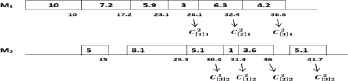
The graph of the completion times of three jobs on two machines and levels

For results on the problem without the learning effect, the reader may refer to ^36–40.

3. The performances of four algorithms

The proposed problem is NP-hard since the classical total completion time minimization problem on m-machine flowshop without learning effect or reentrant consideration is NP-complete ⁴¹. It becomes not economic to facilitate a searching procedure for the optimal solution when the number of jobs is getting larger. Therefore, it has a good advantage policy to consider an effective heuristic or meta-heuristic for a good quality solution. Meanwhile, the literature indicates that a lot of researchers have paid more attention on constructing accurate algorithms within a limited amount of time for solving the classical total completion time minimization problem on m-machine flowshop problem such as Rajendran and Ziegler ⁴², Woo and Yim ⁴³, and Framinan and Leisten ⁴⁴. Nawaz et al. ⁴⁵ proposed a NEH heuristic for the makespan problem. Later, they modified the procedure for the flow time criterion. For simplification, it is referred to the four heuristics as RZ, WY, FL, and NEH, respectively. The main goals of this study is that in the first stage we first adopt four existed heuristics (the RZ, WY, FL, and NEH) for this problem; in the second stage we then use the same four methods combined with three local searches to solve the proposed problem; and in the last stage we develop a heuristic-based genetic algorithm seeded with four good different initials obtained from the second stage to find near-optimal solutions. Specifically, we are interested in investigating the impacts of learning effect and re-entrant times to the performances of all the proposed heuristics considered when the relative parameters are changed.

In what follows, we first evaluate the performance of the four heuristics proposed by Framinan and Leisten ⁴⁴, Nawaz et al. ⁴⁵, Woo and Yim ⁴³, and Rajendran and Ziegler ⁴² in solving the re-entrant permutation flowshop scheduling problem with a position-based learning effect to minimize the total completion time. The algorithms are coded in FORTRAN and run on a personal computer with an Intel(R) Core(TM)2 Quad CPU 2.66GHz with 4GB RAM.

In the tests the job processing times for each level are randomly generated from a uniform distribution [1, 100]. The number of jobs n is set to 8 and 10, the number of machines m at 2, 3, 5, and 10, and the number of re-entrant times l to 2, 3, and 5. The learning index a is also set to 70%, 80%, and 90%, which correspond to a = – 0.515, – 0.322, and – 0.152, respectively, according to Biskup’s ⁴ model. In the tests, we first modify Pji=∑k=1lpjik as the processing time of job J_j on machine M_i, and then apply the FL, NEH, WY, and RZ rule to yield the sequence. As a result, we tested a total of 72 cases with 100 instances in each case.

For the small number of jobs, we use full enumeration method to solve the instance to find an optimal solution. We then compared the solutions obtained by all the heuristics or the GA algorithm in terms of the percentage error, given by

where V_i is the objective value obtained by algorithm H_i and V^* is the optimal objective value obtained by full enumeration. For each case, we recorded the mean percentage error. Tables 1–2 summarize the results.

Fig. 1.

The performance of four algorithms when l changes (n=8 and 10)

As shown in Tables 1–2 and Figure 2, on an average, the mean percentage errors of the FL, NEH, WY, and RZ become large as the number of machines increases. On average, the mean error percentages of the FL, NEH, WY, and RZ are 6.273 and 6.791, 6.135 and 6.730, 6.370 and 7.026, and 6.262 and 6.758 at n=8 and 10, respectively. The results show that NEH keeps slightly better than FL, WY, and RZ.

Fig. 2.

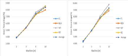
The performance of four algorithms when m changes (n=8 and 10)

As shown in Tables 1–2 and Figure 3, on an average, the mean percentage errors of the FL, NEH, WY, and RZ decline as the learning effect becomes weak. On average, the mean error percentages of the FL, NEH, WY, and RZ are 6.273 and 6.791, 6.135 and 6.730, 6.371 and 7.026, and 6.262 and 6.759 at n=8 and 10, respectively. The results show that NEH still performs slightly better than FL, WY, and RZ.

Fig. 3.

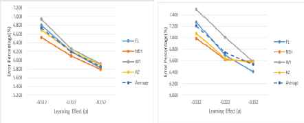
The performance of four algorithms when a changes (n=8 and 10)

On average, NEH with mean error percentages of 6.135 and 6.730 performs slightly better that FL with 6.273 and 6.791, WY with 6.370 and 7.026, and RZ with 6.262 and 6.758 at n=8 and 10 from Tables 1 and 2.

However, as mentioned in Demsar ⁴⁶, Garcia and Herrera ⁴⁷, the non-parametric tests should be preferred over the parametric ones in machine learning field. Therefore, some non-parametric statistical methods, such as the Friedman test, Iman and Davenport test, and post-hoc multiple comparison methods, such as, Nemenyi test, Holm procedure, and Shaffer static procedures ⁴⁷, are employed in analyzing the experimental data for this study. For more works involving with the experimental analysis in the field of evolutionary algorithms, we refer readers to ^48–53.

The numbers (1, 2, 3, 4) in parenthesis in the Tables 1 and 2 show the overall process of computation of average rankings of AEPs for the four algorithms. Friedman test, and Iman and Davenport tests ⁴⁷ check whether the observed average ranks differ significantly from the mean rank R_j=2.5, j=1, 2, 3, 4. Friedman test statistic, in this case, is 23.6787 (with chi-square distribution and degrees of freedom 3), while the critical value χ0.05;32=7.815. Iman and Davenport test statistic, in this case, is 2.7566 (with F distribution and degrees of freedom (3, 71·3=213)), while the critical value F_0.05,3,213 = 2.647.

Owing to both test statistics are greater than the respective critical values at the level of significance α=0.05, a post-hoc tests can be proceeded to detect significant pairwise differences among the search quality obtained from the four algorithms, FL, NEH, WY, and RZ. For this purpose, we have to compute the corresponding statistics and p-values. The test statistics, as Demsar ⁴⁶, for comparing the i-th and j-th algorithm is z=(Ri−Rj)/k(k+1)/(6N) where R_j is the observed average rank computed through the Friedman test for the i-th algorithm, k=4 is the number of algorithms to be compared, and N=72 (that is N= n·l·m·a = 2·3·4·3) is the number of parameter combinations (each parameter combination is treated as a “block”) used in the comparison. The four observed R_j’s, computed in Table 2, for the FL, NEH, WY, and RZ are 2.243, 2.236, 3.132, and 2.389, respectively. Note that the standard error in the pairwise comparison between two algorithms is SE=k(k+1)/(6N) = [(4 · 5)/6 · 72]^1/2 = 0.2152.

Table 3 presents the family of hypotheses ordered by their p-values and the adjustments of α by Nemenyi’s (α_NM), Holm’s (α_HM) and Shaffer’s static (α_SH) procedures. In order to take multiple tests into account and to be compared directly with any chosen significance level α, the corresponding adjusted p-value (APV) procedures, Nemenyi (APV_NM), Holm (APV_HM), and Shaffer’s static (APV_SH) are also employed in this study. The computing formulas refer to Garcia and Herrera (2008). These values are included in the last three columns of Table 3.

As shown in Table 3, it is obvious that Nemenyi’s test, Holm’s procedure and Shaffer’s static procedure reject the hypotheses [i=1 to i=3] consistently. Since these three hypotheses all include the algorithm WY and the average rank of WY (3.312) is the largest among the four average ranks, it can be concluded that the algorithm WY performs worse than any of the other three algorithms does. Besides, the performance of three algorithms, NEK, FL and RZ, is not significant at the level of significance α =0.05. Moreover, the three APV’s conform the same conclusion at α=0.05.

4. The four algorithms combined with three local searches

It can be observed in Section 3 that on average the mean error percentage of all the four algorithms is more than 6% because of the re-entrant factor being brought up. In order to get a good quality solution, we build 12 heuristics by combining FL, NEH, WY, and RZ with three local search methods that are effective in treating the flowshop scheduling problem, namely the pairwise interchange, backward-shifted re-insertion, and forward-shifted re-insertion ⁵⁴. For example, the proposed heuristics in FL algorithm improved by the pairwise interchange, backward-shifted re-insertion, and forward-shifted re-insertion are recorded as FL_PI, FL_EBSR, and FL_EFSR, respectively. The others are similar to the front. The tested results of all the proposed heuristics are reported in Tables 4–5.

It can be seen in Tables 4 and 5 that the heuristics with the pairwise interchange method outperform than those with backward-shifted re-insertion or forward-shifted re-insertion in terms of the numbers of cases, i.e., 124 cases for PI while 3 and 17 cases for backward-shifted re-insertion and forward-shifted re-insertion at n=8, while 136 cases for PI while 2 and 6 cases for backward-shifted re-insertion and forward-shifted reinsertion at n=10. On an average, among four heuristics, FL algorithm improved by PI method is slightly better than those with backward-shifted re-insertion and forward-shifted re-insertion in terms of mean error percentage. So do the NEH, WY, and RZ algorithms in Tables 4 and 5. On average, the results indicated that FL improved by PI method with the mean error percentages of 2.436 at n=8 and 2.993 at n=10 are smaller than each of other three algorithms improved by PI method.

5. Four heuristic-based genetic algorithms

As stated in the previous section, FL improved by PI method with the average mean error of less than 3% outperforms the other three algorithms with PI method. However, it can still be seen in Table 4 that some case has a bit bigger mean error percentage of 4.649. In view of this situation, we attempt to use a heuristic-based genetic algorithm further to improve near-optimal solutions. Literature releases that the genetic algorithm (GA) has been widely and successfully used in many combinational problems ^55–61. It can be seen that the initial populations are generated randomly in GA settings ⁶². However, some research suggests that it is a good idea to construct the initial population based on other heuristics that makes GA to yield the good quality solution more quickly ^63–66. In light of this observation, this study will adopt four heuristics as initial sequences in GA algorithm which are included FL_PI, NEH_PI, WY_PI, and RZ_PI. The main steps of the proposed GA are summarized in the following.

Genetic algorithm process:
• Step 1:

  Representation of structure- a sequence of the jobs presents a structure in the problem that is followed by Etiler et al. ⁶⁵.

• Step 2:

  Initial population- We apply four heuristics as initial sequences in GA. In first one, FL algorithm is improved by PI method which is recorded as FL_PI+GA. The second, third, and fourth genetic algorithms, denoted as NEH_PI+GA, WY_PI+GA, and RZ_PI+GA, are the NEH, WY, and RZ algorithms improved by PI method, respectively.

• Step 3:

  Population size- We adopt an initial population and create other members by using an interchange mutation operator up to population size ⁶⁴. In a preliminary trial, the population size N is set at 20 in our computational experiment.

• Step 4:

  Fitness function- The fitness function of the strings can be calculated as

  g(Si(v))=max1≤k≤N{∑j=1nCjmR(Sk(v))}−∑j=1nCjmR(Si(v)),

  where S_i (v) is the ith string chromosome in the v-th generation, ∑j=1nCjmR(Si(v)) is the total completion time of S_i (v), and g(S_i (v)) is the fitness function of S_i (v). The probability, P(S_i (v)), of selection for a schedule can be calculated as P(Si(v))=g(Si(v))/∑k=1Ng(Sk(v)). This is also the criterion used for the selection of parents for the reproduction of children.

• Step 5:

  Crossover- Following by Falkenauer and Bouffouix ⁶⁷, Etiler and Toklu ⁶⁸, Etiler et al. ⁶⁵, we adopt linear order crossover (LOX) method in each GA. In order to protect the best schedule which has the minimum total completion time at each generation, we transfer this schedule to the next population with no change, or the crossover rate P_c = 1.

• Step 6:

  Mutation- The mutation rates (P_m) are set at 0.25 based on our preliminary experiment.

• Step 7:

  Selection- In each GA, the population sizes are set to 20 from generation to generation. Excluding the best schedule which has the minimum total completion time, the other offsprings are generated randomly from the parent chromosomes by the roulette wheel method.

• Step 8:

  Stop rule- Each GA is terminated after 1000 generations in our preliminary experiment.

We conducted computational experiments to test the performance of the four meta_heuristics FL_PI+GA, NEH_PI+GA, WY_PI+GA, and RZ_PI+GA in solving the re-entrant permutation flowshop scheduling problem by using the same data. All results are reported in Tables 6 and 7.

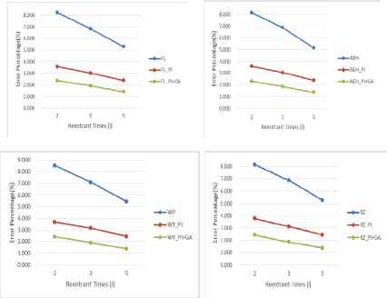
As shown in Tables 6–7 and Fig. 4, on an average, the mean percentage errors of FL_PI+GA, NEH_PI+GA, WY_PI+GA, and RZ_PI+GA decline as the reentrant number becomes larger. On average, the mean error percentages of FL_PI+GA, NEH_PI+GA, WY_PI+GA, and RZ_PI+GA are only 1.048 and 1.904, 1.109 and 1.845, 1.112 and 1.893, and 1.040 and 1.893 at n=8 and 10, respectively. The results show that FL_PI+GA and RZ_PI+GA are only slightly better than NEH_PI+GA and WY_PI+GA. So do the similar trend for the performances when changing the numbers of machines or the learning effect. In addition, it can be observed in Tables 6–7 and Fig. 4 that the mean error percentage can be declined sharply by these improvements for four algorithms no matter what the reentrant time or number of machine or learning effect changes.

Fig. 4.

The performance of four and their improved algorithms when l changes (n=10)

6. Four heuristic-based genetic algorithms on the larger number of job

In the tests we randomly generated the job processing time for each level from a uniform distribution [1, 100]. We set the number of machines m at 2, 3, 5, and 10, and the number of re-entrant times l at 2, 3, and 5. We also set the learning index a at 70%, 80%, and 90%. As a result, we tested a total of 72 cases with 100 instances in each case.

For the cases with a large number of jobs, i.e., n = 50 and 100, we first solved each instance by using the eight heuristics FL_PI, FL_PI+GA, NEH_PI, NEH_PI+GA, WY_PI, WY_PI+GA, RZ_PI, and RZ_PI+GA algorithms to obtain near-optimal solutions. We measure the performance of a heuristic or an GA algorithm in terms of the relative percentage deviation (RPD), defined as

where V is the objective value obtained by a heuristic or a GA and V_min is the best solution among FL_PI, FL_PI+GA, NEH_PI, NEH_PI+GA, WY_PI, WY_PI+GA, RZ_PI, and RZ_PI+GA algorithms. For each case, we recorded the average (denoted as RPD) percentage deviation. Tables 8–9 summarize the results. We see from Tables 8 and 9 that the RPDs of FL_PI+GA, NEH_PI+GA, WY_PI+GA, and RZ_PI+GA have a decreasing trend when the re-entrant time increases as shown in Fig. 5, but have an increasing trend when the number of machines becomes big or the learning effect gets stronger as shown in Fig. 6 and 7. The results indicate that FL_PI+GA performs better than the other three heuristics regardless of the number of re-entrant times or machines or learning effect. In addition, there is no clearly dominance relationship between NEH_PI+GA and WY_PI+GA from Figs 5–7.

Fig 5.

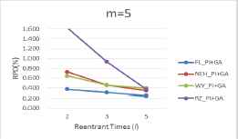
The performance of four GA algorithms when l changes (n=100, m=5)

Fig. 6.

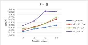
The performance of four GA algorithms when m changes (n=100, l=3)

Fig. 7.

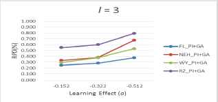
The performance of four GA algorithms when a changes (n=100, l=3)

Furthermore, from Tables 8–9, it can be observed that on average FL_PI+GA has smaller RPD values of 0.465% at n = 50 and 0.327% at n = 100, which are better than those of NEH_PI+GA of 0.646% and 0.530%, of WY_PI+GA of 0.666% and 0.633%, and of RZ_PI+GA of 0.829% and 0.769% at n = 50 and 100, respectively. And, Fig. 8 releases that the RPD of FL_PI+GA has the least dispersion among the four GA algorithms.

Fig 8.

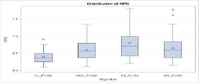
The RPD distributions of four GAs (n=50, 100)

As shown in Fig. 9, Box plots convey the information contained in Tables 6 and 7. It is obviously shown the difference between search results for the twelve algorithms constructed in the three stages. The applied heuristics, especially the GAs used in the third stage, improve considerably the quality of the search solutions. Overall, it is concluded based on the above discussions that the FL_PI+GA algorithm does well and it might be adopted to solve the proposed problem in view of its stability and its ability in producing near-optimal solutions.

Fig 9.

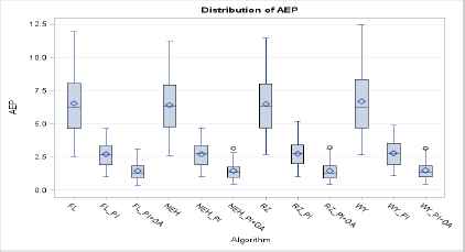
AEP distributions of twelve algorithms (n=8, 10)

However, as done in Section 3, we employ non-parametric statistical tests to check whether there exists any significant difference among the performances of the four GA-based algorithms for the large size of jobs. The numbers (1, 2, 3, 4) in parenthesis in Tables 8 and 9 show the overall process of computation of average rankings of RPDs for the four GA-based algorithms. The four observed R_j’s, computed in Table 9, for the FL_PI+GA (FGA), NEH_PI+GA (NGA), WY_PI+GA (WGA), and RZ_PI+GA (RGA) are 1.153, 2.500, 3.403, and 2.944, respectively. The notations and formulas are omitted since they are the same as those used in the Section 3.

Friedman test, and Iman and Davenport tests check whether the observed average ranks differ significantly from the mean rank R_j=2.5, j=1, 2, 3, 4. Friedman test statistic, in this case, is 122.15 and the correspondent critical value, at α=0.05, is χ0.05;32=7.815. Iman and Davenport test statistic, in this case, is 95.46 and the correspondent critical value is F_0.05,3,213 = 2.647. Given these test statistics are greater than the respective critical values, there are significant differences among the observed results from the four GA-based algorithms. Thus, a post-hoc statistical analysis could help to detect specific differences among the search quality obtained from the four GA-based algorithms.

As shown in Table 10, it can be seen that Nemenyi’s test rejects the hypotheses [i=1 to i=4], Holm’s procedure and the Shaffer’s static reject the hypotheses [i=1 to i=4, and i=6]. Besides, All three APVs reject the hypotheses [i=1 to i=4] at level of significance 0.05. Therefore, it can be concluded that the algorithm FL_PI+GA (FGA) performs significantly better than any of other three GA-based algorithms does, and NEH_PI+GA (NGA) performs significantly better than WY_PI+GA (WGA) does.

7. Conclusions

In this study we address the re-entrant permutation flowshop scheduling problem with learning considerations to minimize the total completion time. Given the intractability of the problem, we build four heuristics based on three local search methods to approximately solve the problem. Moreover, in order to find good quality near-optimal solutions, we apply genetic algorithm using the solutions obtained by the heuristics as initial solutions to solve the problem. The computational results show that the GA algorithm seeded with the solution obtained by combining FL algorithm improved by interchange method performs best in terms of solution quality. Future research may consider including the due dates to solve the problem involving other scheduling objectives such as the total tardiness.

Acknowledgements

The authors are grateful to the Editor and anonymous referees for their many helpful comments on the earlier versions of our paper. This paper was supported by the NSC of Taiwan under grant numbers MOST 105-2221-E-035-053-MY3 and MOST 103-2410-H-035-022-MY2.