
Location, Allocation and Routing of Temporary Health Centers in Rural Areas in Crisis, Solved by Improved Harmony Search Algorithm
- DOI
- 10.2991/ijcis.2017.10.1.60How to use a DOI?
- Keywords
- disaster relief logistic; harmony search algorithm; temporary health centers; vehicle routing problem; rural areas
- Abstract
In this paper, an uncertain integrated model for simultaneously locating temporary health centers in the affected areas, allocating affected areas to these centers, and routing to transport their required good is considered. Health centers can be settled in one of the affected areas or in a place out of them; therefore, the proposed model offers the best relief operation policy when it is possible to supply the goods of affected areas (which are customers of goods) directly or under coverage. Due to that the problem is NP-Hard, to solve the problem in large-scale, a meta-heuristic algorithm based on harmony search algorithm is presented and its performance has been compared with basic harmony search algorithm and neighborhood search algorithm in small and large scale test problems. The results show that the proposed harmony search algorithm has a suitable efficiency.
- Copyright
- © 2017, the Authors. Published by Atlantis Press.
- Open Access
- This is an open access article under the CC BY-NC license (http://creativecommons.org/licences/by-nc/4.0/).
1. Introduction
In many situations and especially when rural areas are affected in disaster, many villages lose their communication and transportation paths, but since the locations are very close to each other it is possible for a temporary health center to provide services for several places near each other. On the other hand, during the early hours of crisis, it is very difficult to estimate the damage and it is actually impossible to determine the exact rate of demands. Therefore, it is quite logical to consider the assumption of uncertainty on the values of parameters.
Finally, a key parameter that plays a significant role in relief efforts during the crisis is time. Saving the time in relief efforts can have a significant effect on reduction of casualties.
In this paper, an integrated model of locating temporary health centers in the affected area, allocating the affected areas to these centers and routing the required goods in such centers is presented. Since the time of vehicles’ arrival to the relief centers is much more important than their return time to the central depot, the open routing is used in the model. Objective function of presented model is to minimize the time to reach the last visited relief center. Moreover, as the determining of exact demand for basic commodities during disasters is very difficult and in many cases it is impossible, uncertainty of demand has been considered in the suggested model and in order to deal with uncertainty, the fuzzy credibility theory has been applied. Finally, with regard to NP-Hard nature of the problem, a metaheuristic algorithm based on harmony search algorithm is proposed to solve the problem in large scales and its performance has been compared with basic harmony search algorithm and variable neighborhood search algorithm.
In continue, in the section 2 of the article, the literature is reviewed. In section 3, the fuzzy theory is introduced. In section 4, the fuzzy credibility theory is introduced. The mathematical model of the problem is discussed in section 5. Section 6 is related to the suggested solution methods. Numerical results are presented in section 7 and finally conclusion is presented in section 8.
2. Literature Review
Research on the transport of relief items for the first time traces back to the one conducted by Knott in 1987 [1]. Having limited resources, Knott modeled the conditions in which a number of different vehicles are in a warehouse and the objective is to minimize the lost demands.
Obviously, at the onset of crisis,transport infrastructures are unreliable for relief supplies;that is why Barbarosoğlu et al. (2002) [2] modeled the flight and rescue operations plan of helicopters. The issue is divided into two levels: the first level deals with tactical decisions including the management of fleet and pilots and determining the number of tours covered by each helicopter. The second level deals with making operational decisions including the routes planning, loading and unloading, rescue and refueling of the helicopters.
Özdamar et al. (2004) [3] investigated logistic planning in emergencies for shipping goods to distribution centers in affected areas. The developed network in this research has investigated a dynamic time-dependent transport issue and has repeatedly provided responses at the given time intervals for delivering aids.
Sakakibara (2004) [4] studied the flow of goods in road networks during the response to crisis where the roads have been divided into separate components. The author has used topological indices to quantify the capability of accessing roads network. Then, he has divided the crisis areas into separate pars and has introduced a methodology to determine the effective means of communication and transportation in order not to separate operations in the regions.
In order to assist the government agencies, Chang et al. (2007) [5] have proposed two randomized planning models to determine the storage of rescue resources and the required rescue equipment in them and distribution of rescue equipment. The first model aims to minimize the distance from the rescue equipment and the second model aims to minimize deployment costs and the average cost of rescue equipment.
Rawls and Turquist (2010) [6] offered a two-step contingency planning model that combined facility locating and making decision on the storage level of relief items with uncertainty of demands, pre-stored items and the position of transportation network in any event.
Mete and Zabinsky (2010) [7] offered a two-step contingency planning model that specified the location of warehouses and inventory levels. The objective function of their model minimizes transportation duration and unsatisfied demands.
Özdamar et al. (2011) [8] presented a mathematical model for logistic planning of helicopters for transportation of injured victims and treatment goods. In the cited model, the vehicles were merely helicopters to minimize the total time of the mission of such vehicles to supply the required goods for victims. This model has also tried to consider the loading time an addition to the travel time.
Walter and Gutjahr (2014) [10] have offered a routing and locating model for relief operations during the disasters. They have stated that middle warehouses should be built temporarily, so that the relief operations and supplying the needs of injured people can be done more quickly. They offered a three-objective model to minimize short term and medium costs and to maximize the shipment of humanitarian goods. They have solved the model using epsilon restriction model and have compared the results with the meta-heuristic solution method of variable neighborhood search (VNS).
The use of covering tour is the approach that has been applied by some researchers in the field of relief operations during the crisis. The important point here is that in most of the research, the coverage radius is considered to be very small so that the individuals’ needs can be met in the shortest time and distance from them.
Doerner et al. (2007)[11] tried to minimize the unmet demands in critical situations using the covering tour. In their proposed model, a central depot was used and then locating medical centers and routing a vehicle for supplying their needed goods were emphasized. Moreover, the small villages with low population and short distances from each other were considered as demand places.
Nolz et al. (2010)[12] offered a two-objective model to deliver food and medicine and to provide shelter for the affected areas. The proposed model tries to determine the goods distribution method in the affected areas based on the coverage issue. In order to solve the model, a genetic algorithm has been developed based on the neighborhood search.
Azimi et al. (2012)[13] proposed a model for locating central relief spots and routing their supplies. They stated that in many cases rescue equipment could not visit all places. Therefore, relief operation centers are located in a short distance from them so that the needy people refer to those centers and receive their required products. All the demands must be met and all the relief spots should be located in such a way that all the demand points are placed in distances shorter than the maximum permitted distance from a relief center. In the presented model, the goods of the centers are supplied via a central depot and by similar transportation means. The purpose of vehicles routing model is to minimize the total distance traveled by the vehicles.
Abounacer et al. (2014)[14] continued the research conducted by Yi et al.[15]. In relation to the location, researchers have considered determining the number of relief centers and humanitarian distribution, their positions, and functions. In relation to routing, the vehicles are responsible to transport goods from the distribution centers to the demand points. Three various objectives are considered for this issue: first, to minimize the total time of goods transport; second, to minimize the number of required centers; third, to minimize unmet demands.
Tofighi et al. (2015) designed a humanitarian logistics network for crisis situations by taking into account the factor of uncertainty. This article was focused on locating the multi-purpose warehouses and relief supply distribution centers while optimizing the routes of relief vehicles. In this model, uncertainty in demand and availability of routes were formulized by fuzzy logic, and given the presence of two uncertain parameters, the formulation was carried out from the combined uncertainty perspective. Thus, the resulting mathematical model was solved through a two-stage approach. The numerical analysis of this study was based on a hypothetical strong earthquake in Tehran [31].
Kanahi et al. (2016) developed a two-stage model for location and routing during a crisis under uncertain conditions. In this model, the aim was to reduce the risk of disaster relief, which was defined in terms of unmet demand. This model was converted to a single-stage equivalent model and was solved by a heuristic method [32].
Phantom et al., (2016) formulated the problem of designing a relief network and solved it by a decomposition-based heuristic. They examined the problem of locating emergency stocks and routing basic supplies in a crisis situation. The problem formulated for such situation, where demand is partly uncertain, was solved by the use of a heuristic method based on decomposition of variables [33].
By survey past researches in the field of disaster relief, the distinction of this article with other research on the simultaneous optimization of location, routing and assignment in terms of demand uncertainty and crisis by using novel metaheuristic methods. Also consider the covering radius of the relief centers in order to service the affected areas to the nearest relief centers, is another new aspect of the research and innovation of it than other research. On the other hand with respect to the importance of time in relief towards the cost, the aim of this research is to optimize latest relief time. This is less the case in research of interest to other researchers.
3. Fuzzy theory
A classic collection is normally defined as a set of its members. Each data by itself can be a member of this collection or not. Consequently, membership or lack of membership of any data is clearly identified, but in some collections, membership is not associated with certainty. Fuzzy theory is used in dealing with such collections. Fuzzy set theory was first introduced by Zadeh[16] and was developed for different issues. Moreover, fuzzy variable was first introduced by Kaufmann [17]and then by Zadeh [18]and Nahmias[19]. Liu[20] realized the credibility function in his studies. In this section, the basic concepts of fuzzy set and fuzzy measurement are discussed.
If we consider the fuzzy number
If
Here, the credibility of a fuzzy event is defined as the mean of its possibility and requirement. A fuzzy event might fail even if its occurrence possibility is equal to one and it might occur even if its requirement is equal to zero. That is why the credibility criterion uses the combination of these two functions and in fact plays the role of occurrence possibility in fuzzy conditions[21].
Accordingly, the demand of a customer is not less than d1 and not more than d3 and d2 is the most reasonable value for the customer demand. According to the above definitions, the functions of possibility, requirement, and credibility are rewritten as the following.
4. Application of credibility function
In order to estimate the customer demand, the credibility method is used in this article. To do so, a credibility level is considered and the rate of customers’ demands is estimated accordingly and then the routing is done based on the estimated demand. Finding the optimum amount of Cr will have a decisive role in the real amount of objective function of the problem. Determining the primary amount of customers’ demands based on credibility is an estimation and when the vehicles are trying to supply the demands of relief operation centers, they certainly can face demands that are different from the predetermined ones. Selecting small amounts of credibility causes the amounts considered for the customers’ demands to be estimated with minimum possible amounts. This reduces the response time but there is the possibility of failure in routes because the estimated rate of demand might be greater than its real rate. Failure means that in order to supply the demands of other customers of its tour, the vehicle has to return to the depot and do replenishment. On the other hand, selecting large amount of credibility causes the upper level of demand to be selected for the customer. This makes the routes found for the problem remain stable in this case and prevents the possibility of not responding the customer’s needs. In this situation, due to overestimation of customers’ demands, the capacity of vehicles has not been used properly and the response time might increase. To find the best amount of credibility according to which the rate of customers’ demands can be estimated, it is necessary to make use of Stochastic simulation [21].
4.1. Determining Optimal Credibility level
In order to obtain the optimal amount of Cr parameter the following algorithm which is presented in references [21,22] is utilized.
Step one: for Cr=0:0.1:1 repeat steps two to five.
Step two: specify the customers’ demands in the selected Cr level and find the optimal solution to the problem.
Step three: run the sub program for generating random numbers to clarify the demands of affected areas.
Sub Program of Generating Random Number
Sub step one: i=1
Sub step two: generate a random number of m between the high and low limit of the fuzzy number of the demand of i point and specify the amount of its membership degree (f) based on the membership function of the demand of the affected area i.
Sub step three: produce the random number of r in [0, 1] interval.
Sub step four: if r ≤ f, introduce mi as the real amount of the demand of I point and go to step 4; otherwise, go to step 2.
Sub step five: increase i one unit. If i ≤ n go to sub step 2; otherwise, go to sub step 6.
Sub step six: end.
Step four: with regard to the simulated demand of affected areas calculate the cost of optimized tours at specified Cr level. Consider the cost of occurred failures in calculating the length of tours.
Step five: do steps three and four 1000 times and calculate the mean of costs.
Step six: Report Cr content with lowest mean of objective function as the optimized Cr.
5. Problem definition
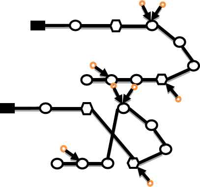
In this paper, an integrated model of locating temporary health center s in the affected areas, allocating affected areas to these centers, and routing their required good is offered. Since in disasters supply the immediate needs of the victims and providing their medical goods and treatments are particularly important, the paths are considered open and the purpose of proposed model is to minimize the time of providing services to the last affected area. Relief centers can be settled in one of the affected areas or in a place out of them; therefore, the proposed model offers the best relief operation policy when it is possible to supply the needs of affected areas directly or under coverage. In other words, the demands of different places can be delivered in the same place they are located or in they can be carried to another place located at a reasonable distance from them so that individuals can receive their relief goods by traveling a short distance. This approach is very applicable for crises involving the rural areas. In this issue, the impossibility of establishing relief operation centers in some affected areas due to the possibility of occurrence of some future events such as aftershocks, fire, etc. is considered. The duty of relief centers is to meet the demands of affected people in such areas for essential goods and medicine. Fig.1. is presented for better expression of the problem.
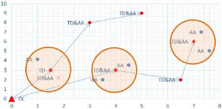
An example of 11 affected areas
Abbreviations DC, TD, AA, and BA in Fig. 1. respectively stand for distribution center, temporary health center s, affected area, and barrier area for the establishment of temporary centers. In this example, 6 temporary health center s have been established to aid the affected areas. Five centers out of the six are located in the affected areas and one center is settled in the central point. Since in critical situations the establishment of such centers in the shortest possible time is considered, the centers are assumed to be settled as outpatient centers and the cost of establishing them is discarded. On the other hand, the required goods of such relief centers are supplied by a central depot. The good is carried to the places where the relief centers are located by vehicles with specified capacity and the demands of visited areas and the areas supported by them are met. In many disasters, it is very difficult to determine the exact amount of required goods (demand) and application of probabilistic models with regard to lack of sufficient data is actually impossible. Therefore, in this paper, the demand of each affected area is considered as a fuzzy number with a triangular membership function.
5.1. Mathematical modeling
In this section, an integer linear programming model is introduced to formulate the defined problem.
The following assumptions have been considered in this model:
- •
It is a single-commodity model.
- •
Each relief center receives goods only from one vehicle.
- •
Central depot covers no point. In fact, the depot is too far from the affected areas.
- •
The affected areas receive their needed goods only from one relief center.
- •
The whole demands of all affected areas must be met.
- •
The time to travel a distance is the same for all the vehicles and all of them have equal capacity.
- •
There are some middle points that are not demand points but their distance from the demand points is very little and it is possible to establish temporary depot there.
- •
It is not possible to establish temporary depot in some affected areas.
The sets considered in this model are as the following:
is the set of all points R′ = {1,2,…R,R + 1}, the point of one is depot and the point of R+1 is virtual. is sub set of R ′ which consists of affected areas (customers of first aid product) is the set of affected areas (points with demand) where it is impossible to establish relief centers (barrier areas). Is the set of vehicles K′ = {1,2,…, K}.
The model parameters are presented below.
The time to travel between two points i and j Fuzzy demand of point i Maximum coverage distance Binary parameter which is equal to 1 if the distance between point i and point j is less than dismax Vehicle capacity a large number
The variables in the model are as the following:
is equal to 1 if the distance between two nodes i and j is traveled by vehicle k; otherwise, it is equal to 0 is the collected demands at point i i ∈ {2,3,.., R} is equal to 1 if point i is visited by one of the vehicles; otherwise, it is equal to 0 i ∈ {1,2,.., R} is equal to 1 if the demand of point i is met by the visited point j; otherwise, it is equal to 0 The time when vehicle k reaches point i the time when the good is delivered to the last relief center, in continue, the mathematical model is described as follow:
Eq. (8) is the objective function of the model which is considered to minimize the time to reach to the last relief center. Constraint (9) states that vehicles only pass through the points where the temporary depots are established. Constraints (10) and (11) indicate that all the vehicles should leave the depot and they cannot return there. Constraints (12) and (13) state that all the vehicles should enter the virtual node (R+1) and no vehicle should leave the node. Constraint (14) states that if a vehicle enters a node, it should leave there. Constraints (15) and (16) state that every affected point should be allocated to a temporary center. Constrains (17) and (18) are related to the capacity of vehicles. Constraint (19) refers to the point that if there are some demands in the visited point, they should not be met by another point within its coverage distance. Constraint (20) guarantees that temporary health center s are not established in inappropriate places. Constraints (21) and (22) are related to omitting the sub tour and calculating the time to reach the temporary health center s. Constraints (23) and (24) identify the type of decision variables.
5.2. Virtual node
In order to model open tours, a virtual node R+1 has been used initiatively. The distance between this node and other points is 0 and all the vehicles after passing the determined point do not return to the origin but go to this virtual node. It is possible to calculate the time to reach the last traveling point using the virtual node. It should be mentioned that the time of receiving to the last point in each tour is equal to the time to reach the virtual node of R+1.
6. Solution methods
In this section, the proposed solution methods are presented. First, the basic harmony search is explained. Then, the improved search algorithm is offered and ultimately, the variable search algorithm is explained.
6.1. Harmony Search Algorithm
Due to its applicability for continuous and discrete optimization problems, low mathematical calculations, simple concepts, few parameters and easy implementation, harmony search (HS) algorithm has become one of the appropriate applicable optimization algorithms in various problems in recent years [23]. Compared to the other meta-heuristic methods, this algorithm has fewer mathematical requirements and can be matched with changes in parameters and performances in different engineering problems[24]. In summary, the steps of HS can be stated as the following:
Step one: Setting the parameters of the problem and algorithm
In this algorithm, like the other meta-heuristic algorithms, it is necessary to initialize problem and algorithm parameters. HS parameters include harmony memory size (HMS), harmony memory consideration rate (HMCR), pitch adjustment rate (PAR), band width (BW) and number of improvisations (NI).
Step two: Creating random initial values for harmony memory
Each harmony vector is randomly initialized and placed in harmony memory. Then, the objective function for each vector is calculated and stored in HM matrix.
Step three: Creating a new harmony
In order to produce each component of New Harmony, two different approaches are used in this algorithm. In the first approach which is selected with the same probability as the harmony memory consideration rate (HMCR) a component is randomly extracted from among the corresponding components of one of the harmony memory members. After selecting a component with equal probability to the pitch adjustment rate (PAR), the selected component changes randomly. The range of changes is the same as the band width (BW). In the second approach, the component is randomly initialized with the same probability to (1-HMCR).
Step four: Updating harmony memory
If the quality of generated solution is better than the worst solution available in the harmony memory the new solution will replace the worst harmony memory solution; otherwise, the new undesirable solution is eliminated.
Step five: checking stop criterion
The third and fourth steps of algorithm continue up to specified number of improvisation and the best answer is reported as the result to the algorithm [23].
for (j=1 to n) do
r1=a random number of continuous uniform of [0 1]
if (r1< HMCR) then
  Xnew(j) = Xa(j) where a ∈(1,2,…,HMS)
  r2=a random number of continuous uniform of [0 1]
  if (r2< PAR) then
    Xnew(j) = Xnew(j) + r 3 × BW where r3 ∈ (0,1)
  end if
else
    Xnew(j) = LBj + r × (UBj -LBj), where r ∈ (0,1)
  end if
end for
Algorithm 1.Pseudocode of HS‘s creating new harmony
Despite the suitability of HS, in some cases it converges quickly. Moreover, this algorithm with a greedy nature is looking forward to improving the worst responses available in harmony memory which in turn causes the diversity of responses in harmony memory to decrease and be trapped by local optimum [24].
Considering the mentioned difficulties for the HS, the required changes for the development of this algorithm and its efficiency are discussed. In part 6.2 changes applied to HS are explained.
6.2. Improvement of basic HS
In order to improve the quality of HS, four main changes are implied in it as follow.
- I)
In new solution generation step in basic algorithm, each component of the new harmony vector is randomly selected from their corresponding components in the harmony memory. However, in new method first a harmony is selected randomly from among harmony memory. For each component of the selected harmony with HMCR probability, it is replaced by the components of one of the members of harmony memory. To do so, with the same probability as HMCR, the rate of component is selected by fitness distance ratio (FDR) which was first introduced by Veeramachaneni et al[25], and then it is determined randomly by
In this equation, f(xi) and xil are respectively the objective function and the new answer component; f(xj) and xjl are the objective function and the selected member of harmony memory.
- II)
Pitch adjustment ratio is not randomized and is done in such a way that the new answer components move towards the best available response. After selecting a component randomly, with (PAR) probability it move towards the corresponding component within the best answer available in the harmony memory.
In equations (28) to (30), f (best) and f (worst) are respectively the best and the worst answers available in the harmony memory.
In Eq. (32) xbestj and xij are respectively the rates of j component from the best answers available in harmony memory and selected answer. Given the presented trend for the rate of band width (BW) the more appropriate the selected solution is, a shorter step it takes towards the best solution in the harmony memory, but if the selected solution has an inappropriate objective function it takes longer steps towards the best answer available in harmony memory.
- III)
In order to improve the New Harmony, local search is used.
In this step, the innovative local search between two tours which is explained in 6.4.2. is used to improve the applied response and it is applied to the response as long as the response is not improved.
- IV)
In order to place new solution in harmony memory if the quality of new solution is lower than the worst answer in harmony memory, it is eliminated; otherwise, it is added to harmony memory; then S index is calculated via Eq. (33) and the answer with highest rate of S is eliminated.
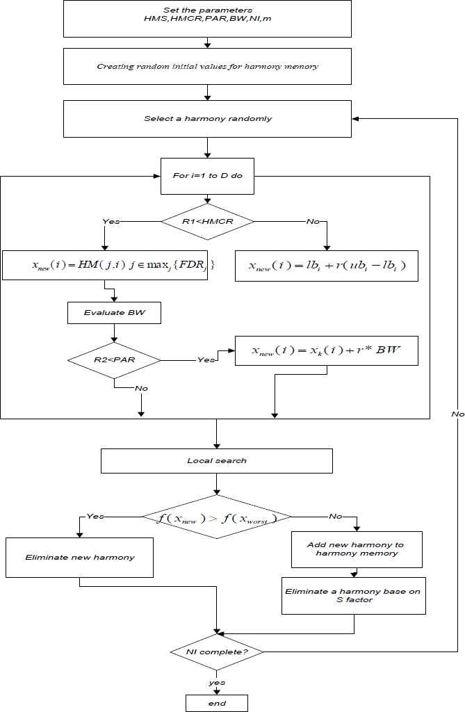
In the S index f (xi−1), f (xi) and f (xi+1) is the cost function of i-1-th, i-th and i+1-th answers in list of answers, sorted non increasingly. The diversity of available solution in the harmony memory increases through this approach. The flowchart of developed HS is displayed in Fig. 2.
flowchart of improved HS algorithm
6.2.1. Solution Representation
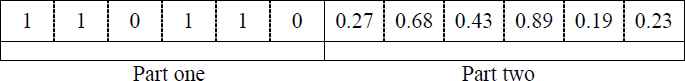
In order to represent each solution (harmony) a two-part string with the length of 2R is used where R is the total number of points. In the first part, 0 and 1 are placed. 1 means the establishment of temporary depot and the movement of a vehicle through that point and 0 means no vehicle passes there. If this point has some demand the failure to pass through it means to cover by a passing point. It should be noted that if one of the inaccessible points is visited the solution is modified. In the second string, numbers are placed in the range [0 , 1] that indicate allocation of the points to vehicles. Therefore, the range of [0 , 1] is divided into K (number of vehicles) equal parts with regard to the range to which the number allocated to i section of the second part belongs to. An example of a solution for a problem with 6 places and 2 vehicles is displayed in Fig. 3. According to Fig. 3. nodes 1, 2, 4 and 5 are selected for establishment of temporary depots. In the second part of the string, the numbers less than 0.5 are allocated to vehicle 1 and the numbers more than 0.5 are allocated to the second vehicle. In other words, the demands of points 1 and 5 are met by the first vehicle and the demands of points 2 and 4 are met by the second vehicle.
an example of the representing the solution
The method of allocating coverage points to passing points is based on the lowest number of coverage so that if a coverage point can supply its demands through several passing points it will chose a point to which the lowest number of coverage points is allocated.
In each solution, determining the vehicles routs between vertical points is done through innovative algorithm based on GENI which is presented in 6.2.2.
Considering such solution representation, it can be claimed that the constraints of the presented model are evaluated. The only constraints that might be exceeded are the constraints of vehicles capacity. In order to increase the search space, the algorithms are not bound to observe the capacity and exceeding the capacity of vehicles is added to the objective function as a penalty.
6.2.2. Rout construction Algorithm based on GENI Algorithm
GENI algorithm or generalized insertion procedure was first introduced by Gander et al. (1992) [26] for travel salesman problem. This algorithm is generated through the combination of two insertion methods and the results indicate that it has good efficiency in the quality and time of solution.
In this algorithm, at first for selected points, three points that create the greatest coverage are selected and the best path between them is selected so initial tour is created. Then, the following insertion procedure is used for the other points.
Suppose that the initial tour is as (v1,v2,…,vi,…,vj,…,vk,…,v1). Also, if node v is the selected node, Np(v) is defined as a set of P nodes in the selected tour that have the shortest distance from v compared with the other nodes inside the tour (P is considered to be equal to (3) and Pij represents nodes between vi and vj in the rout of selected tour.
Sub step 0: Consider node v which is not in the tour.
Sub step 1: select two nodes vi, vj from the set of Np(v) and the node vk from the set of Np(vj+1)\{vi,vj}.
Sub step 3: Remove edges (vi,vi+1),(vj,vj+1),(vk,vk+1).
Sub step 4: add edges (vi,v),(v,vj),(vi+1,vk),(vj+1,vk+1) to the tour.
Sub step 5: Repeat sub steps 1 to 4 for all pairs of the nodes of the set Np(v)and for all the nodes of Np(vj+1)\{vi,vj} and report the best state.
Sub step 6: if there is any node which is not in the tour repeat sub steps 1 to 5.
Finally, two local search methods presented in subsection 6.4 are applied for each solution.
Fig. 4. displays an example of insertion using the above method. Each method continues as long as it improves the solution.
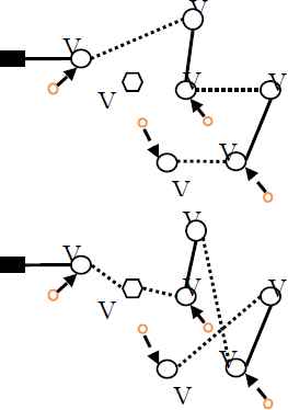
An example of GENI algorithm insertion
6.2.3. Producing initial Solutions
In order to produce initial solutions two innovative procedures have been used. In order to avoid convergence in algorithm and to create diversity in primary solutions, according to the tests 400 solutions are produced through each heuristic algorithm. Moreover, 200 primary solutions are produced randomly. Then, the best produced solutions are selected equal to the number of vectors of harmony memory size (HMS) and are introduced as the primary harmony memory to the harmony search algorithm. The initial solution generation algorithms explained in the following.
Series and Parallel Original Algorithm:
Step 0. Put all points in the set of not-visited points NV. Start from depot point. Calculate the distance from the depot for all points and calculate the ratio presented in Eq. (34).
In this equation, distance is the distance between the desired point and depot and covered point is the number of points that are covered if the desired point is selected. In Eq. (34), the best amount of V was obtained to be 0.5 through experiments. The less the distance between a point and the depot and the more the number of points that are covered, the less is the presented index.
- a.
Series Form
Step 1. Consider the number of
Step 2. Start from the first vehicle.
Step 3. Update the ration index for all members of NV set, in this phase distance in the ratio index is the distance between the desired point and last visited point of selected vehicle.
Step 4. Consider the number of
Step 5. Remove the visited nodes (SN) and all the points that can be covered by it from the set of not-visited points (NV) and go to the second step.
Step 6. If the capacity of vehicle is complete, select the next vehicle.
Step 7. If the set of NV is empty, the algorithm has ended.
- b.
Parallel Form
Step 0. Put all the points in the set of not-visited points NV.
Step 1. Consider all the vehicles.
Step 2. For each vehicle and with regard to the last customer visited by each vehicle update ratio index (Eq. (34)) for all NV-member nodes.
Step 3. For each vehicle, consider the number of
Step 4. Select one node randomly from the TP set (called SN) and add it to the end of the tour of the vehicle which has the smallest ratio index with selected node.
Step 5. In capacity constraint permits, remove the visited node (SN) and all the points that can be covered by it from the set of not-visited points (NV). Otherwise, allocate the highest demands points covered by the SN, as far as the vehicle capacity permits. Remove SN and covered points from the NV set.
Step 6. If the set of NV is empty, the algorithm has ended.
- a.
6.2.4. Adjusting HS parameters
In order to use HS, Taguchi method of experiment designing was used. Taguchi[27] improved a family of matrices of fractional factorial experiments so that he could design experiments after many tests in such a way that the number of tests for one problem decreased. Given that the small kind of objective function of the studied problem (solution variable) is better, the related S/N rate is calculated via the Eq. (35).
Harmony memory size (HMS), harmony memory consideration size (HMCR), pitch adjustment rate (PAR) band width (BW), number of algorithm iteration (NI) and the power of factor S (m) are the parameters that this experiment has been used to set. For each one of them 3 values have been considered. In fact, the experiment includes 6 factors and 3 levels. The values considered for each parameter are displayed in Table 1.
| parameter | level | ||
|---|---|---|---|
| 1 | 2 | 3 | |
| HMS | 100 | 200 | 300 |
| HMCR | 0.5 | 0.6 | 0.7 |
| PAR | 0.2 | 0.4 | 0.6 |
| BW | 0.1 | 0.2 | 0.3 |
| NI | 500 | 700 | 1000 |
| M | 1 | 2 | 3 |
values considered for harmony search algorithm parameters
According to the number of factors and the levels of each factor, Taguchi plan of L27(36) has been used. In this plan, 27 experiments are considered. By implementing this plan, the experiment of the parameters of basic HS and improved HS algorithm for solving the problem is displayed in Table 2.
| parameter |  value value |
|---|---|
| HMS | 200 |
| HMCR | 0.5 |
| PAR | 0.6 |
| BW | 0.2 |
| NI | 1000 |
| m | 3 |
Optimum values of each parameter of harmony search algorithm
6.3. Variable neighborhood search algorithm
Variable neighborhood search (VNS) is a meta-heuristic method or a framework for making heuristic algorithm useful for solving combinatorial problems and global optimization. Its main idea is to change neighborhood by means of local search. Algorithm of variable neighborhood search was first introduced in 1997 by Milladenovic and Hanson [28]. Simple implementation and the quality of solutions resulting from VNS quickly made this algorithm a good method of solving optimization problems.
let NE1 in which l = {1,2,…lmax} is a predetermined neighborhood structure and NEl(x) is a set of neighbors of X under the structure of NE1. VNS algorithm has two main phases of shaking and local search. In the shaking phase, algorithm moves from the current solution (SOL) using l neighborhood structure to another neighbor solution (SOL’). In local search phase, the search is done on Solution SOL’ by means of neighborhood search methods to reach local optimization SOL’*. If the obtained local optimization is better than the current solution, it will replace the solution; otherwise, the next neighborhood optimization (NE1+1) is used to continue the search. The search continues as long as l≤lmax. Pseudo-code of variable neighborhood search algorithm is displayed in the following.
SOL=generate initial solution (); l = 1; While (l ≤ lmax) SOL′=Shaking (s, NEl) SOL′∗=Local search (SOL′) if f(SOL′∗) < f(SOL) SOL = SOL′∗ l = 1 else l = l + 1 Until stopping condition are met; Output The best solution |
Pseudocode of variable neighborhood search algorithm
6.3.1. Initial Solution Production Phase
In order to produce initial solution through neighborhood search method and according to the trial and error 300 solutions of series and parallel methods and 100 of solutions as randomly are produced, then the best ones are selected as the initial solutions. Then among the initiated methods introduced in section 6–4, one is selected randomly and as long as no other improvement is achieved it is used on the initial solution. The application trend of neighborhood search methods on the initial response is repeated 10 times and the final solution is introduced as the initial one.
6.3.2. Neighborhood changing Phase (Shaking Phase)
This phase aims to create a major change in the available solution[28]. In this phase two methods are used. In the first method, two vehicles are selected first. Then, from the first vehicle δ1 number of points (δ1=1 ,2,3) of the visited points and all the points covered by it are selected and are exchanged with δ2 number of points (δ2 = 1, 2, 3) in the second vehicle. By examining the 9 states, 4 states that are the most appropriate ones are selected. The second method is to create variable neighborhood in the visited and the covered points, so that a vehicle is selected and then a passing point of it is selected randomly and is replaced with one of its covered points. Each one of the neighborhood creating methods is repeated 10 times (based on experiments) in the algorithm. In Table 3., the neighborhood creating methods with the value of δ allocated to them are briefly displayed. Due to the low sensitivity of algorithm to the values of its parameters, all parameters in algorithm set by try and error experiments.
| Shaking methods | l |
|---|---|
| (δ1 = 1,δ2 = 1) Exchange 1 by 1 | 1 |
| (δ1 = 1,δ2 = 2) Exchange 1 by 2 | 2 |
| (δ1 = 2,δ2 = 2) Exchange 2 by 2 | 3 |
| (δ1 = 3,δ2 = 2) Exchange 3 by 1 | 4 |
| Exchange covered and uncovered | 5 |
Neighborhood creating methods in VNS algorithm
6.3.3. Local Search Phase
In this section, two local search methods presented in 6.4 are applied to the altered routes in shaking phase. Each method continues as long as it improves the solution.
6.4. Local Search methods
Local search methods improve the created solution. In this research, two local search methods applied to single tour have been used.
6.4.1. 2-opt Algorithm [29]
it is implemented optimally and randomly. Suppose that a tour is defined as j ∈ {1,…, i, i+1,…, j, j+ 1,…, n}. In this algorithm by changing two edges (i, i + 1), (j, j + 1) and adding two edges (i, j), (i + 1, j + 1) a neighborhood is created for the current tour. In optimal algorithm, all possible amounts of i and j (i ∈ {1,2,…,n − 2} and j ∈ {i + 2,…,n}) are examined and the best change is selected in terms of target function; however, in random 2-opt algorithm, I and j are selected randomly and the change in the rout is applied. In the proposed algorithm the optimal algorithm has been utilized. One example of 2-opt algorithm is shown in the Fig. 5.
An example of 2-OPT
6.4.2. Exchanging covered and uncovered points
This section examines the possibility of exchanging a covered point with its covering point (visited point), so that all the passing points are selected from a one-to-one vehicle and all the possible exchanges with the covered points are examined and the best replacement is reported.
7. Numerical Results
In this section, in order to evaluate the performance of proposed algorithms, the examples of randomly generated samples and accordingly the performance of algorithms are compared with each other.
7.1. Generating Random Samples
For small scale problems the coordinates of each one of the points are determined in the two-dimensional space [10×10] and for large scale problems each of the points is determined in the two-dimensional space [50×50]. Moreover, in all problems, central depot is placed in the origin of coordinates. In order to supply the relative demand of each customer, at first the low limit of fuzzy number is generated by making use of constant uniform distribution with bounds 3 and 8. In order to produce middle limit, the random number has been generated in the range of 1 to 7 and is added to the low limit of demand. Finally, to produce high limit of demand, a number has been generated in the range of 1 to 10 and has been added to the middle limit of demand. The capacity of vehicles is considered in such a way that 0.8 of the total capacity of the vehicles is equal to the sum of high limit of customers’ demands. The range of coverage in small matters is not considered to be fixed and constant, and it is considered as parameter with uniform distribution with parameters between 0.10 and 0.4. In all large scale problems the density of coverage matrix is considered to be 0.2 ± 0.1. According to the rate of density of coverage matrix, the coverage of maximum amount of range can be calculated. The number of points with demand is between 80 to 100% of the total points. The number of points with no demand (not affected from disaster) where it is possible to establish relief operation centers is equal to 5% to 10% of total points. The characteristics of test problems generated are presented in Table 6. and Table 7. in the appendix.
7.2. Determining Optimal Level of Credibility
In order to obtain the optimal level of credibility the algorithm presented in sections 4.1 has been used. First, 10 first small-scale problems and 5 first large-scale problems are selected, (Tables of small and large scale test problems presented in appendix) then, according to the different credibility levels the demands of points are evaluated and according to the estimated demand the optimal routs and related objective function is obtained. In the next step, the tours resulting from the optimal solution are considered and the real demands of the points are supplied using the algorithm of section 4.1 and the objective function of the problem is calculated with regard to the occurred failures. Supplying real demands and calculating the cost are repeated 1000 times and the mean of 1000 times of simulation is considered as the total objective function of the problem at the selected credibility level. The optimal credibility level is determined based on the mean of objective function of total problems. The results are displayed in Table 8. in the appendix. It is worth noting that to solve the small size test problems the CPLEX solver is used and for large scale test problems the improved HS is used
As displayed in Fig. 6., the lowest value of the objective function occurs at the level of 0.6; and so the optimal level of credibility is considered to be equal to 0.6.
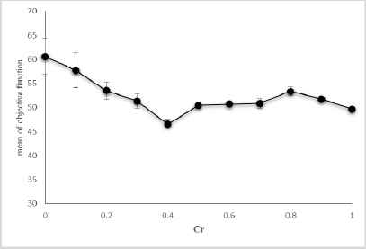
mean of objective functions and their confidence intervals of generated problems (α = 0.95)
7.3. Efficiency of proposed algorithms for Small-Scale problems
In order to evaluate the efficiency of HS and VNS in small scales, 12 problems according to what was explained in part 7.1, are generated. The data of the problems are available in the appendix.
For the problems generated in small scales, the results of algorithms are compared with the results of optimal solution using CPLEX solver. The summarized results of the comparison are displayed in Table 4., . It is worth noting that for all test problems the optimal level of credibility is considered to be equal to 0.6.
| Problems | CPLEX | VNS | GAP (%) | Basic HS | GAP (%) | improved HS | GAP (%) | ||||
|---|---|---|---|---|---|---|---|---|---|---|---|
| B | T | B | T | B | T | B | T | ||||
| P1 | 16.6 | 0.61 | 16.6 | 4.46 | 0 | 16.6 | 36.83 | 0 | 16.6 | 35.56 | 0 |
| P2 | 15.2 | 0.83 | 16.6 | 5.77 | 8.43 | 16.6 | 32.92 | 8.4 | 16.6 | 29.21 | 8.43 |
| P3 | 24.8 | 2.27 | 24.8 | 5.4 | 0 | 24.8 | 37.51 | 0 | 24.8 | 37.1 | 0 |
| P4 | 24.8 | 4.2 | 24.8 | 5.66 | 0 | 24.8 | 37.33 | 0 | 24.8 | 36.3 | 0 |
| P5 | 18.4 | 8.75 | 18.4 | 5.85 | 0 | 18.4 | 41.48 | 0 | 18.4 | 42.79 | 0 |
| P6 | 18.4 | 12.45 | 19.1 | 7.33 | 3.66 | 18.4 | 32.65 | 0 | 18.4 | 35.88 | 0 |
| P7 | 18.4 | 11.62 | 20.8 | 7.83 | 11.54 | 21.8 | 39.14 | 15.6 | 18.4 | 34.58 | 0 |
| P8 | 18.4 | 17.01 | 19.1 | 9.56 | 3.66 | 18.4 | 40.5 | 0 | 18.4 | 31.18 | 0 |
| P9 | 15.6 | 84.39 | 18.6 | 15.01 | 16.13 | 18.6 | 42.55 | 16.13 | 16.6 | 35.15 | 6.02 |
| P10 | 18.2 | 3600 | 18.5 | 9.73 | 1.62 | 18.5 | 49.17 | 1.62 | 18.4 | 51.31 | 1.09 |
| P11 | 36.2 | 3600 | 28.3 | 23.89 | 24.03 | 21.8 | 47.8 | 1.38 | 21.5 | 51.15 | 0 |
| P12 | 42.2 | 3600 | 43.47 | 13.94 | 2.88 | 48.77 | 49.71 | 13.43 | 42.22 | 57.39 | 0 |
| average | 900.3 | 9.53 | 5.99 | 40.63 | 4.715 | 39.8 | 1.25 | ||||
Comparison of the output of CPLEX solver and HS, improved HS and VNS in small size problem
In Table 4. the value of planned optimal objective function is shown by B. In this table, T indicates the running time in second. In the above table, GAP is the percentage difference of optimal planned objective function and the best planned objective function divided by the optimal rate of planed objective function. In other words, the rate of GAP is calculated via the Eq. (36).
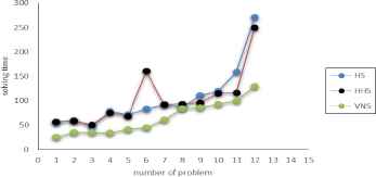
In Fig. 7. the solving time of the three algorithms are compared. In terms of solving time, basic and improved HS methods have nearly the same solving time, but in terms of solutions quality improved HS has offered better quality of solution, so that the average error percentage is 1.29% for improved HS and 4.71% for basic HS. The solving time of variable neighborhood search algorithms is relatively less than the other two algorithms but due to the lack of sufficient efficiency the average error of this algorithm is 5.99%.
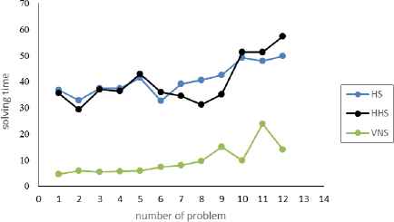
solving time of 3 algorithms for 12 problems in small sizes
The diagram of error percentage of HS and VNS is shown in Fig. 8.
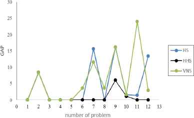
error percentage of HS, Improved and VNS algorithms
In order to examine the performance of the proposed algorithms against CPLEX solver, 8 medium size problems were generated and solved by CPLEX and presented algorithm. In all these examples, the time limit for solving by each method is considered to 3600 seconds. In Table 5. the results of numerical examples are provided with an average size.
| Problems | CPLEX | VNS | GAP | Basic HS | GAP | improved HS | GAP | |||||
|---|---|---|---|---|---|---|---|---|---|---|---|---|
| B | T | R.GAP | B | T | (%) | B | T | (%) | B | T | (%) | |
| M-P1 | 13.44 | 3600 | 0.0001 | 13.65 | 2.41 | 1.562 | 13.65 | 33.85 | 1.562 | 13.44 | 31.41 | 0 |
| M-P2 | 31.97 | 3600 | 0.002 | 31.97 | 10.79 | 0 | 31.97 | 31.21 | 0 | 31.97 | 32.39 | 0 |
| M-P3 | 91.57 | 3600 | 0.001 | 92.66 | 18.97 | 1.190 | 91.7 | 55.2 | 0.141 | 91.96 | 91.57 | 0.425 |
| M-P4 | 39.3 | 3600 | 0.009 | 39.7 | 12.6 | 0.01 | 39.3 | 37.1 | 0 | 39.3 | 40.1 | 0 |
| M-P5 | 34.1 | 3600 | 0.016 | 33.7 | 14.8 | - | 37.3 | 39.6 | - | 16.6 | 43.4 | - |
| M-P6 | 42.7 | 3600 | 0.029 | 39.6 | 15.1 | - | 38.9 | 34.2 | - | 24.8 | 42.8 | - |
| M-P7 | 49.3 | 3600 | 0.191 | 44.2 | 17.9 | - | 44.2 | 44.1 | - | 24.8 | 50.6 | - |
| M-P8 | 52.9 | 3600 | 0.206 | 49.1 | 22.6 | - | 51.6 | 49.2 | - | 18.4 | 55.2 | - |
| average | 3600 | 0.0567 | 14.396 | 0.942 | 40.557 | 0.4261 | 48.433 | 0.106 | ||||
results of median size problems
In Table 5. R.GAP is related gap that GAMS offer after 3600 seconds. The results show that in 9 examples with a median size, CPLEX solver is not able to report the optimal solution for less than 3600 seconds. Finally all algorithms used in the fourth example provided a better solution than the solver CPLEX. As respect to this matter that CPLEX cannot have a better performance than the proposed metaheuristics in median size problems, so in large scale problems we just compare our algorithms.
7.4. Efficiency of proposed algorithms for large-scale problems
In order to investigate the ability of basic HS, improved HS and VNS algorithm in large scale, 12 large scale problems have been generated and solved by metaheuristic algorithms. The data of the problems are presented in the appendix. The summary of the results are illustrated in Table 6., . It is worth noting that for all test problems the optimal level of credibility is considered to be equal to 0.6.
| problems | VNS | GAP | Basic HS | GAP | Improved HS | GAP | ||||
|---|---|---|---|---|---|---|---|---|---|---|
| B | T | (%) | B | T | (%) | B | T | (%) | ||
| B_P1 | 23.65 | 25.11 | 0 | 23.65 | 56.01 | 0 | 23.65 | 56.5 | 0 | |
| B_P2 | 63.21 | 35.14 | 6.95 | 58.85 | 60.52 | 0.05 | 58.82 | 58.26 | 0 | |
| B_P3 | 57.69 | 34.85 | 3.67 | 55.75 | 47.25 | 0.32 | 55.57 | 50.61 | 0 | |
| B_P4 | 140.68 | 34.14 | 6.83 | 138.55 | 78.39 | 5.4 | 131.07 | 75.5 | 0 | |
| B_P5 | 75.34 | 41.75 | 0 | 76.51 | 71.51 | 1.53 | 76.32 | 68.15 | 1.30 | |
| B_P6 | 150.24 | 45.18 | 0 | 156.26 | 83.14 | 3.85 | 157.52 | 160.37 | 4.62 | |
| B_P7 | 183.65 | 60.81 | 5.89 | 172.84 | 92.03 | 0 | 175.79 | 91.76 | 1.68 | |
| B_P8 | 170.18 | 84.42 | 0 | 174.65 | 86.96 | 2.56 | 174.65 | 93.42 | 2.56 | |
| B_P9 | 206.25 | 85.6 | 7.99 | 205.66 | 110.61 | 7.73 | 189.77 | 95.78 | 0 | |
| B_P10 | 224.01 | 93.32 | 7.23 | 207.81 | 119.99 | 0 | 207.81 | 115.57 | 0 | |
| B_P11 | 262.68 | 99.95 | 14.78 | 249.28 | 159.31 | 10.2 | 223.85 | 116.37 | 0 | |
| B_P12 | 247.11 | 129.36 | 0 | 273.41 | 270.76 | 9.62 | 249.61 | 249.93 | 2.20 | |
| Average | 64.1385 | 4.445 | 103.04 | 3.441 | 102.685 | 0.964 | ||||
Performance comparison of HS, improved HS and VNS algorithm in large-scale problems
The solving time for large-scale problems of basic and improved HS and VNS algorithm is displayed in Fig. 9. As it is predictable, the mean of VNS solving time is less than that of HS algorithms. The average solving time of basic HS and improved HS is 103.04 and 102.68 seconds respectively while this time for VNS algorithm is 53.54 seconds.
solving time for HS and VNS algorithm in large-scale problems
In terms of solution quality, improved HS has been able to offer the mean error of about 0.96%. This value for basic HS is about 3%. The highest rate of solution improvement for the improved HS has occurred in problems 9 and 11 and 12. Fig. 10. shows the rate of improvement by improved HS.
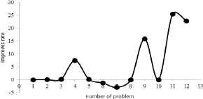
improvement through improved harmony search algorithm
Given that comparison between the metaheuristics methods, it is necessary to use nonparametric tests the performance of these algorithms [30]. To this aim the Friedman test was used in the software SPPS. Data from small, median and large-scale are analyzed by Friedman test. In the Fig. 11. output of SPSS software was showed to rank the proposed metaheuristic
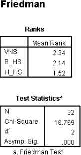
Results of Friedman test
As can be seen harmony search algorithm developed its lowest rating in terms of objectives and worked better than other algorithm. Also check the information entered in the statistical distribution of error is 0.05 times. Since asymp.sig is less than 0.05. Therefore it follows that average method used for solving the problem are introduced to one another distinction.
In terms of solution quality, HS has found better solutions than VNS algorithm in 9 cases out of 15.
8. Conclusion
In this article an uncertain integrated model of locating temporary depots in the affected areas, allocating the affected areas to these centers, and routing the required goods in such centers was introduced. The proposed model aimed to reduce the time to reach the last relief center. In order to deal with the uncertainty of the model parameters, fuzzy reliability theory and Monte Carlo simulation were applied. With regard to NP-Hard nature of the problem, a metaheuristic algorithm based on harmony search method to solve the problem is proposed. Also in order to produce initial solutions two heuristic algorithm have been proposed.
The proposed algorithm in small size problems had a better performance than basic harmony algorithm and variable search algorithm in terms of solution quality with regard to the about 1% average error and 40 seconds average time. Also the performance of improved HS in large scale was better than the other two algorithms in terms of quality according to the obtained results. In large scale problems, the average error and CPU time of VNS algorithm, basic harmony algorithm and improved algorithm respectively were 4.4% , 3.4% and 2.3% and 45, 90.4 and 89.9 seconds. The result shows the appropriate performance of improved HS. With regard to the importance of uncertainty in relief operations, considering other approaches to deal with uncertainty in the problem such as proposing a robust model for this issue is suggested for the future studies.
Appendix (A.1)
In Table 7. to Table 10., R is the total number of points and n is the number of points with demands, K is the number of vehicles, Q is the capacity of each vehicle.
| Problems | R | n | K | Q | dismax | ρ | Ba |
|---|---|---|---|---|---|---|---|
| P1 | 5 | 4 | 3 | 15 | 7 | 0.29 | 0 |
| P2 | 6 | 5 | 3 | 30 | 6 | 0.20 | 0 |
| P3 | 8 | 6 | 3 | 30 | 5 | 0.25 | 0 |
| P4 | 9 | 7 | 3 | 25 | 8 | 0.25 | 0 |
| P5 | 10 | 7 | 3 | 30 | 7 | 0.23 | 0 |
| P6 | 10 | 9 | 3 | 40 | 7 | 0.25 | 0 |
| P7 | 11 | 7 | 3 | 35 | 7 | 0.27 | 1 |
| P8 | 13 | 10 | 3 | 50 | 8 | 0.27 | 2 |
| P9 | 15 | 10 | 3 | 45 | 9 | 0.35 | 2 |
| P10 | 20 | 15 | 3 | 125 | 2 | 0.1 | 1 |
| P11 | 20 | 15 | 3 | 125 | 7 | 0.27 | 3 |
| P12 | 25 | 15 | 3 | 125 | 7 | 0.24 | 3 |
generated small test problems
| Problems | R | n | K | Q | dismax | ρ | Ba |
|---|---|---|---|---|---|---|---|
| M_P1 | 21 | 86 | 3 | 12 | 15 | 0.24 | 3 |
| M_P2 | 21 | 119 | 3 | 15 | 20 | 0.26 | 3 |
| M_P3 | 23 | 103 | 5 | 22 | 25 | 0.25 | 3 |
| M_P4 | 20 | 15 | 3 | 150 | 10 | 0.25 | 3 |
| M_P5 | 25 | 20 | 3 | 150 | 10 | 0.20 | 3 |
| M_P6 | 25 | 22 | 3 | 150 | 12 | 0.25 | 4 |
| M_P7 | 30 | 25 | 3 | 150 | 13 | 0.25 | 4 |
| M_P8 | 30 | 27 | 3 | 150 | 15 | 0.23 | 5 |
generated median test problems
| problems | R | n | K | Q | dismax | Ba |
|---|---|---|---|---|---|---|
| B_P1 | 30 | 25 | 5 | 120 | 20 | 4 |
| B_P2 | 35 | 20 | 5 | 95 | 20 | 4 |
| B_P6 | 40 | 35 | 5 | 166 | 23 | 4 |
| B_P4 | 50 | 40 | 8 | 119 | 21 | 5 |
| B_P5 | 60 | 50 | 8 | 148 | 23 | 6 |
| B_P6 | 70 | 55 | 8 | 156 | 23 | 6 |
| B_P7 | 75 | 65 | 8 | 210 | 22 | 6 |
| B_P8 | 80 | 70 | 10 | 163 | 22 | 7 |
| B_P9 | 90 | 80 | 10 | 183 | 23 | 8 |
| B_P10 | 100 | 90 | 10 | 208 | 22 | 10 |
| B_P11 | 150 | 130 | 10 | 296 | 23 | 15 |
| B_P12 | 200 | 160 | 20 | 187 | 23 | 20 |
generated large test problems
| problems | Cr | 0 | 0.1 | 0.2 | 0.3 | 0.4 | 0.5 | 0.6 | 0.7 | 0.8 | 0.9 | 1 |
|---|---|---|---|---|---|---|---|---|---|---|---|---|
| P1 | B | 16.6 | 16.6 | 16.6 | 16.6 | 16.6 | 16.6 | 16.6 | 16.6 | 16.6 | 16.6 | 16.6 |
| M | 16.6 | 16.6 | 16.6 | 16.6 | 15.5 | 16.6 | 16.6 | 16.6 | 16.6 | 16.6 | 16.6 | |
| P2 | B | 16.6 | 16.6 | 16.6 | 16.6 | 15.2 | 16.6 | 16.6 | 16.6 | 16.6 | 16.6 | 16.6 |
| M | 16.6 | 45.89 | 16.6 | 16.6 | 45.89 | 45.89 | 45.89 | 16.6 | 16.6 | 16.6 | 16.6 | |
| P3 | B | 24.8 | 24.8 | 24.8 | 24.8 | 24.8 | 24.8 | 24.8 | 24.8 | 24.8 | 24.8 | 29.7 |
| M | 74.36 | 59.09 | 54.83 | 74.36 | 25.79 | 63.08 | 25.29 | 58.39 | 74.37 | 58.97 | 29.7 | |
| P4 | B | 24.8 | 24.8 | 24.8 | 24.8 | 24.8 | 24.8 | 24.8 | 24.8 | 24.8 | 24.8 | 25.2 |
| M | 58.45 | 55.95 | 54.5 | 24.8 | 36.27 | 56.69 | 39.75 | 57.65 | 58.66 | 49.8 | 25.2 | |
| P5 | B | 18.4 | 18.4 | 18.4 | 18.4 | 18.4 | 18.4 | 18.4 | 18.4 | 18.4 | 18.4 | 18.4 |
| M | 51.3 | 50.42 | 49.49 | 49.46 | 42.21 | 55.19 | 27.66 | 49.49 | 45.58 | 18.4 | 18.4 | |
| P6 | B | 18.4 | 18.4 | 18.4 | 18.4 | 18.4 | 18.4 | 18.4 | 18.4 | 18.6 | 18.6 | 18.6 |
| M | 49.89 | 55.17 | 49.89 | 55.15 | 51.29 | 19.5 | 49.9 | 18.4 | 18.6 | 18.6 | 18.6 | |
| P7 | B | 18.4 | 18.4 | 18.4 | 18.4 | 18.4 | 18.4 | 18.4 | 18.4 | 18.4 | 18.4 | 18.4 |
| M | 18.4 | 18.4 | 50.1 | 18.4 | 18.4 | 18.4 | 18.4 | 49.85 | 18.4 | 18.4 | 18.4 | |
| P8 | B | 18.4 | 18.4 | 18.4 | 18.4 | 18.4 | 18.4 | 18.4 | 18.4 | 18.4 | 18.4 | 18.4 |
| M | 48.68 | 18.4 | 45.33 | 27.44 | 18.4 | 18.4 | 45.53 | 45.57 | 50.81 | 18.4 | 18.4 | |
| P9 | B | 15.6 | 15.6 | 15.6 | 15.6 | 15.6 | 15.6 | 15.6 | 15.6 | 15.6 | 16.5 | 16.5 |
| M | 52.4 | 52.38 | 50.89 | 52.39 | 28.11 | 52.39 | 28.19 | 34.29 | 42.57 | 16.5 | 16.5 | |
| P10 | B | 17.9 | 16.9 | 23.4 | 14.5 | 18.2 | 21.1 | 18.9 | 24.2 | 17.7 | 24.3 | 20.4 |
| M | 52.4 | 36.1 | 36 | 64.09 | 38.79 | 39.89 | 67.69 | 24.2 | 17.7 | 24.3 | 20.4 | |
| P11 | B | 58.46 | 55.95 | 54.5 | 24.8 | 36.27 | 56.7 | 39.75 | 57.65 | 58.67 | 49.8 | 25.2 |
| M | 18.4 | 18.4 | 18.4 | 18.4 | 18.4 | 18.4 | 18.4 | 18.4 | 18.4 | 18.4 | 18.4 | |
| P12 | B | 51.3 | 50.42 | 49.5 | 49.47 | 42.22 | 55.2 | 27.66 | 49.5 | 45.59 | 18.4 | 18.4 |
| M | 18.4 | 18.4 | 18.4 | 18.4 | 18.4 | 18.4 | 18.4 | 18.4 | 18.6 | 18.6 | 18.6 | |
| P13 | B | 112 | 58 | 77.5 | 78.4 | 98.3 | 100.2 | 100.6 | 121.9 | 135.6 | 213.7 | 236.1 |
| M | 152 | 138.1 | 100.6 | 98.3 | 100.2 | 105.2 | 140.4 | 140.4 | 135.6 | 213.7 | 236.1 | |
| P14 | B | 94.2 | 97.6 | 104 | 105.5 | 101 | 105.6 | 115.7 | 130.8 | 138.2 | 144.2 | 148.6 |
| M | 155.1 | 152 | 140.6 | 139.2 | 150.3 | 140.5 | 121 | 140.4 | 138.2 | 144.2 | 148.6 | |
| P15 | B | 59.9 | 59.3 | 72.3 | 79.6 | 79.7 | 86.5 | 95 | 100.8 | 123.8 | 124.6 | 124.6 |
| M | 126.3 | 130.8 | 100 | 96.5 | 89.6 | 88.3 | 97.3 | 103.5 | 129.7 | 124.6 | 124.6 | |
| average | 49.67 | 51.73 | 53.36 | 50.81 | 50.69 | 50.45 | 46.51 | 51.34 | 53.48 | 57.74 | 60.61 | |
| Lower bound | 49.67 | 51.24 | 52.48 | 49.81 | 50.2 | 49.73 | 45.43 | 49.84 | 51.63 | 54.15 | 56.89 | |
| Upper bound | 49.67 | 52.22 | 54.24 | 51.81 | 51.18 | 51.17 | 47.59 | 52.84 | 55.33 | 61.33 | 64.33 | |
optimal value for planed objective function and mean objective function for generated problems
In Table 10., the value of planned optimal objective function is shown by B and mean objective function obtained from stochastic simulation shown by M. Also the lower bound and upper bound of confidence interval of mean objective function for each Cr level is reported in the Table 10., . It is worth noting that α is set to the 0.95.
References
Cite this article
TY  - JOUR
AU  - Mahdi Alinaghian
AU  - Alireza Goli
PY  - 2017
DA  - 2017/04/20
TI  - Location, Allocation and Routing of Temporary Health Centers in Rural Areas in Crisis, Solved by Improved Harmony Search Algorithm
JO  - International Journal of Computational Intelligence Systems
SP  - 894
EP  - 913
VL  - 10
IS  - 1
SN  - 1875-6883
UR  - https://doi.org/10.2991/ijcis.2017.10.1.60
DO  - 10.2991/ijcis.2017.10.1.60
ID  - Alinaghian2017
ER  -