
A Hybrid Fuzzy Multi-hop Unequal Clustering Algorithm for Dense Wireless Sensor Networks
- DOI
- 10.2991/ijcis.2017.10.1.63How to use a DOI?
- Keywords
- Fuzzy systems; Wireless Sensor Network; Unequal clustering; Hierarchical architecture; Multi-hop transmission
- Abstract
Clustering is carried out to explore and solve power dissipation problem in wireless sensor network (WSN). Hierarchical network architecture, based on clustering, can reduce energy consumption, balance traffic load, improve scalability, and prolong network lifetime. However, clustering faces two main challenges: hotspot problem and searching for effective techniques to perform clustering. This paper introduces a fuzzy unequal clustering technique for heterogeneous dense WSNs to determine both final cluster heads and their radii. Proposed fuzzy system blends three effective parameters together which are: the distance to the base station, the density of the cluster, and the deviation of the node’s residual energy from the average network energy. Our objectives are achieving gain for network lifetime, energy distribution, and energy consumption. To evaluate the proposed algorithm, WSN clustering based routing algorithms are analyzed, simulated, and compared with obtained results. These protocols are LEACH, SEP, HEED, EEUC, and MOFCA.
- Copyright
- © 2017, the Authors. Published by Atlantis Press.
- Open Access
- This is an open access article under the CC BY-NC license (http://creativecommons.org/licences/by-nc/4.0/).
1. Introduction
Beyond the established technologies such as mobile phones and wireless local area network (WLAN), new approaches to wireless sensor networks (WSNs) are introduced for their potential applications. According to the recent continued advances in embedded systems, especially complementary metal oxide semiconductor (CMOS) technology and miniaturization techniques have resulted in the development of small-sized devices and low cost micro sensors, which it has become possible. A WSN consists of a group of distributed sensor nodes interconnected without wires. Each of the distributed sensor node typically consists of one or more computational sensing elements, a data processing unit, memory, limited storage, communication components, and a power source, which is usually a battery, as shown in Fig. 1 1.

Sensor node architecture.
Even though, sensor nodes are not very accurate and reliable individually, their distribution in large number enhances their accuracy and reliability, they have a large coverage area and longer range. WSNs have higher degree of fault tolerance than other wireless networks since a failure of one or few nodes does not affect the operation of the network. The past few decades have witnessed interest in the potential use of WSNs, that a world without it is no longer imaginable. They are easier, faster, and cheaper to deploy than wired networks or other forms of wireless networks. WSNs revolutionize the way we live and have capability for monitoring in remote and inaccessible locations, where it is not feasible to install conventional wired infrastructure 2.
According to these varieties of applications, functions, capabilities, and sensing requirements like denser level of node deployment, higher unreliability of sensor nodes, severe energy, computation, storage constraints, and expectation to operate autonomously in unattended environments, WSNs need further researches. Important aspects on the network architectures, protocols, algorithms, and design requirements in terms of network capabilities and performance, lead to impact in the operational lifetime of the whole network. In addition; energy limitation, secure communication, synchronization, data aggregation, and quality of service (QOS) are to be considered 3. Since the wireless sensor node is often placed in a hard-to-reach location, changing the battery regularly can be costly and inconvenient. An important aspect in the development of a wireless sensor node is ensuring that there is always adequate energy available to power the system, so energy conservation is the core issue in these networks. To generate a node energy model that can accurately reveal the energy consumption of sensor nodes becomes an important issue in system design and performance evaluation for WSNs 4.
A sensor dissipates power due to three operations: sensing, communicating, and data processing. More energy is required for data communication. For example, Pottie G. J. and Kaiser W. J. 5 showed that the energy cost of transmitting a 1KB message over a distance of 100 meters is approximately equivalent to the execution of 3 million CPU instructions by a 100 MIPS/W processor. Thus, there is a need for an architecture in which the transmission to a base station (BS) is as low as possible. One of the most popular solutions is to cluster the network, and then cluster heads (CHs) are selected. In a typical clustered WSN, regular nodes sense the field and send their data to the CH, then CH transmits data to the BS after aggregation. Clustering mechanisms with hierarchical structures were applied to enhance the network performance while reducing the necessary energy consumption. Clustering the nodes in WSNs has many advantages such as scalability, energy-efficiency, fault tolerance, data aggregation/fusion, increased connectivity, load balancing, collision avoidance, and reducing routing delay 6.
In this research, we present firstly a comprehensive and state-of-the-art survey on clustering approaches in WSNS. We begin with an implementation of relevant clustering algorithms then explore the merits and the drawbacks of each algorithm. The paper presents an adequate solution for unequal clustering, i.e. cluster formation, selection of CHs, and their competition radii. With the development of computational intelligence (CI), routing protocols are now based on; reinforcement learning (RL), ant colony optimization (ACO), fuzzy logic (FL), genetic algorithm (GA), and neural networks (NNs) 7. This paper focuses on the FL concept; its role in solving the unequal cluster challenges by proposing a fuzzy system to determine the final CHs and their competition radii.
The rest of the paper is organized as follows: In section (2), definitions of WSNs, clustering features, relations between AI methods and WSN, and most distinguished algorithms in this area are reviewed and presented in a general taxonomy. In section (3), we are going to introduce our proposed scenario and simulation parameters. Solution of hotspot problem is discussed. In the section (4), we will describe our system model. In the section (5), a comprehensive comparison and results discussion are shown. Finally, conclusions are drawn.
2. Literature Review
Topology management and self-organization are primary requirements in WSNs because the difficulty to access the nodes, where groups of nodes cooperate to disseminate information gathered in their vicinity to the user 8.
Communication architecture for sensor networks pertaining to all layers of the protocol stack: physical, data link, network, transport and application layers. The energy consumption model may be defined as designing and analyzing a mathematical representation of a WSN to study the effect of changing the system parameters. There are several attempts to model the energy consumption parameters:
- •
Communication power: energy consumption per second for transmitting or receiving one unit of data from node to another node or to BS.
- •
Energy for sensing: energy consumption for sensing one bit from the field.
- •
Link data rate: average flow of traffic (bits per second) between nodes.
- •
Physical layer overhead: redundancy bits in packet at physical layer.
- •
Transient power: power wasted when node changes its operating mode.
Saving communication power is more urgent in WSNs. Consequently, to extend the sensor network lifetime, it is very important to manage carefully the very scarce battery power by limiting communications. This can be done through notably efficient routing protocols that optimize energy consumption. Communication energy consumption can be due to either “useful” or “wasteful” operations. The useful energy consumption includes transmitting or receiving data messages, and processing query requests. An energy efficient approach should decrease wasteful energy consumption and utilize useful energy as sufficiently as possible.
Previous studies proved that clustering is an effective scheme in increasing the scalability and lifetime of WSNs 9. Fig. 2 depicts an application where sensors periodically transmit information to BS. It illustrates how clustering can reduce the communication overhead for both single-hop and multi-hop networks.
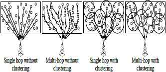
Transmission and aggregation to BS.
2.1. Taxonomy of clustering algorithms
The reviewed clustering approaches are usually classified into two major taxonomies: equal-sized and unequal-sized clustering approaches. The main idea in equal-sized clustering algorithms is to form the clusters with relatively equal sizes, keep the number of clusters as small as possible, evenly distribute them across the network, and on the other hand provide minimum overlapping among them. However, this type of clustering has a major problem: the distance between the nodes and the BS does not affect the size of clusters; consequently, the traffic load is not evenly distributed among all the nodes. Typically, in unequal clustering, the size of clusters is determined according to the distance to the BS, as the clusters are near to BS; they have to be smaller sizes. This because the closer CHs to the BS should afford intra and inter-communications more data, consequently they consume a lot of energy than the farther ones. This problem is typically known as the hotspot problem. It is better that the closer clusters to the BS be smaller. The smaller the number of cluster members, the smaller the rate of intra-cluster energy consumption. This is the basic idea behind all the unequal based approaches. Furthermore, clustering algorithms could be divided into; probabilistic and deterministic as shown in Fig. 3.

Clustering approaches classification.
Among the existing routing algorithms, LEACH is the first assumed homogeneous dynamic clustering. SEP and HEED are among most cited equal-sized clustering algorithms. On the other hand, EEUC is selected being the first algorithm that overcomes the hotspot problem. Finally, MOFCA is the most recent fuzzy based unequal-sized clustering algorithm.
2.2. Equal-sized clustering algorithms
2.2.1. Low-energy adaptive clustering hierarchy (LEACH)
LEACH 10 is the first hierarchical clustering protocol for making sensor networks energy efficient. This protocol selects CHs randomly based on predefined threshold value and then rotates this process to equilibrium the energy consumption, combines time division multiple access (TDMA) style contention-free communication with a clustering algorithm for WSNs. LEACH operates in rounds consisting of two phases: a setup phase and a steady-state phase. LEACH was introduced for prolong the network lifetime and proved to be 4 to 8 more effective than direct communication or minimum energy transfer (shortest path multi-hop routing).
From this work, three advantages for LEACH are observed: load is shared between nodes, keeps CHs away from unnecessary collisions, and avoids a lot of energy dissipation. On the other hand, LEACH has limitations such as not providing actual load balancing, using single-hop communication, non-uniform energy distribution, and finally neglecting heterogeneity factor.
2.2.2. Stable election protocol (SEP)
SEP 11 used LEACH in heterogeneous WSNs. SEP studied the impact of heterogeneity, in terms of energy of the nodes. To elect the CHs, SEP used a weighted probability method based on remaining energy in the nodes. This led to prolong the stability period of the networks. In SEP an adjustable percentage of the nodes had higher energy than the other nodes. Accordingly, a modified probability was defined to consider the residual energy. Based on this probability, the length of used epoch was increased. One of the main advantages of SEP that sensor nodes did not need any global knowledge of energy, whereas the SEP strategy still suffers from the randomization of CHs selection and its dependency on only single-hop communications, which causes the faraway nodes from BS to die faster than the nearest nodes.
2.2.3. Hybrid energy-efficient distributed clustering (HEED)
A hybrid clustering approach HEED 12, which extends LEACH by incorporating communication range limits and intra-cluster communication cost information. The initial probability for each node to become a tentative CH depends on its residual energy, and final CHs are selected according to the cost. This results in a reduction in the number of CHs in the network so the routing latency is reduced and the network lifetime is increased. In the implementation of HEED, multi-hop routing is used when CHs deliver the data to BS. However, the authors have not considered the hotspot problem when multi-hop forwarding model is adopted. HEED is a fully distributed cluster-based routing technique that achieves load balancing, uniform CH distribution, high-energy efficiency, and scalability. On the other hand, the CHs that were created by HEED, generate massive overhead, and estimates large iterations than necessary.
2.3. Unequal-sized clustering algorithms
2.3.1. Unequal clustering scheme (UCS)
In UCS 13 the size of clusters is determined based on their distance to the BS, but the design of network is predefined by assuming, a BS in the middle of a circular shaped sense area, each CH has unlimited energy capability, and is located in center of its cluster. The preset clusters in the same form have the same size and the CHs send the data to the BS via a two-hop path. The main advantages rather than the equal-sized clusters, UCS achieves a load balance among the clusters, prolongs the network lifetime compared to equal-sized clustering. However, the preset clustering method is unpractical and difficult to be implemented in real applications.
2.3.2. Probabilistic unequal-sized clustering algorithms
One of the major algorithms in this area is Energy-Efficient Unequal Clustering protocol (EEUC) 14, where an unequal clustering was proposed according to the distance to the BS. In EEUC, the closer clusters to the BS are smaller than the farther ones. In addition, the CHs are elected based on a competition. First, some tentative CHs are elected from the regular nodes with a specific probability. In order to save more energy, the nodes that fail to be the tentative CHs, stay in a sleep mode until the CH election process finishes. Different competition ranges are used in order to achieve unequal clustering. A tentative CH is elected as final CH, only if it has greater residual energy than other nodes in its competition range. However, EEUC has some drawbacks: firstly, EEUC algorithm is a probabilistic clustering algorithm, which is considered insufficient selection criteria and causes in not appropriate final CH. Secondly, defining the optimum value of some parameters is not easy, especially in large-scale WSNs. Finally, broadcasting the beacon messages by the CHs results in more energy consumption than conventional shortest path multi-hop approaches.
2.3.3. Deterministic unequal-sized clustering algorithms
Unlike probabilistic unequal clustering algorithms, some approaches use more confident metrics to elect the CHs. Usually, these metrics are achieved locally based upon node conditions. The most conventional metrics in CH election are the residual energy, proximity (to neighbors/ BS), node degree (the number of neighbors in cluster range) and node centrality. These methods are called deterministic clustering algorithms, due to the criteria of elected CHs, and consequently, the formed unequal clusters are more controllable.
2.3.4. Fuzzy unequal clustering algorithms
In this section, the most important approaches in the area of the unequal clustering are based on fuzzy-logic, which requires low computation capabilities, and is able to support decision-making processes to improve efficiency and prolong the overall network lifetime. Diverse approaches using fuzzy-logic presented improvement in unequal cluster-based routing, and endorsed the use of fuzzy logic in WSNs. These approaches introduced efficient routing, since WSNs need simple and fast methods to make decisions, fuzzy logic appears as an appropriate method due to its ability to calculate results fast and precisely in a user-friendly way. In order to improve the efficiency and accuracy of the route creation process and to speed it up, evaluation of node conditions through fuzzy logic is required 15. The execution of a fuzzy logic system requires less computational power than conventional mathematical computational methods.
2.3.5. Energy aware fuzzy unequal clustering (EAUCF)
An unequal clustering algorithm based on fuzzy logic is proposed to determine the cluster size according to the vicinity to the BS and node remaining energy. The highest residual energy within the competition range is an essential factor for determining CHs; then, the non-CH nodes join with the CH close to them. Although, EAUCF is a stable and energy-efficient clustering algorithm to be utilized in any real time WSN application. EAUCF suffers from the energy depletion at the CH 16.
2.3.6. Multi-objective fuzzy clustering algorithm (MOFCA)
In similar to EAUCF a fuzzy-based proposed to generate the unequal clusters was introduced to adjust the CH competition radius according to three parameters: remaining energy, distance to BS, and density of the nodes. First, each node produces a random number between zero and one then compares it to a predefined threshold (T). If the node finds its number less than T, it elects itself as a tentative CH. Then, the tentative CHs with higher residual energy are elected as the final CHs. The competition radius of each tentative CH changes dynamically according to fuzzy system output. MOFCA did not work with a central decision node (BS) for electing process. On the other hand, a few drawbacks could be observed: nodes in dense area may have large probability to become CH (wrong decision), neglecting of the first radio model, and finally rounds could end without appropriate CH election 17.
3. Proposed Fuzzy Unequal Clustering Model
The purpose of our methodology is to minimize the overall energy dissipation in the network, extend network lifetime, and overcome the hotspot problem based on a proposed fuzzy system to determine CHs and generate unequal clustering. The energy consumption of CHs is high because of receiving sensed data from their member nodes, performing data aggregation, and sending the aggregated data to the next hop node or BS. Therefore, the operation of clustering protocols is divided into rounds and the role of the CH must be rotated among all sensor nodes within these rounds.
3.1. Proposed model assumptions
In our scenario, some assumptions are proposed for sensor nodes, radio model, and the underlying network model:
- (i)
A single Base station is fixed, immobile, and has unlimited resources.
- (ii)
All the nodes are assumed to be energy constrained in nature.
- (iii)
Operation of algorithm is broken into rounds, and each round has a set-up phase and a steady state phase.
- (iv)
A sensor network consists of N sensor nodes uniformly deployed over a vast field to monitor continuously the environment.
- (v)
Radio characteristics
- •
Energy loss due to channel transmission according to first order radio model.
- •
Radio channel is symmetric.
- •
An ideal MAC layer and error-free communication links.
- •
- (vi)
Sensors Characteristics
- •
Sense environments at a fixed rate or no mobility.
- •
Communicate among each other and to the BS.
- •
Deploy in random and non-deterministic manner in a large-scale area.
- •
Send location information and energy level to BS during set up phase.
- •
Capable of adjusting the amount of transmission power according to the distance.
- •
- (vii)
The delay of the broadcast process and the calculation process is negligible.
3.2. Proposed fuzzy system
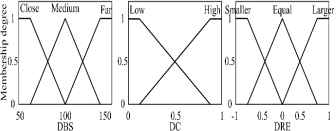
The proposed hybrid fuzzy multi-hop unequal clustering (HFMUC) determines the probability of node to be a CH based on a local decision. Moreover, it generates tentative CHs and their competition radii based on the same fuzzy system. This fuzzy system considers three inputs; distance to the BS (DBS), density of the cluster (DC), and deviation of node’s residual energy from the average network energy (DRE). The system has two outputs: CH probability (CHprob) and the competition radius for tentative CHs (Rcomp).
The fuzzy sets, defining the input variable, are depicted in Fig. 4. The second fuzzy input variable is the DC, which is estimated by Eq. (1).
Proposed membership functions for input variables.
Since the number of alive nodes may change at the start of each round and it is not possible for the node to know this value, so the BS should broadcast this value at the start of every round.
The third fuzzy input variable is DRE. To estimate the value of DRE, first the average energy of the entire network (avg) at each start of a new round is calculated as Eq. 2.
The result of Eq. 3 could be zero, positive or negative.
The fuzzy rules are given in Table 1. In order to evaluate the rules, the Mamdani Controller is used as a fuzzy inference technique and the center of area (COA) method is employed for defuzzification of both CHprob and Rcomp, based on the three fuzzy input variables (descriptors), are used. The first fuzzy set output variable is referring to CHprob has three linguistic variables, which are small probability (S.Prob), Medium probability (M.Prob), and high probability (H.Prob). Where M.Prob has a triangular membership function while S.Prob, and H.Prob are both represented by trapezoidal membership functions. The second fuzzy set output variable refers to the Rcomp that has 18 linguistic variables, which are 8XS (extra small) to 8XL (extra-large). The 8XS and 8XL are represented by trapezoidal membership functions and the remaining linguistic variables have triangular membership functions.
| DBS | DC | DRE | CHprob | Rcomp |
|---|---|---|---|---|
| Close | Low | Smaller | S.Prob | 8XS |
| Close | Low | Equal | M.Prob | 7XS |
| Close | Low | Larger | H.Prob | 6XS |
| Close | High | Smaller | S.Prob | 5XS |
| Close | High | Equal | M.Prob | 4XS |
| Close | High | Larger | H.Prob | 3XS |
| Medium | Low | Smaller | S.Prob | 2XS |
| Medium | Low | Equal | M.Prob | XS |
| Medium | Low | Larger | H.Prob | S |
| Medium | High | Smaller | S.Prob | L |
| Medium | High | Equal | M.Prob | XL |
| Medium | High | Larger | H.Prob | 2XL |
| Far | Low | Smaller | S.Prob | 3XL |
| Far | Low | Equal | M.Prob | 4XL |
| Far | Low | Larger | H.Prob | 5XL |
| Far | High | Smaller | S.Prob | 6XL |
| Far | High | Equal | M.Prob | 7XL |
| Far | High | Larger | H.Prob | 8XL |
HFMUC Fuzzy rules.
3.3. HFMUC operations flow
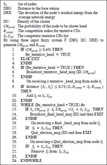
The pseudo-code of the proposed algorithm is shown in Fig. 5; the operation of the proposed HFMUC protocol is described as follows:
- •
Set-up phase
- (i)
At the beginning of each round: the BS broadcasts a “hello” message periodically with a certain given power level that covers the entire network and contains the network average energy and the total number of alive nodes.
- (ii)
Each node computes the approximate distance to the BS (DBS) and the value of DRE.
- (iii)
Each node receives the messages from all neighbors in its radio range then computes the distances to its neighbors and the density of the nodes on its radio range (DC).
- (iv)
The proposed fuzzy system generates CHprob and Rcomp and satisfies line 1 in the pseudo code if (CHprob ≥ 0.49) nodes is elected as a tentative CH.
- (v)
Now each node has to update its neighborhood table to store the information about its neighbors.
- (vi)
Line 9 in the pseudo code is satisfying the competition tentative CHs condition. Where candidate CHs are considered as a competitor-tentative CHs only if the distance between them is less than a 0.75 of the summation of their radii to improve the coverage for the entire network and guarantee minimum overlapping area. Also, that condition guarantees the optimum selection of final CHs, this is illustrated in Fig. 6 where n1, n2, n3, and n4 are all a tentative CHs, but n1 and n4 are only the competitor-tentative CHs.
- (vii)
The while loop in line 12 of the pseudo code, determines the final CH.
- (viii)
The competitor-tentative CH announces itself as final CH if it has the largest CHprob in all the competitor-tentative CH list, or quit the election and considering itself “covered” if it has heard a final CH announcement. Otherwise, it updates its status and the competitor-tentative CH list until being a final CH or a normal node.
- (i)
- •
Steady-state phase
- (i)
Each non-CH node receives advertisements from the nearest CHs. Node selects the cluster to join based on the largest received signal strength indication (RSSI).
- (ii)
Each CH assigns a TDMA schedule.
- (iii)
Each CH waits to receive data from all nodes in its cluster and then compresses and sends the aggregated result back to the BS or to the nearest CH, which is close to BS according to the threshold distance, which in turn is determined by the first radio model as shown in Fig. 7, then algorithm is repeated.
- (i)
HFMUC pseudo-code.
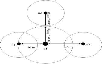
Tentative CH list competition.

Multi-Hop communication flowchart.
4. Results and Discussion
4.1. Scenarios and parameters description
Simulation starts with implementation of some surveyed algorithms: LEACH – SEP – HEED – EEUC - MOFCA. This implementation is necessary for results discussion and comparisons. The i-th sensor is denoted by si and the corresponding sensor node set S where |S|= N. Simulation parameters are given in the following Table 2.
| Parameters | Definition | Unit Values |
|---|---|---|
| rmax | Simulation rounds | 1500 rounds |
| x * y | Network area size | 100 * 100 m2 |
| N | Number of nodes | 200 nodes |
| BS | Number of gateway nodes | 1 BS |
| BS location | Location from area of the interest (AOI) | 1.5x * 0.5y |
| m | Heterogeneity percentage rate | 20% |
| α | Exceeded value of advanced nodes | 1 |
| Eo | Initial node power | 0.5 Joule |
| ETX | Energy for transmission | 50 nJ/bit |
| ERX | Energy for reception | 50 nJ/bit |
| EDA | Energy for data aggregation | 5 nJ/bit |
| Eelec | Circuitry dissipation | ETx-elec = ERx-elec |
| Eamp | Transmit amplifier | εfs OR εmp |
| εfs | Energy dissipation at free space | 10 pJ/ bit /m2 |
| εmp | Energy for multi-path fading | 0.0013 pJ/ bit /m4 |
| do | Threshold distance
|
87.7m |
| K | Data packet size | 500 byte |
| l | Broadcast packet size | 20 byte |
| Cr | Radio range of CH | 50m |
Summary of parameter values.
The first order radio model is taken into consideration when deducting transmission and reception power dissipated in communication. In order to achieve an acceptable Signal-to-Noise Ratio (SNR) in transmitting a K−bit message over a distance d, the energy expended by the radio model is given by Eq. 4 and Eq. 5:
Then to receive this message, the radio expends:
4.2. Performance measures
There are a lot of metrics to evaluate the performance of the clustering protocols 1, in this research, two new metrics are introduced which are rate of energy consumption and energy level of first dead node:
- •
Network lifetime: The total number of round from the start of the operation of a WSN until the death of the last alive sensor.
- •
Stability period: The number of rounds from the start of a WSN operation until the death of the first sensor.
- •
First dead node (FDN): Number of rounds when the first sensor dies. This parameter has a direct relation with the stability period parameter. Where, the highest FDN indicates the longer stability period of network.
- •
Half dead node (HDN): Number of rounds when half the number of sensor nodes is dead.
- •
Last dead node (LDN): Number of rounds when all sensor nodes are dead.
- •
Number of alive nodes per round: This instantaneous measure reflects the number of nodes that have not yet expended their total amount of energy.
- •
Rate of energy consumption (REC): The rate of change in energy consumption per round within stability period.
- •
Energy level at FDN (ELFND): The Average remaining energy of network when the first sensor dies. This parameter has direct relation with energy distribution parameter, i.e. the lowest ELFDN is the better energy distribution.
4.3. Stability period discussion
It is clear that the larger stability period is better in calibrating the reliability of WSN, while the traditional definition of stability period is the number of rounds from the start of a WSN operation to the death of the first sensor. However, for experimental measurements in our simulation, the entire network works until the most of sensor nodes are dead. The LDN metric should not be considered, since the WSNs are useless after half of the total nodes die. Instead of caring about the LDN, new aspects will be introduced, which are the second and the third dead nodes that may change the definition of the stability period. Fig. 8 shows the simulation results of the number of alive nodes per round for the proposed method HFMUC with other simulated algorithms LEACH, SEP, HEED, HEED with multi-hop (MHEED), EEUC, and MOFCA.
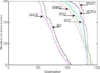
Number of alive nodes per round.
Table 3 is concluded from the previous figure. It indicates the FDN, the second dead node (2ndDN), the third dead node (3rdND), and HDN of each algorithm. Furthermore, it clarifies the new proposed definition for the stability period observation in terms of percentage node failure. It also turns out that HMFUC has the longest stability period compared with all implemented algorithms.
| Algorithm | FDN | 2ndDN | 3rdND | HDN |
|---|---|---|---|---|
| LEACH | 515 | 522 | 523 | 804 |
| SEP | 578 | 584 | 584 | 846 |
| HEED | 732 | 746 | 753 | 1274 |
| MHEED | 864 | 900 | 906 | 1299 |
| EEUC | 951 | 987 | 995 | 1309 |
| MOFCA | 1024 | 1041 | 1076 | 1307 |
| HFMUC | 1201 | 1202 | 1202 | 1341 |
Stability period comparison between simulated algorithms.
Table 4 indicates the percentage of gain in the stability of HFMUC over the six introduced algorithms, which is calculated by Eq. 6
| Algorithm | % of the gain in stability period of HFMUC over other algorithms |
|---|---|
| LEACH | 133% |
| SEP | 108% |
| HEED | 64% |
| MHEED | 39% |
| EEUC | 26% |
| MOFCA | 17% |
Percentage of gain in stability period when using HFMUC vs other techniques.
From this table, it is clear that HMFUC exceeds all the compared algorithms in different percentages, which clarifies that the new proposed algorithm has given an advantage than LEACH, SEP, HEED, EEUC, and MOFCA through its stability period.
4.4. Energy evaluation
Fig. 9 shows the average of the total remaining energy until the FDN per round for each algorithm. From this figure, we noticed that the total remaining energy curve is linear until FDN (stability period). In addition, we concluded that HFMUC surpasses all the implemented protocols by its linearity with the lowest slope, also the lowest remaining energy at FDN, which is referring to better energy distribution.
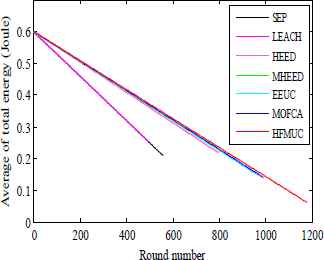
Average of the entire remaining energy until FDN per round.
As shown in Table 5, ELFDN is presented by the average of the remaining energy of the entire network at FDN for each protocol. Where the slopes of the curves - obtained from Fig. 9- represent the rate of energy consumption per round (REC) within the interval of stability period, the slope of each curve is calculated by using the summation of the differences between nodes energies divided over the total number of differences. Then the percentage of uniform energy sustainability is calculated by deducting the percentage of the average remaining energy when first sensor dies (ELFDN) from the overall average energy. We found that HFMUC has the least REC, which is effective for balancing energy consumption and saving node energy.
| Algorithm | ELFDN (Joule) | REC (µJoule / round) | Percentage of uniform energy sustainability |
|---|---|---|---|
| LEACH | 0.252 | 696.75 | 58% |
| SEP | 0.211 | 698.24 | 64.8% |
| HEED | 0.218 | 478.57 | 63.7% |
| MHEED | 0.245 | 463.56 | 59.2% |
| EEUC | 0.146 | 467.16 | 75.7% |
| MOFCA | 0.140 | 463.40 | 76.7% |
| HFMUC | 0.0623 | 456.44 | 89.6% |
Comparing energy consumption and distribution within stability period.
4.5. Impact of HFMUC overhead communication
The total energy dissipation of the network is divided into the data-energy consumption and the overhead-energy consumption, Fig. 10 illustrates both consumptions for each algorithm within the stability period.
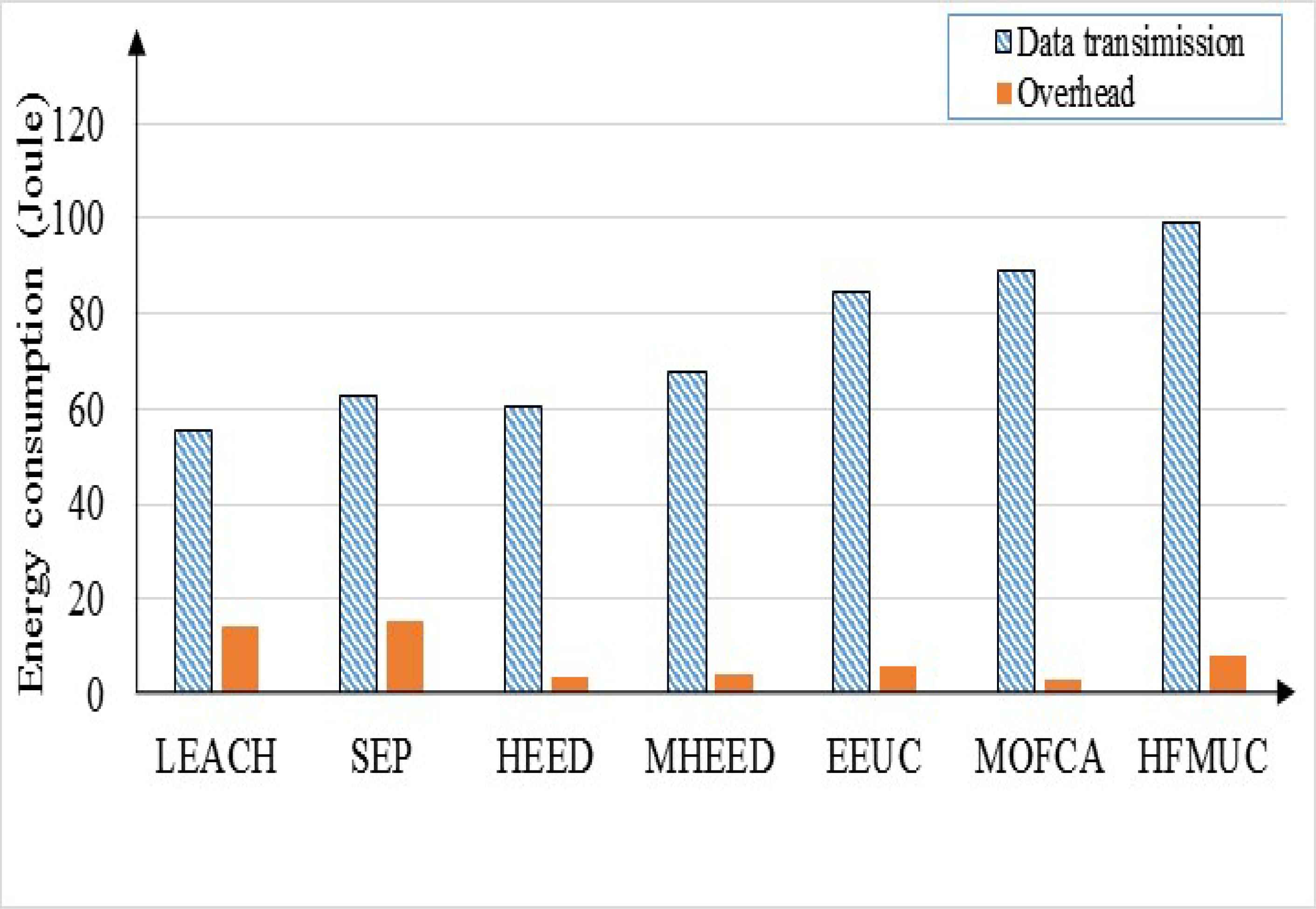
Energy consumption of overhead vs data transmission.
Table 6 indicates the values of the data-energy consumption and the overhead-energy consumption for each algorithm until FDN. It is clear, that energy consumption of the overhead communication in HFMUC is moderate, and also the energy dissipated in transmission data is better than the other algorithms, due to the long stability period of HFMUC.
| Algorithm | Data energy consump. (Joule) | Overhead consump. (Joule) | Percentage of overhead consumption |
|---|---|---|---|
| LEACH | 55.5 | 14.1 | 20% |
| SEP | 62.5 | 15.3 | 19.5 |
| HEED | 60.5 | 3.5 | 5.46% |
| MHEED | 68 | 4 | 5.5% |
| EEUC | 84.6 | 6.1 | 6.7% |
| MOFCA | 88.8 | 3.3 | 3.6% |
| HFMUC | 99 | 8 | 7.4% |
Percentage of overhead energy consumption.
From simulation results, it is clear that the proposed HFMUC surpasses all benchmark methods in: longer stability period, less energy consumption, and better energy distribution. However, the proposed method adds more overhead messages between tentative CHs during the competition when compared to HEED, MHEED, EEUC, and MOFCA. Further researches are to be considered to decrease the size of such messages.
5. Conclusion
This paper has introduced an HFMUC technique that organized sensor nodes into unequal clusters communicating in multi-hop manner. Through this work, two new metrics were defined as the rate of energy consumption and energy level of the first dead node. Five state-of-the-art algorithms were simulated to compare our proposed HFMUC. From this simulation, it was found that HFMUC has given 17% to 133% better stability period compared to MOFCA and LEACH respectively. Furthermore, the uniform energy sustainability was 89.6% compared to 76.7% for MOFCA, and to 58% for LEACH. Our objectives in improving network lifetime, energy distribution, and energy consumption are achieved. This proves that our method fits better with real time applications and emergent event monitor.
References
Cite this article
TY  - JOUR
AU  - Shawkat K. Guirguis
AU  - Mohamed A. Abdou
AU  - Ahmed A. Elnaggar
PY  - 2017
DA  - 2017/05/18
TI  - A Hybrid Fuzzy Multi-hop Unequal Clustering Algorithm for Dense Wireless Sensor Networks
JO  - International Journal of Computational Intelligence Systems
SP  - 951
EP  - 961
VL  - 10
IS  - 1
SN  - 1875-6883
UR  - https://doi.org/10.2991/ijcis.2017.10.1.63
DO  - 10.2991/ijcis.2017.10.1.63
ID  - Guirguis2017
ER  -