
Generalizing linguistic distributions in hesitant decision context
- DOI
- 10.2991/ijcis.2017.10.1.65How to use a DOI?
- Keywords
- decision making; computing with words; hesitant fuzzy linguistic term set; linguistic distribution
- Abstract
The hesitant fuzzy linguistic term set (HFLTS) and the linguistic distribution (LD) are becoming popular tools to describe decision makers’ linguistic preferences. By combining HFLTS and LD, this paper proposes a new concept called hesitant linguistic distribution (HLD), and then presents the transformation between HLDs and LDs and the basic comparison and aggregation operations to perform on HLDs. Following, comparisons among several linguistic expressions are made. Finally, the use and behavior mechanism of HLD in multiple attribute group decision making is demonstrated.
- Copyright
- © 2017, the Authors. Published by Atlantis Press.
- Open Access
- This is an open access article under the CC BY-NC license (http://creativecommons.org/licences/by-nc/4.0/).
1. Introduction
Linguistic decision making in which linguistic information is utilized to describe decision makers’ preferences/opinions qualitatively is a common activity in our daily life, and different linguistic approaches have been proposed to deal with computing with words (CW) [11, 16, 19, 26, 36] in linguistic decision making problems. The two classical linguistic computation models: (1) the semantic model [26] and (2) the symbolic model [20, 21] have been intensively studied. Especially, the 2-tuple linguistic representation model [13], which avoids the computation weakness in information loss, has been widely applied (e.g., [4, 17, 22, 23, 24]. Furthermore, different progress has been made based on the 2-tuple linguistic model, such as the linguistic hierarchy model [12, 14], multi-granular linguistic model [25, 27], the proportional 2-tuple linguistic model [32] and the numerical scale model [5, 9].
In the above mentioned models, decision makers can only utilize single linguistic terms to elicit their preferences, which restricts decision makers from expressing their opinions with flexible and rich linguistic expressions [15, 30]. To address this issue, Rodríguez et al. [31] introduced the concept of hesitant fuzzy linguistic term set (HFLTS) taking decision makers’ hesitancy among different linguistic terms into consideration. Based on the use of HFLTS, Beg and Rashid [1] proposed a TOPSIS method to aggregate HFLTSs in multi-criteria decision making. Liu and Rodríguez [18] proposed the fuzzy envelope to carry out the CW processes of HFLTSs. Wei et al. [33] introduced the aggregation operators and comparisons of HFLTSs. Dong et al. [3] presented a novel approach to deal with consensus reaching process with hesitant linguistic assessments in group decision making. The recent progress of the HFLTS in decision making can be found in the position paper (see Rodríguez et al. [29]).
Different from the HFLTS which does not consider the symbolic proportion information of the terms, Zhang et al. [39] proposed the linguistic distribution (LD) in which symbolic proportions are assigned to all the terms in a linguistic term set. Dong et al. [7] introduced the unbalanced LD with interval symbolic proportions in multi-granular context. Wu and Xu [34] proposed the possibility distributions for HFLTS with symbolic proportions uniformly distributed over the terms in an HFLTS. Chen et al. [2] proposed the proportional hesitant fuzzy linguistic term set which includes the proportional information of generalized linguistic terms. Zhang et al. [41] discussed the LDs in large-scale multi-attribute group decision making (MAGDM). Pang et al. [28], Guo et al. [10] and Wu and Dong [35] discussed the cases of LDs with incomplete information.
However, in the LD and its variants, all symbolic proportion information of these expressions are focused on single terms, and in some situations decision makers have to express symbolic proportion information over HFLTSs. For example, an expert is asked to evaluate on a football player according to the player’s past performances. The established linguistic term set is S = {s0 : very poor, s1 : poor, s2 : slightly poor, s3 : medium, s4 : slightly good, s5 : good, s6 : very good}.
When evaluating, the expert considers that the proportion of the performance ‘good’ is 0.3, the performance ‘slightly good’ is 0.2 and the performance ‘very good’ is 0.2. But the expert hesitates among the terms ‘very poor’, ‘poor’, and ‘slightly poor’ and ‘medium’ and he/she could just be sure that the proportion of the performance ‘no better than medium’ is 0.3. In this situation, the evaluation provided by the expert can be described by {({s0, s1, s2, s3}, 0.3), (s4, 0.3), (s5, 0.2), (s6, 0.2)}, and the expert doesn’t provide the proportion information for single terms in {s0, s1, s2, s3} but a sum proportion for the HFLTS {s0, s1, s2, s3}. In this paper, we call this kind of evaluation information hesitant linguistic distribution (HLD). We will present the basic operations including the comparison and aggregation operations to perform on HLDs, and will also propose the comparisons among several linguistic expressions to show that the HLD is their generalization.
The rest of this paper is organized as follows. Section 2 introduces the basic knowledge regarding the 2-tuple linguistic model, HFLTS, and LD. Then, Section 3 proposes the HLD and its basic operations. Next, Section 4 presents the comparisons among several linguistic expressions. Following, in Section 5 we discuss the use and behavior mechanism of HLD in multi-attribute decision making (MAGDM). Finally, conclusion remarks are included in Section 6.
2. Preliminaries
This section introduces the basic knowledge regarding the 2-tuple linguistic model, HFLTS and LD. The introduction of the 2-tuple linguistic model is very necessary because (1) it provides the basis for CW in this paper, and (2) HFLTS and LD are both its generalization.
2.1. The 2-tuple linguistic model
Let S = {s0, s1,…, sg} be a linguistic term set with odd cardinality satisfying [11, 13, 19]:
- (1)
The set is ordered: sk ≥ st if k ≥ t ;
- (2)
There is a negation operator: neg(sk) = si such that k + t = g.
g + 1 is called the cardinality of S and the term sk (k = 0, 1, …, g) represents a possible value for a linguistic variable. The basic notations and operation laws of linguistic variables are introduced in [37].
Herrera and Martínez [13] proposed the 2-tuple linguistic model.
Definition 1 [13]:
Let S = {s0, s1,…, sg} be as before and α ∈ [0, g] be a value representing the result of a symbolic aggregation operation. A linguistic 2-tuple (sk, β) that expresses the equivalent information to α is obtained by the function:
Clearly, Δ is a one to one mapping function and the inverse function of Δ is:
For any linguistic 2-tuple of
- (1)
Negation operation:
Neg(sk, β) = Δ(g−(Δ−1(sk, β))).
- (2)
Comparison operation:
Let (sk, β1) and (st, β2) be two linguistic 2-tuples.
- (i)
If k < t, then (sk, β1) is smaller than (st, β2);
- (ii)
If k = t,
- (a)
β1 = β2, then (sk, β1) and (st, β2) represent the same information;
- (b)
β1 < β2, then (sk, β1) is smaller than (st, β2).
- (a)
- (i)
Several aggregation operators such as the linguistic weighted average (WA) operator and the ordered weighted average (OWA) operator have been developed (see [13, 20, 21]).
2.2. Hesitant fuzzy linguistic term set
The 2-tuple linguistic model proposed by Herrera and Martínez [13] can deal with linguistic information with single terms. However, there are situations that single terms cannot handle. For example, the coach may hesitate among several terms when he/she is not sure whether the performance of the player is ‘slightly good’ or ‘good’ or ‘very good’. To overcome the limitations, Rodríguez et al. [31] proposed the concept of HFLTS in which multiple consecutive terms are allowed to represent a decision maker’s hesitant preference. The concepts of HFLTS and its envelope are introduced as Definitions 2 and 4.
Definition 2 [31]:
Let S = {s0, s1,…, sg} be a linguistic term set, and an HFLTS, denoted as HS, is an ordered finite subset of the consecutive linguistic terms of S.
If HS = {}, HS is called an empty HFLTS; if HS = S, HS is called a full HFLTS.
Definition 3 [31]:
Let S = {s0, s1,…, sg} be a linguistic term set, and let HS be an HFLTS. The upper bound HS+ and lower bound HS− of HS are defined as:
- (1)
HS+ = max(sk) = sj, sk ∈ HS and sk ≤ sj ∀ k;
- (2)
HS− = min(sk) = sj, sk ∈ HS and sk ≥ sj ∀ k.
Definition 4 [31]:
Let S = {s0, s1,…, sg} be a linguistic term set, and the envelope of the HFLTS, env(HS), is a linguistic interval whose limits are obtained by the upper bound (max) and lower bound (min). Hence
For any two HFLTSs
- (1)
- (2)
The details for the HFLTS can be found in Rodríguez et al. [31].
2.3. Linguistic distribution
Zhang et al. [39] and Dong et al. [7] proposed the concept of linguistic distribution, as Definition 5.
Definition 5 [7, 39]:
Let S = {s0, s1,…, sg} be a linguistic term set. Let m = {(sk, β(sk))| k = 0, 1, …, g}, where β(sk) is the symbolic proportion of sk, β(sk) ≥ 0, and
Let m = {(sk, β(sk))| k = 0, 1, …, g} be an LD over S. Then the expectation of m is defined as [7, 39]:
For any LD over S, there are the following operations:
- (1)
Negation operation:
Neg({(sk, β(sk))}) = {(sk, β(sg−k))}, k = 0,1,…, g.
- (2)
Comparison operation:
Let m1 and m2 be two LDs over S.
- (i)
If E(m1) < E(m2), m1 is smaller than m2;
- (ii)
If E(m1) = E(m2), m1 and m2 have the same expectation. Zhang et al. [41] discussed the situation when E(m1) = E(m2).
- (i)
The weighted average operator and the ordered weighted average operator of LD have been developed (see [7, 39]).
In Wu and Dong [35], LD was generalized to incomplete linguistic distribution as Definition 6.
Definition 6 [35]:
Let S = {s0, s1,…, sg} be a linguistic term set. Let m = {(sk, β(sk))| k = 0, 1, …, g}, where β(sk) ∈ [0,1]∪{null}. Then
- (1)
If β(sk) ∈ [0,1] ∀sk ∈ S and
- (2)
If there exists β(sk) = null and
The possibility distribution for HFLTS proposed in Wu and Xu [34], in which the sum of the symbolic proportions of an HFLTS of S equals to one, is a special CLD.
3. The hesitant linguistic distribution and its operations
The symbolic proportion information of LDs are over simple terms. However, in some situations, decision makers cannot provide symbolic proportion information for simple terms. Instead, they may hesitant among several consecutive terms and provide a sum of proportions for an HFLTS. In order to deal with this situation, in this section we propose the concept of hesitant linguistic distribution (HLD) and some of its operations.
3.1. Definition of the hesitant linguistic distribution
Let S = {s0, s1,…, sg} be a linguistic term set, and let HS be an HFLTS of S. Then the set of all HFLTSs of S is denoted as H in this paper.
The concept of the HLD can be formally defined as Definition 7.
Definition 7:
Let S = {s0, s1,…, sg} and H be as before, the HLD is defined as:
Further, we consider two cases:
- (1)
If
The normalized M denoted as MN is a complete hesitant linguistic distribution (CHLD) over S.
- (2)
If
Example 1.
Let S = {s0, s1, s2, s3, s4, s5, s6} be a linguistic term set. Then the set of all HFLTSs of S is:
As
3.2. The transformation and comparison operations
After introducing the concept of the HLD, it is necessary to introduce its operations. First, we propose a transformation approach between LD and HLD. Let
The transformation approach between LD and HLD can be formally presented as Algorithm I.
Algorithm I.
Input: The HLD
Output: The transformed LD M* = {(sk, αk)|k = 0,1,…, g}.
Step 1: Let αk = 0 and βk = −1 (k = 0,1,…, g).
Step 2: Let
Step 3: If H ≠ null, go to Step 2; otherwise, if βk = −1, then let αk = null. Let M* = {(sk, αk)|k = 0,1,…, g} and output M*.
We call M* the transformed LD of M.
Next, we present an example to illustrate the transformation between LD and HLD.
Example 2.
Continuing Example 1. Based on Algorithm I, the CHLD
Proposition 1:
Let
- (1)
if
- (2)
if
Proof.
Let
This completes the proof of Proposition 1.
Proposition 1 indicates that based on Algorithm I the HLD
Next, we define the comparison operations of any two HLDs based on the use of expectation and variation of transformed LD.
Definition 8:
Let M and M* = {(sk, β(sk))|k = 0,1,…, g} be as before. Then the expectation and variation of M are defined as Eqs. (4) and (5):
Let M1 and M2 be two HLDs over S, and the comparison operations between M1 and M2 are as follows.
- (1)
If E(M1) < E(M2), then M1 < M2;
- (2)
If E(M1) > E(M2), then M1 > M2;
- (3)
If E(M1) = E(M2), then
- (i)
If V(M1) < V(M2), then M1 > M2;
- (ii)
If V(M1) > V(M2), then M1 < M2;
- (iii)
If V(M1) = V(M2), then there is no difference between M1 and M2.
- (i)
Next, we present an example to illustrate the comparison operations.
Example 3.
Continuing Example 2. As E(M1) = 3.4 > E(M2) = 2.45, we have M1 > M2.
3.3. Aggregation operations for HLDs
In this section, we introduce the weighted average operator and the ordered weighted average operator for HLDs.
For any two HLDs, the weighted union of them is defined as Definition 9.
Definition 9:
Let S = {s0, s1,…, sg} and H be as before, and let
Example 4.
Continuing Example 2. Suppose the weights for M1 and M2 are w1 = 0.6 and w2 = 0.4. Then
Based on Definition 9, we introduce the weighted average operator and the ordered weighted average operator for HLDs as Definitions 10 and 11.
Definition 10:
Let S = {s0, s1,…, sg} and H be as before, and let {M1, M2,…, Mn} be a set of HLDs over S, where
Definition 11:
Let S = {s0, s1,…, sg} and H be as before, and let {M1, M2,…, Mn} be a set of HLDs over S, where
Example 5:
Continuing examples 1–3. Let {M1, M2, M3, M4, M5} be a set of HLDs over S, where M3, M4 and M5 are as follows:
Without loss of generality, assume that w = (0.2,0.3,0.2,0.2,0.1)T. Then
Based on Definition 8, we have:
So,
Following, we discuss the desirable properties of the proposed operators. We take the ordered weighted average operator as example, and the properties of the weighted average operator are similar with the ordered weighted average operator.
Property 1.
Let {M1, M2,…, Mn} and w = {w1, w2,…, wn}T be as before. For any HLDOWA operator, HLDOWA(M1, M2,…, Mn) is an HLD over S.
Proof.
Based on Definition 11, we have
This completes the proof of Property 1.
Property 2.
For any HLDOWA operator
Proof.
Let
That is,
This completes the proof of Property 2.
Property 3 (Commutativity).
Let {M1, M2,…, Mn} be a set of HLDs over S, and {D1, D2,…, Dn} be a permutation of {M1, M2,…, Mn}. Then, for any HLDOWA operator
Proof.
Let (σ(1), σ(2),…, σ(n)) be a permutation of {1,2,…, n} such that Mσ(j−1) > Mσ(j) for j = 1,2,…, n, and let (δ(1), δ(2),…, δ(n)) be a permutation of {1,2,…, n} such that Dδ(j−1) > Dδ(j) for j = 1,2,…, n. As {D1, D2,…, Dn} is a permutation of {M1, M2,…, Mn}, we have σ(j) = δ(j) (j = 1,2,…, n). Thus,
This completes the proof of Property 3.
Property 4 (Monotonicity).
Let {M1, M2,…, Mn} be a set of HLDs over S. Let {L1, L2,…, Ln} be another set of HLDs over S. If Mj ≥ Lj, then
Proof.
Let (σ(1), σ(2),…, σ(n)) be a permutation of {1,2,…, n} such that Mσ(j−1) > Mσ(j) for j = 1,2,…, n, and let (δ(1), δ(2),…, δ(n)) be a permutation of {1,2,…, n} such that Lδ(j−1) > Lδ(j) for j = 1,2,…, n. As Mj ≥ Lj, we have Mσ(j) ≥ Lδ(j). Thus,
So, we have
This completes the proof of Property 4.
Property 5 (Idempotency).
If Mj = M for all j = 1,2,…, n, then for any HLDOWA,
Proof.
Let (σ(1), σ(2), …, σ(n)) be a permutation of {1,2,…, n} such that Mσ(j−1) > Mσ(j) for j = 1,2,…, n. We have
This completes the proof of Property 5.
To improve the readability, the basic notations in this paper are listed below.
S = {s0, s1,…, sg}: The linguistic term set.
HS : An HFLTS of S.
H : The set of all HFLTSs of S.
m = {(sk, β(sk))|k = 0, 1, …, g} : An LD over S, where β(sk) ∈ [0,1]∪{null} and
mC = {(sk, β(sk))|k = 0, 1, …, g} : A CLD over S, where β(sk) ∈ [0,1] ∀sk ∈ S and
mI = {(sk, β(sk))|k = 0, 1, …, g} : An ILD over S, where there exists β(sk) = null and
M* = {(sk, β(sk))|k = 0,1,…, g} : The transformed LD of M.
E(M): The expectation of M.
V(M): The variation of M.
U(M1, M2,…, Mn): The union of {M1, M2,…, Mn} (n ≥ 2).
4. Comparisons among different linguistic expressions
In this section, we briefly describe the concepts of LD and its variants, and discuss the differences among several different linguistic expressions.
4.1. LD and its variants
Let S = {s0, s1,…, sg} be a linguistic term set, HS be an HFLTS of S, and H be the set of all HFLTSs of S.
- (1)
The CLD. Zhang et al. [39] discussed the LD in which the symbolic proportion information provided for the terms is complete, i.e., the sum of the proportion information equals to one, which can be mathematically described as:
where β(sk) ∈ [0,1] ∀sk ∈ S and - (2)
The ILD. Pang et al. [28] and Guo et al. [10] and Wu and Dong [35] discussed the cases of LD with incomplete information, in which the symbolic proportion information for the terms in an LD is incomplete, i.e., the sum of the proportion information is less than one, which can be mathematically described as:
where ∃β(sk) = null andNote 1. Pang et al. [28] and Guo et al. [10] discussed the cases of LD with partial ignorance of symbolic proportion information by introducing the concepts of probabilistic linguistic term sets and proportional fuzzy linguistic distribution through different mathematical representations respectively.
- (3)
The possibility distribution for HFLTS. Wu and Xu [34] proposed the concept of the possibility distribution for HFLTS (PDHFLTS), in which the symbolic proportion information is uniformly distributed over the simple terms in an HFLTS and the sum of the possibility equals to one, which can be mathematically described as:
where β(sk) ∈ [0,1] ∀sk ∈ S andThe PDHFLTS is a special CLD.
Note 2. The mathematical formulation of the PDHFLTS in this paper is different from the definition provided in [34], but they have the same meaning.
- (4)
The LD with interval symbolic proportions (Interval LD). Dong et al. [7] proposed the concept of LD with interval symbolic proportions, in which the symbolic proportion information for the terms in an LD are interval values, which can be mathematically described as:
where - (5)
The HLD proposed in this paper. In HLD, the symbolic proportion information for the terms are distributed over HFLTSs, which can be mathematically described as:
where
4.2. Comparisons among LD and its variants
Based on the analysis of LD and its variants, their comparison results are listed in Table 1.
| LD | Our proposal (HLD) | ||||
|---|---|---|---|---|---|
| Name of linguistic expression | PDHFLTS [34] |
CLD [39] |
ILD [10, 28, 35] |
Interval LD [7] |
HLD |
| Mathematical format | {(sk, β(sk))} (k = 0,…, g) |
{(sk, β(sk))} (k = 0,…, g) |
{(sk, β(sk))} (k = 0,…, g) |
{(sk, β(sk))} (k = 0,…, g) |
|
| Symbolic proportion information | |||||
The comparisons of LD and its variants
From the above comparisons, we can figure out the following characteristics:
- (1)
The PDHFLTS is a special CLD.
- (2)
CLD is a special CHLD.
- (3)
ILD is a special IHLD.
- (4)
Interval LD is a generalization of LD.
The relationships among the LD and its variants can be described as Fig.1.
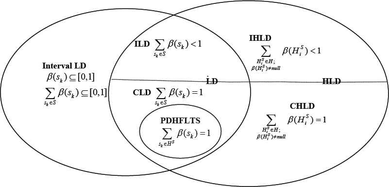
The relationships among LD and its variants
5. Use of the proposed HLDs in MAGDM
In this section, we apply our proposal in MAGDM problems [6, 8, 38, 40]. Procedures for MAGDM with HLDs are presented and an illustrative example is demonstrated.
5.1. Description of the MAGDM problem with HLDs
In this section we propose the procedures for the MAGDM with HLDs.
Let S = {s0, s1,…, sg} be the linguistic term set and D = {d1, d2,…, dn} be a set of n decision makers with w = {w1, w2,…, wn}T being the weighting vector satisfying wj ≥ 0 and
Step 1: Construct the evaluation matrix of each decision maker dj (j = 1,2,…, n) for alternatives {x1, x2,…, xq},
The HLD based evaluation matrix
Step 2: Obtain the collective evaluation matrix
Without loss of generality, we utilize the HLDOWA in the aggregation process in this step and the next step. Then based on Eq. (8), we obtain
Step 3: Calculate the overall value zr of each alternative xr.
zr is computed by
Step 4: Rank the alternatives {x1, x2,…, xq}.
According to the comparisons for HLDs in section 3 and the Algorithm I, we rank the alternatives based on the expectations and variations of zr by Eqs. (4)–(5). The larger value of E(zr), the better alternative xr.
5.2. Illustrative example
Suppose that five experts, D = {d1, d2, d3, d4, d5}, are invited to provide professional evaluations on football teams. Four football teams, X = {x1, x2, x3, x4}, are considered and four attributes A = {a1, a2, a3, a4} are taken into account in the evaluation process. The information of the football teams provided for the experts are each team’s previous performances, so experts {d1, d2, d3, d4, d5} provide their preferences over {x1, x2, x3, x4} by the form of LDs. As the expert team consists of experts from different fields, who may hesitate when evaluating due to their vague knowledge for the football teams, the HLDs are adopted by experts to elicit their preferences. The established linguistic term set is
Step 1: Five experts’ evaluation matrices for alternative xr (r = 1,2,3,4) are listed below. See Tables 2–6.
Step 2: Obtain the collective evaluation
Step 3: Calculate the overall value zr of each alternative xr (r = 1,2,3,4) by Eq. (14). Without loss of generality, suppose v = (0.15,0.3,0.25,0.3)T. See Table 8.
Step 4: Rank the alternatives {x1, x2, x3, x4} according to the expectations of zr (r = 1,2,3,4). Based on the Algorithm I, we have the transformed LDs
| L1 | a1 | a2 | a3 | a4 |
|---|---|---|---|---|
| x1 | {(s0, 0.2), ({s1, s2}, 0.2), ({s3, s4}, 0.3), ({s5, s6}, 0.3)} |
{({s0, s1}, 0.1), ({s2, s3}, 0.2), (s3, 0.2), ({s4, s5, s6}, 0.5)} |
{({s0, s1}, 0.1), (s2, 0.1), ({s3, s4}, 0.2), ({s4, s5, s6}, 0.6)} |
{(s0, 0.2), ({s1, s2, s3}, 0.2), ({s4, s5, s6}, 0.6)} |
| x2 | {({s0, s1}, 0.1), ({s2, s3}, 0.2), ({s3, s4, s5}, 0.4), ({s5, s6}, 0.3)} |
{({s0, s1}, 0.2), ({s2, s3}, 0.2), ({s3, s4}, 0.3), ({s5, s6}, 0.3)} |
{(s0, 0.1), ({s1, s2, s3}, 0.4), ({s4, s5}, 0.3), ({s5, s6}, 0.2)} |
{({s0, s1, s2}, 0.4), (s3, 0.2), ({s4, s5, s6}, 0.4)} |
| x3 | {({s0, s1, s2}, 0.3), ({s3, s4}, 0.4), ({s5, s6}, 0.3)} |
{(s0, 0.1), ({s1, s2, s3}, 0.3), (s4, 0.3), ({s5, s6}, 0.3)} |
{({s0, s1, s2}, 0.4), ({s3, s4, s5}, 0.4), (s6, 0.2)} |
{({s0, s1}, 0.2), (s2, 0.1), ({s3, s4, s5, s6}, 0.7)} |
| x4 | {({s0, s1}, 0.1), ({s2, s3, s4}, 0.4), ({s3, s4}, 0.2), ({s4, s5}, 0.2), (s6, 0.1)} |
{({s0, s1, s2}, 0.2), (s3, 0.1), ({s3, s4}, 0.3), ({s5, s6}, 0.4)} |
{({s0, s1}, 0.3), ({s1, s2, s3}, 0.3), ({s4, s5, s6}, 0.4)} |
{(s0, 0.1), ({s0, s1, s2}, 0.4), ({s3, s4}, 0.2), ({s5, s6}, 0.3)} |
The linguistic preference L1 provided by d1.
| L2 | a1 | a2 | a3 | a4 |
|---|---|---|---|---|
| x1 | {(s0, s1, s2}, 0.4), ({s3, s4, s5}, 0.3), (s6, 0.3)} |
{({s0, s1}, 0.1), ({s2, s3, s4}, 0.4), ({s5, s6}, 0.5)} |
{({s0, s1}, 0.2), ({s2, s3, s4}, 0.3), ({s4, s5}, 0.2), ({s4, s5, s6}, 0.3)} |
{(s0, 0.1), (s1, 0.1) ({s2, s3}, 0.2), ({s4, s5, s6}, 0.6)} |
| x2 | {({s0, s1}, 0.1), ({s1, s2, s3}, 0.3), ({s3, s4}, 0.3), ({s5, s6}, 0.3)} |
{({s0, s1, s2, s3}, 0.5), ({s3, s4, s5, s6}, 0.5)} |
{(s0, 0.1), ({s1, s2, s3}, 0.4), ({s4, s5, s6}, 0.3), ({s5, s6}, 0.2)} |
{({s0, s1, s2}, 0.3), (s3, 0.2), (s4, 0.1), ({s4, s5, s6}, 0.4)} |
| x3 | (s1, 0.1), ({s2, s3, s4}, 0.4), ({s5, s6}, 0.3)} |
{(s0, 0.1), ({s1, s2}, 0.3), ({s3, s4}, 0.3), (s5, 0.2), (s6, 0.1)} |
{({s0, s1, s2}, 0.4), ({s3, s4,}, 0.3), (s5, 0.1), ({s5, s6}, 0.2)} |
{({s0, s1}, 0.2), (s2, 0.1), ({s3, s4, s5}, 0.6), ({s5, s6}, 0.1)} |
| x4 | {(s0, 0.1), ({s1, s2, s3}, 0.3), ({s3, s4}, 0.2), ({s4, s5}, 0.2), (s6, 0.2)} |
{({s0, s1}, 0.1), (s2, 0.1), (s3, 0.1), ({s3, s4}, 0.2), ({s4, s5, s6}, 0.5)} |
{({s0, s1}, 0.2), ({s1, s2, s3}, 0.3), ({s4, s5, s6}, 0.3), ({s5, s6}, 0.2)} |
{(s0, 0.1), ({s0, s1, s2}, 0.4), ({s2, s3, s4}, 0.3), ({s5, s6}, 0.2)} |
The linguistic preference L2 provided by d2.
| L3 | a1 | a2 | a3 | a4 |
|---|---|---|---|---|
| x1 | {(s0, 0.1), (s1, 0.1), (s2, 0.1), ({s3, s4, s5}, 0.3), ({s5, s6}, 0.4)} |
{({s0, s1}, 0.1), (s1, 0.1), (s2, 0.1) (s3, 0.2), ({s2, s3, s4}, 0.3), ({s5, s6}, 0.2)} |
{({s0, s1}, 0.2), ({s1, s2, s3}, 0.3), (s4, 0.2), (s5, 0.1), (s6, 0.2)} |
{(s0, 0.1), (s1, 0.1) ({s0, s1, s2}, 0.2), (s3, 0.1), ({s4, s5, s6}, 0.5)} |
| x2 | {({s0, s1, s2}, 0.2), ({s1, s2}, 0.2), ({s3, s4, s5}, 0.3), ({s5, s6}, 0.3)} |
{({s0, s1}, 0.1), ({s1, s2, s3}, 0.3) ({s3, s4, s5}, 0.4), ({s5, s6}, 0.2)} |
{(s0, 0.1), ({s0, s1}, 0.2), ({s1, s2, s3}, 0.3), ({s4, s5}, 0.3), ({s5, s6}, 0.1)} |
{({s0, s1, s2}, 0.3), (s2, 0.1), (s3, 0.2), (s4, 0.1), ({s4, s5, s6}, 0.3)} |
| x3 | {({s0, s1}, 0.2), ({s1, s2}, 0.1), ({s2, s3, s4}, 0.4), ({s4, s5, s6}, 0.3)} |
{(s0, 0.1), ({s1, s2}, 0.2), (s2, 0.1), ({s3, s4}, 0.3), ({s4, s5}, 0.2), (s6, 0.1)} |
{({s0, s1, s2}, 0.3), ({s3, s4}, 0.3), ({s4, s5}, 0.1), ({s5, s6}, 0.3)} |
{({s0, s1}, 0.2), (s2, 0.1), (s3, 0.1), ({s3, s4, s5}, 0.3), (s4, 0.1), ({s5, s6}, 0.2)} |
| x4 | {(s0, 0.1), ({s1, s2}, 0.2) ({s1, s2, s3}, 0.3), ({s3, s4, s5}, 0.3), ({s5, s6}, 0.1)} |
{({s0, s1}, 0.1), (s2, 0.1), (s3, 0.1), ({s2, s3, s4}, 0.3), ({s5, s6}, 0.4)} |
{({s0, s1}, 0.2), ({s1, s2}, 0.2), ({s3, s4, s5, s6}, 0.4), ({s5, s6}, 0.1), (s6, 0.1)} |
{(s0, 0.1), ({s0, s1}, 0.2), ({s0, s1, s2}, 0.3), ({s3, s4}, 0.2), ({s5, s6}, 0.2)} |
The linguistic preference L3 provided by d3.
| L4 | a1 | a2 | a3 | a4 |
|---|---|---|---|---|
| x1 | {(s0, 0.1), (s1, 0.1), (s2, 0.1), (s3, 0.1), ({s4, s5, s6}, 0.6)} |
{({s0, s1}, 0.1), (s1, 0.1), (s2, 0.1) (s3, 0.2), (s4, 0.1), ({s5, s6}, 0.4)} |
{({s0, s1, s2}, 0.3), ({s2, s3}, 0.3), (s4, 0.1), (s5, 0.2), (s6, 0.1)} |
{({s0, s1, s2}, 0.3), (s3, 0.1), ({s4, s5, s6}, 0.6)} |
| x2 | {({s0, s1, s2}, 0.3), (s3, 0.2), (s4, 0.2), (s5, 0.1), (s6, 0.2)} |
{({s0, s1, s2}, 0.3), ({s3, s4}, 0.2), (s5, 0.3), (s6, 0.2)} |
{({s0, s1}, 0.2), ({s1, s2, s3}, 0.3), (s4, 0.1), (s5, 0.2), (s6, 0.2)} |
{(s0, 0.1), ({s0, s1, s2}, 0.3), (s2, 0.1), (s3, 0.2), (s4, 0.1), ({s5, s6}, 0.2)} |
| x3 | {({s0, s1}, 0.2), (s2, 0.1), ({s2, s3}, 0.3), (s4, 0.1), ({s5, s6}, 0.3)} |
{({s0, s1}, 0.2), ({s2, s3}, 0.3), (s3, 0.1), (s4, 0.1), (s5, 0.1), ({s5, s6}, 0.2)} |
{({s0, s1}, 0.2), ({s2, s3, s4}, 0.3), (s5, 0.2), ({s5, s6}, 0.2), (s6, 0.1)} |
{(s0, 0.1), ({s1, s2}, 0.2), ({s3, s4, s5}, 0.3), {(s4, s5, s6}, 0.3), (s6, 0.1)} |
| x4 | {(s0, 0.1), ({s1, s2}, 0.2) (s3, 0.3), (s4, 0.1), (s5, 0.2), (s6, 0.1)} |
{(s0, 0.1), ({s1, s2, s3}, 0.3), (s4, 0.2), (s5, 0.2), (s6, 0.2)} |
{(s0, 0.1), ({s1, s2, s3, s4}, 0.6), (s5, 0.2), (s6, 0.1)} |
{({s0, s1}, 0.2), ({s2, s3, s4, s5}, 0.5), (s6, 0.3)} |
The linguistic preference L4 provided by d4.
| L5 | a1 | a2 | a3 | a4 |
|---|---|---|---|---|
| x1 | {(s0, 0.1), (s1, 0.1) (s2, 0.1), ({s3, s4}, 0.1), ({s4, s5, s6}, 0.6)} |
{(s0, 0.1), (s1, 0.1), (s2, 0.1), (s3, 0.2), (s4, 0.2), ({s5, s6}, 0.3)} |
{({s0, s1}, 0.2), (s1, 0.1), (s2, 0.1) (s3, 0.1), (s4, 0.1), (s5, 0.1), ({s5, s6}, 0.3)} |
{(s0, 0.1), (s1, 0.1), (s2, 0.1), (s3, 0.2), (s4, 0.2), (s5, 0.1), ({s5, s6}, 0.2)} |
| x2 | {({s0, s1, s2}, 0.3), (s2, 0.1), (s3, 0.2), (s4, 0.1), (s5, 0.1), (s6, 0.2)} |
{(s0, 0.1),{s1, s2, s3}, 0.3), (s3, 0.1), (s4, 0.1), (s5, 0.2), (s6, 0.2)} |
{(s0, 0.1), (s1, 0.2), ({s2, s3, s4}, 0.3), (s4, 0.1), (s5, 0.1), (s6, 0.2)} |
{(s0, 0.1), (s1, 0.2), (s2, 0.1),{s3, s4, s5}, 0.3), (s6, 0.3)} |
| x3 | {({s0, s1}, 0.2), (s2, 0.1), (s3, 0.3), (s4, 0.1), ({s5, s6}, 0.3)} |
{({s0, s1}, 0.2), ({s2, s3}, 0.3), (s4, 0.1), (s5, 0.1), ({s4, s5, s6}, 0.3)} |
{(s0, 0.2),{s1, s2}, 0.2), ({s3, s4}, 0.3), (s5, 0.1), (s6, 0.2)} |
{(s0, 0.1), ({s1, s2, s3}, 0.3), ({s3, s4, s5}, 0.3), {(s4, s5, s6}, 0.3)} |
| x4 | {(s0, 0.1), (s1, 0.1), (s2, 0.2) (s3, 0.1), (s4, 0.2), (s5, 0.2), (s6, 0.1)} |
{(s0, 0.2), ({s1, s2, s3}, 0.3), ({s4, s5}, 0.2), ({s4, s5, s6}, 0.3)} |
{(s0, 0.2), ({s1, s2, s3, s4, s5}, 0.6), (s6, 0.2)} |
{({s0, s1}, 0.2), (s2, s3, s4, s5, s6}, 0.8)} |
The linguistic preference L5 provided by d5.
| a1 | a2 | a3 | a4 | |
|---|---|---|---|---|
| x1 | {(s0, 0.1), ({s0, s1, s2}, 0.08), (s1, 0.06), ({s1, s2}, 0.04), (s2, 0.06), (s3, 0.02), ({s3, s4}, 0.08), ({s3, s4, s5}, 0.12), ({s4, s5, s6}, 0.24), ({s5, s6}, 0.14), (s6, 0.06)} |
{(s0, 0.02), ({s0, s1}, 0.08), (s1, 0.06), (s2, 0.06), ({s2, s3}, 0.04), ({s2, s3, s4}, 0.14), (s3, 0.16), (s4, 0.06), ({s4, s5, s6}, 0.1), ({s5, s6}, 0.28)} |
{({s0, s1}, 0.14), ({s0, s1, s2}, 0.06), (s1, 0.02), ({s1, s2, s3}, 0.06), (s2, 0.04), ({s2, s3}, 0.06), ({s2, s3, s4}, 0.06), (s3, 0.02), ({s3, s4}, 0.04), (s4, 0.08), ({s4, s5}, 0.04), ({s4, s5, s6}, 0.18), (s5, 0.08), ({s5, s6}, 0.06), (s6, 0.06)} |
{(s0, 0.1), ({s0, s1, s2}, 0.1), (s1, 0.06), ({s1, s2, s3}, 0.04), (s2, 0.02), ({s2, s3}, 0.04), (s3, 0.08), (s4, 0.04), ({s4, s5, s6}, 0.46), (s5, 0.02), ({s5, s6}, 0.04)} |
| x2 | {({s0, s1}, 0.04), ({s0, s1, s2}, 0.16), ({s1, s2}, 0.04), ({s1, s2, s3}, 0.06), (s2, 0.02), ({s2, s3}, 0.04), (s3, 0.08), ({s3, s4}, 0.06), ({s3, s4, s5}, 0.14), (s4, 0.06), (s5, 0.04), ({s5, s6}, 0.18), (s6, 0.08)} |
{(s0, 0.02), ({s0, s1}, 0.06), ({s0, s1, s2}, 0.06), ({s0, s1, s2, s3}, 0.1), ({s1, s2, s3}, 0.12), ({s2, s3}, 0.04), (s3, 0.02), ({s3, s4}, 0.1), ({s3, s4, s5}, 0.08), ({s3, s4, s5, s6}, 0.1), (s4, 0.02), (s5, 0.1), ({s5, s6}, 0.1), (s6, 0.08)} |
{(s0, 0.12), ({s0, s1}, 0.04), (s1, 0.04), ({s1, s2, s3}, 0.28), ({s2, s3, s4}, 0.06), (s4, 0.04), ({s4, s5}, 0.12), ({s4, s5, s6}, 0.06), (s5, 0.06), ({s5, s6}, 0.1), (s6, 0.08)} |
{(s0, 0.04), ({s0, s1, s2}, 0.26), (s1, 0.04), (s2, 0.06), (s3, 0.16), ({s3, s4, s5}, 0.06), (s4, 0.06), ({s4, s5, s6}, 0.22), ({s5, s6}, 0.04), (s6, 0.06)} |
| x3 | {({s0, s1}, 0.16), ({s0, s1, s2}, 0.06), (s1, 0.02), ({s1, s2}, 0.02), (s2, 0.04), ({s2, s3}, 0.06), ({s2, s3, s4}, 0.16), (s3, 0.06), ({s3, s4}, 0.08), (s4, 0.04), ({s4, s5, s6}, 0.06), ({s5, s6}, 0.24)} |
{(s0, 0.06), ({s0, s1}, 0.08), ({s1, s2}, 0.1), ({s1, s2, s3}, 0.06), (s2, 0.02), ({s2, s3}, 0.12), (s3, 0.02), ({s3, s4}, 0.12), (s4, 0.1), ({s4, s5}, 0.04), ({s4, s5, s6}, 0.06), (s5, 0.08), ({s5, s6}, 0.1), (s6, 0.04)} |
{(s0, 0.04), ({s0, s1}, 0.04), ({s0, s1, s2}, 0.22), ({s1, s2}, 0.04), ({s2, s3, s4}, 0.06), ({s3, s4}, 0.18), ({s3, s4, s5}, 0.08), ({s4, s5}, 0.02), (s5, 0.08), ({s5, s6}, 0.14), (s6, 0.1)} |
{(s0, 0.04), ({s0, s1}, 0.12), ({s1, s2}, 0.04), ({s1, s2, s3}, 0.06), (s2, 0.06), (s3, 0.02), ({s3, s4, s5}, 0.3), ({s3, s4, s5, s6}, 0.14), (s4, 0.02), ({s4, s5, s6}, 0.12), ({s5, s6}, 0.06), (s6, 0.02)} |
| x4 | {(s0, 0.08), ({s0, s1}, 0.02), (s1, 0.02), ({s1, s2}, 0.08), ({s1, s2, s3}, 0.12), (s2, 0.04), ({s2, s3, s4}, 0.08), (s3, 0.08), ({s3, s4}, 0.08), ({s3, s4, s5}, 0.06), (s4, 0.06), ({s4, s5}, 0.08), (s5, 0.08), ({s5, s6}, 0.02), (s6, 0.1)} |
{(s0, 0.06), ({s0, s1}, 0.04), ({s0, s1, s2}, 0.04), ({s1, s2, s3}, 0.12), (s2, 0.04), ({s2, s3, s4}, 0.06), (s3, 0.06), ({s3, s4}, 0.1), (s4, 0.04), ({s4, s5}, 0.04), (s5, 0.04), ({s4, s5, s6}, 0.16), ({s5, s6}, 0.16), (s6, 0.04)} |
{(s0, 0.06), ({s0, s1}, 0.14), ({s1, s2}, 0.04), ({s1, s2, s3}, 0.12), ({s1, s2, s3, s4}, 0.12), ({s1, s2, s3, s4, s5}, 0.12), ({s3, s4, s5, s6}, 0.08), ({s4, s5, s6}, 0.14), (s5, 0.04), ({s5, s6}, 0.06), (s6, 0.08)} |
{(s0, 0.06), ({s0, s1}, 0.12), ({s0, s1, s2}, 0.22), ({s2, s3, s4}, 0.06), ({s2, s3, s4, s5}, 0.1), ({s2, s3, s4, s5, s6}, 0.16), ({s3, s4}, 0.08), ({s5, s6}, 0.14), (s6, 0.06)} |
The collective linguistic preference
| zr (r = 1,2,3,4) | |
|---|---|
| x1 | {(s0, 0.058), ({s0, s1, s2}, 0.067), ({s0, s1}, 0.054), (s1, 0.048), ({s1, s2}, 0.012), ({s1, s2, s3}, 0.028), (s2, 0.044), ({s2, s3}, 0.034), ({s2, s3, s4}, 0.039), (s3, 0.056), ({s3, s4}, 0.036), ({s3, s4, s5}, 0.036), (s4, 0.043), ({s4, s5}, 0.012), ({s4, s5, s6}, 0.256), (s5, 0.029), ({s5, s6}, 0.112), (s6, 0.036)} |
| x2 | {(s0, 0.045), ({s0, s1}, 0.031), ({s0, s1, s2}, 0.135), ({s0, s1, s2, s3}, 0.015), (s1, 0.022), ({s1, s2}, 0.012), ({s1, s2, s3}, 0.106), (s2, 0.024), ({s2, s3}, 0.018), ({s2, s3, s4}, 0.015), (s3, 0.075), ({s3, s4}, 0.033), ({s3, s4, s5}, 0.072), ({s3, s4, s5, s6}, 0.015), (s4, 0.049), ({s4, s5}, 0.03), ({s4, s5, s6}, 0.081), (s5, 0.042), ({s5, s6}, 0.106), (s6, 0.074)} |
| x3 | {{(s0, 0.033), ({s0, s1}, 0.098), ({s0, s1, s2}, 0.084), (s1, 0.006), ({s1, s2}, 0.049), ({s1, s2, s3}, 0.024), (s2, 0.026), ({s2, s3}, 0.048), ({s2, s3, s4}, 0.066), (s3, 0.026), ({s3, s4}, 0.108), ({s3, s4, s5}, 0.069), ({s3, s4, s5, s6}, 0.021), (s4, 0.04), ({s4, s5}, 0.016), ({s4, s5, s6}, 0.051), (s5, 0.044), ({s5, s6}, 0.148), (s6, 0.043)} |
| x4 | {{(s0, 0.066), ({s0, s1}, 0.083), ({s0, s1, s2}, 0.072), (s1, 0.006), ({s1, s2}, 0.034), ({s1, s2, s3}, 0.084), ({s1, s2, s3, s4}, 0.03), ({s1, s2, s3, s4, s5}, 0.03), (s2, 0.018), ({s2, s3, s4}, 0.051), ({s2, s3, s4, s5}, 0.03), ({s2, s3, s4, s5, s6}, 0.048), (s3, 0.033), ({s3, s4}, 0.063), ({s3, s4, s5}, 0.018), ({s3, s4, s5, s6}, 0.02), (s4, 0.024), ({s4, s5}, 0.03), ({s4, s5, s6}, 0.059), (s5, 0.04), ({s5, s6}, 0.087), (s6, 0.074)} |
The overall value of alternative xr (r 1,2,3,4).
| x1 | {(s0, 0.1073), (s1, 0.1127), (s2, 0.1117), (s3, 0.1253),, (s4, 0.1773), (s5, 0.1883), (s6, 0.1773)} |
| x2 | {{(s0, 0.10925), (s1, 0.1276), (s2, 0.1281), (s3, 0.1723), (s4, 0.14025), (s5, 0.16475), (s6, 0.15775)} |
| x3 | {{(s0, 0.11), (s1, 0.1155), (s2, 0.1325), (s3, 0.16225), (s4, 0.16925), (s5, 0.17125), (s6, 0.13925)} |
| x4 | {(s0, 0.1315), (s1, 0.13), (s2, 0.1346), (s3, 0.1511),, (s4, 0.1488), (s5, 0.1523), (s6, 0.1517)} |
The transformed LDs
As E(z1) > E(z3) > E(z2) > E(z4), the ranking of the alternatives is: x1 ≻ x3 ≻ x2 ≻ x4.
6. Conclusions
In this paper, we propose the concept of the HLD to model decision makers’ linguistic expression preferences based on the use of HFLTSs and LDs, and study the proposed HLD from the following aspects.
- (1)
The transformation between the HLDs and LDs is presented and basic operations including comparison and aggregation operations are proposed to perform on HLDs.
- (2)
The comparisons among several linguistic expressions such as the PDHFLTS, CLD, ILD, and interval LD and HLD are discussed to show that the HLD is their generalization.
- (3)
We discuss the use and behavior mechanism of the HLD in MAGDM.
The GDM with linguistic expressions not only relates to mathematical models, but also to philosophical issues. Therefore, it would be interesting to psychologically investigate decision makers’ behaviors when using different linguistic expressions in the future research.
Acknowledgements
This work was supported by the grants (Nos. 71201122, 71571124) from NSF of China.
References
Cite this article
TY  - JOUR
AU  - Guiqing Zhang
AU  - Yuzhu Wu
AU  - Yucheng Dong
PY  - 2017
DA  - 2017/06/28
TI  - Generalizing linguistic distributions in hesitant decision context
JO  - International Journal of Computational Intelligence Systems
SP  - 970
EP  - 985
VL  - 10
IS  - 1
SN  - 1875-6883
UR  - https://doi.org/10.2991/ijcis.2017.10.1.65
DO  - 10.2991/ijcis.2017.10.1.65
ID  - Zhang2017
ER  -