
Multi-stage method to identify structural damage using multiple damage location assurance criterion and an improved differential evolution algorithm
- DOI
- 10.2991/ijcis.2017.10.1.71How to use a DOI?
- Keywords
- damage identification; multiple damage location assurance criterion; improved differential evolution algorithm; multi-stage method; adaptive scaling factor
- Abstract
For the damage identification technique of civil structures, the reduction of the computational cost for methods based on the optimization algorithms is the most crucial step. In this study, a fast multi-stage method is developed that uses the multiple damage location assurance criterion and an improved differential evolution algorithm. In the new method, the suitable damage range is selected in different stages to reduce the computational cost of structural analysis. Five mutation operators are analysized not only in the basic differential evolution algorithm but also in the improved one. A new adaptive scaling factor with a segmented function is proposed which can operate the decay rate to avoid the premature phenomenon. The results of the study show that the precise locations and extents of structural damage are successfully realized. It is also shown that the multi-stage method using the improved differential evolution algorithm is substantially faster as compared to the basic one and can be used as an efficient and powerful measure of structural damage identification.
- Copyright
- © 2017, the Authors. Published by Atlantis Press.
- Open Access
- This is an open access article under the CC BY-NC license (http://creativecommons.org/licences/by-nc/4.0/).
1. Introduction
Civil engineering structures have always been susceptible to various kinds of damage during their service life due to environmental, operational and human-induced factors. Therefore, damage identification has been essential issues for determining safety reliability and remaining lifetime of structures. Although a mass of damage identification methods are proposed in the many literatures in the past several decades, the vibration-based structural damage detection has been one of the best hot issues of research. The basic idea of the vibration-based damage identification approaches is that the changes in the physical properties (mass, stiffness and daming) due to damage will be reflected in modal proprerties (frequencies, mode shapes and modal damping). Hence, the damage identification as an inverse problem can be realized by detecting the changes of modal properties before and after damage by using the finite element model and given limited modal data measured from a real structure. Reviews of these methods can be found in Refs. 1–5. More study efforts had been implemented based on frequency change-based method 6, 7, mode shape change-based method 8–10, frequency and mode shape change-based method11, mode shape curvature 12,13, modal strain enery 14,15, flexibility based approach 16, 17, and frequency response function18–19.
Intelligence optimal algorithms have been widely employed for structural damage detection. The main idea of optimal algorithms is transforming the damage identification problem into an optimization problem in which the objective function composed by the alteration between the FEM and measured data is usually minimized or maxmized. So far, an increasing number of optimal algorithms such as neural network (NE) 20,21, Genetic algorithms (GA)22, 23, particle swarm optimization (PSO)24, 25, artificial bee colony (ABC)26, 27, differential evolution (DE)28–30 and wavelet analysis 31,32 etc are widely used in determining the location and extent of structural damage. However, the expensive computational cost and the invalid for dealing with large civil engineering structures of the optimization algorithms still need to be addressed eagerly.
Phased approaches such as two-step and multi-stage methods using in detecting both the damage location and extent have been employed to reduce the expensive computational cost. Two-stage method is the most common, in which the possible damage sites are determined in the first stage using certain modal indicators, for examples, the modal strain energy 28, evidence theory combined with natural frequencies and mode shapes22, modal residual vector 29, modal strain energy and frequency integrated with Bayesian theory 23, and the damage extents are detected in the next stage by the use of an improved DE 28, micro-search GA22, GA29, immune GA23 with respect to the examples of the first stage. Further more, the multi-stage methods are proposed in few researches. Grande33 proposed a multi-stage approach with the mode shapes assumed as primary sources and local decisions based on a flexibility method. Nevertheless, the high computational cost of detecting damage locations, especially the damage extents of the large structures still is an urgent task to resolve for damage identification technique based on optimal algorithms.
This paper makes an effort to further reduce the computational cost of detecting damage sites and extents of civil engineering structures by proposing a multi-stage method with multiple damage location assurance criterion (MDLAC) and an improved differential evolution (IDE) algorithm. Unlike the other researches, in this paper, MDLAC is regarded as the objective function of optimal algorithm and that differential evolution algorithm is as the optimal tool in each stage. For the present multi-stage method, the small damage range and filtering threshold are used in the earlier stage to reduce the design variables of the optimization problem for the later stages. Moreover, this paper analyzes and compares five mutation operators and different scaling factors, and proposes a new adaptive scaling factor with a segmented function in order to find the more efficient mutation operator. The numerical examples consider a continous beam and a square composite plate, as well as the effect of noise on the accuracy of the present procedure is investigated. The results of the study show that regardless of the effect of noise, the precise locations and extents of structural damage are successfully realized, especially for the computational cost.
This study is organized as follows: In Section 2, damage indexes based on the natural frequency, mode shape and both the frequency and mode shape are presented, respectively. Section 3 gives the introduction of the basic differential evolution algorithm and the improved differential evolution algorithm in terms of the scale factor F. In Sections 4, the multi-stage damage identification method is proposed including the individual, damage range and filtering threshold. In Sections 5, the performance of the multi-stage damage identification method is demonstrated with a continous beam and a square composite plate.
2. Damage indices of multiple damage locations
2.1. Damage index based on natural frequency
MDLAC is a powerful tool to identify the location and extent of damage existing in structures, which is performed by considering the correlation between the modal parameters monitored in practical structures and parameters calculated by Finite Element Analysis (FEA) 34–36.
The natural frequency is first used, and afterwards the mode shape is introduced in the MDLAC. When only the natural frequency is considered, MDLAC_f can be expressed as
The values of MDLAC_f vary between zero and one. A value of zero denotes no correlation between the measured and theoretical frequency shift, and a value of one indicates exact match, i.e. F(X) = Fd. This shows that the highest value of MDLAC_f is optimal for determining the location and extent of damage.
2.2. Damage index based on mode shape
The processes of damage detection using the MDLAC based on natural frequency are demonstrated commonly by the symmetrical structure, for example, a cantilever beam in Refs.34 and 35. However, only the MDLAC with respect to the frequency fails to asymmetric structures, especially such as civil engineering structures. As a consequence, the mode shape owing to the excellent local sensitivity for damage is introduced to the damage index of MDLAC. The MDLAC_Φ is given by
Similar to considering the frequency, the values of MDLAC_Φ vary between zero and one. A value of zero denotes no correlation and one indicates exact match, i.e. Φ(X) = Φd. Therefore, the aim of damage identification focuses on maximizing the value of MDLAC_Φ by finding the vector X contained the degree of damage.
2.3. Damage index based on both frequency and mode shape
A MDLAC_f + Φ is proposed based on both frequencies and mode shapes, which can address well both symmetrical and asymmetrical structures35, 36. This combined index is defined by
Now, the problem of damage identification can be solved by searching the vector X to maximize the index MDLAC_f + Φ. An optimization algorithm is required to solve this issue, and the optimization process can be described as follows.
3. Differential evolution algorithm
3.1. Basic differential evolution algorithm
Differential Evolution (DE) Algorithm is a global search algorithm inspired by Darwin’s survival-of-the-fittest theory, which can also obtain the optimal solution by three main operators including the mutation, cross and selection28–30. Provided that the individual of the Gth generation is Xi,G and i = 1,2,⋯, NP, in which NP is the population size, some basic concepts and operators of a DE can be introduced as follows.
3.1.1. Coding
An essential characteristic of a DE is the coding of the individuals that describe the optimization problem. The real coding can be written as Xi,G = (x1, x2,⋯, xD).
3.1.2. Initial population
The following expression is used to initialize population.
3.1.3. Mutation
The mutation operator is a main step to generate the new individuals in the DE. At the same time, this operator is the biggest difference between the DE and GA or other algorithms. The middle individuals after the process of the mutation are Yi,G, which can be obtained by the linear combinations as follows.
rand1:
rand2:
best1:
best2:
current to rand:
current to best:
It should be noted that F is an essential parameter in DE because it improves the diversity of population. A small F will lead to extensive exploitation in the search space, whereas a large F will lead to over exploration and low convergence speed.
3.1.4. Crossover
The crossover operator can further promote the diversity of population by hybridizing the individuals Yi,G and Xi,G. Assuming that the new candidate solutions are Ui,G, and it can be written as Ui,G = (u1i,G,u2i,G,⋯, uDi,G), in which i = 1,2,⋯, NP and j = 1,2,⋯, D. The new individual by the crossover operation uji,G can be expressed in the form:
3.1.5. Selection
The selection operator is executed by comparing the fitness function values between the individuals Ui,G and Xi,G. The process can be expressed as
It can be shown from Eq. (17) that the selection operator is after the mutation and crossover operators in the DE algorithm, which is different from the GA. It is better that the parent individuals competing with the new candidate individuals one by one generate the new individuals on the equal opportunity.
3.2. Improved differential evolution algorithm
Many researches denote that the value of the scale factor F should be large in the initial stage of the algorithm such that the algorithm can maintain the diversities of the individuals, search the global optimum value and speed up the convergence speed of the optimal solution so as to avoid the premature phenomenon. While in a later stage of the algorithm, the speed of the scale factor F should be decreased, which should make it easy to search for the local optimum value 37, 38. The dynamic adaptive adjustment equation for the scale factor F is shown as follows.
Moreover, in Ref. 39, the value of F is generated for each individual from a normal distribution F ∈ N(0.5, 0.3), while the value is determined as F ∈ N(0, 1) in Ref. 40.
In the present IDE, the segmented function is utilized as the adaptive scaling factor provided in Eq. (19).
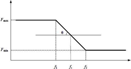
Scaling factor using segmented function
4. Multi-stage damage identification
In this paper, the IDE algorithms with different mutation strategies and different scaling factors are proposed to identify the damage sites and extents in the structures. Some important control parameters are required in the process of implementing the multi-stage damage identification, such as the individual, damage range and filtering threshold, which are introduced in the following.
4.1. Individual
The individual can be expressed as XT = {x1,x2,⋯, xi,⋯, xD}, in which xi represents the damage of the structures mentioned earlier. In most studies of damage detection, the damage is represented by the stiffness reduction because the damage of structural elements must lead to the stiffness descending. Hence, the damage is simulated by a reduction in the bending stiffness as
In this paper, we suppose the inertia moment I is constant and the damage is caused by the descending of elastic modulus E.
4.2. Damage range
In the present damage identification algorithm, damage range is a crucial parameter to quickly identify the damage location and extent using the present multi-stage method. The damage value R of the variable xi varies from zero to one. A value of zero means no damage and inversely a value of one denotes that the element in structures is totally damaged. A larger R will lead to a slow convergence speed and excessive iterations, while a smaller R will lead to leave out the optimal solutions (damaged elements). Therefore, R is a parameter which has a larger effect on the calculated amount and time of identifying the damage using the DE. In this paper, we suppose that the range of R value is less than and equal to 0.6 (the extent of damage is 60%). In fact, it is more reasonable because the occurrence of too much damage is a small probability event in actual structures. However, the calculated amount of the procedure is still considerably large even though R ∈ [0,0.6] due to the complicated structural analysis. Moreover, more elements divided in the model further increase the iterations from the other hand. In view of this, a multi-stage method is proposed to reduce the calculated amount and time of the search by controlling the range of R. For example, in Fig. 2, the first stage is to determine the range of R = [0,0.1] and then R = [0,0.6] in the second stage. In this way, in the first step, the running time is reduced due to the small damage range even though all elements involved in calculation. Consequently, a great amount of undamaged elements are filtering out and the locations of suspected damage elements are retained. Thus, a low calculated amount occurs because only the retained elements take part in the computation process of the second step even if the damage range is enlarged.
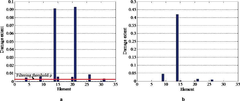
An example of the multi-step method to identify structural damage. (a) the first stage; (b) the second stage.
4.3. Filtering threshold
The filtering threshold ρ is a critical value to filter the undamaged elements and then retain the suspected damaged elements. A small ρ will lead to extensive suspected damaged elements retained and thus lose the multi-stage meaning, whereas a large ρ will lead to miss the damage elements. Fig. 2 shows an example of the two-step method to identify structural damage using the frequency MDLAC_f. In this example, damage occurs in elements 9 and 14 with 5% and 40% stiffness reduction, respectively. When the filtering threshold is selected as ρ = 0.0027 shown in Fig. 2 (a), only eight elements (4, 9, 14, 15, 20, 21, 26 and 31) are left as the suspected elements. Thereby, the relatively accurate damage results are quickly detected as the damages of element 9 with 4.98% and element 14 with 42% without the need for further filtering stage (Fig. 2 (b)).
The filtering threshold ρ can be expressed with the subscript ρ1 and ρ2 in the different stages of damage identification which can be defined by computing the average value of damage individuals as
4.4. Multi-stage damage identification
The damage location and extent of the structure are detected by the presented damage identification method. The flow chart of multi-stage method with MDLAC and DE or IDE is shown in Fig. 3.
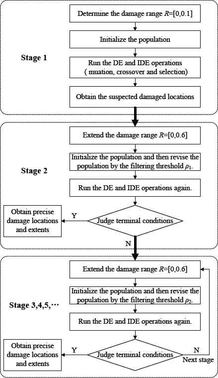
Flow chart of presented damage identification method.
5. Numerical studies
In this section, we present a numerical example of the continuous beam to verify the reliability of the proposed damage identification technique using the MDLAC and the IDE algorithm. Some control parameters in the DE and IDE are shown in Table 1.
| Parameter | Basic method | Multi-stage method (Present) | |
|---|---|---|---|
| DE | DE | IDE | |
| Size of population (NP) | 20 | 20 | 20 |
| Mutaion operator | rand1;rand2;best1;best2;current to rand | rand1;rand2;best1;best2;current to rand | rand1;rand2;best1;best2;current to rand |
| Scaling factor of mutation (F) | 0.8 | 0.8 | Exponential function, Segmented function |
| Crossover rate (CR) | 0.5 | 0.5 | 0.5 |
| Stop criterion | single criterion: objective function f | double criteria: Maximum iteration T and objective function f | double criteria: Maximum iteration T and objective function f |
Parameters of the DE and IDE using the multi-stage method
5.1. A continuous beam
5.1.1. Model of damage
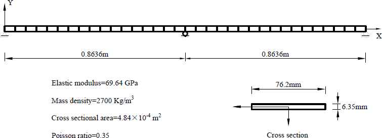
The first numerical example considered is a continuous beam with two spans shown in Fig. 4. The values of material and geometric properties for the beam are also given in the figure. The beam is divided into 34 equal length elements. The beam is excited by random dynamic loading which is stochastic in nature. A local damage is assumed by reducing the stiffness of element 9 by 5% and element 14 by 40%.
Schematic of continuous beam model.
5.1.2. Damage identification
In the whole process of damage identification, the damage index MDLAC with frequency and mode shape for all elements of the beam is computed by modal analysis of the FEM. Two cases without noise and with noise 3% and five muation strategies are considered respectively to verify the performance of damage identification. Both in the cases of noise-free and noise, the first ten frequencies and the fist three mode shapes are used to compute the objective damage index MDLAC. The individual can be denoted by XT = {x1,x2,⋯, xi,⋯, xD} (i = 1,⋯, D), which are the damage extents of D suspected elements. Particularly, for this example, XT = {x1,x2} in which x1 and x2 are the damage extents of the 9th and 14th elements, respectively. It should be noted that the statistical results are the average solutions of ten times precedure and the average number of structural analysis (NSA).
1. Case of noise free
In the case of noise free, the damage location and extent of damage elements are implemented by the comparison with the basic DE and the present multi-stage DE and IDE. The statistical results for five kinds of mutation strategies (rand1, rand2, best1, best2, current to rand (c t r)) are shown in Fig. 5 and Table 2. In these figures, the X, Y and Z axes are the number of elements, five kinds of mutation strategies and damage extent (1-MDLAC), respectively. In the basic DE, the single stop criterion is defined by the objective function f = 0.99998. While in the present DE and IDE, the double criteria in the different stages are set as the maximum iterations T1 = 5000, T2,3,⋯ = 1000, and objective functions f1 = 0.995, f2,3,⋯ = 0.99998, respectively. In addition, in the IDE, the proposed segmented function is used to improve the scaling factor F in the Stage 1, and the normal distribution F ∈ N(0.5, 0.3) is utilized in the subsequent stages. For the scaling factor of segmented function, some controlled parameters in Eq. (19) are set as: Fmax = 0.9, Fmin = 0.5, fs = 0.8, and θ = 80°.
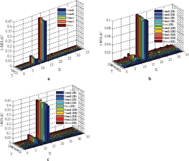
Results of damage identification using multi-stage method for DE and IDE. (a) basic DE; (b) Stage 1 of present DE and IDE, (c) Stage 2 of present DE and IDE.
| Mutation strategy | Basic DE | DE (present) | IDE (present) | |||||||||
|---|---|---|---|---|---|---|---|---|---|---|---|---|
| NSA | f | x1 | x2 | NSA | f | x1 | x2 | NSA | f | x1 | x2 | |
| rand1 | 9303 | 0.999980 | 0.052 | 0.408 | 4013 | 0.999997 | 0.049 | 0.398 | 2775 | 0.999995 | 0.050 | 0.394 |
| rand2 | 11875 | 0.999981 | 0.051 | 0.403 | 4630 | 0.999995 | 0.050 | 0.407 | 2981 | 0.999982 | 0.054 | 0.420 |
| best1 | 5797 | 0.999988 | 0.051 | 0.405 | 1284 | 0.999990 | 0.050 | 0.408 | 1170 | 0.999992 | 0.052 | 0.401 |
| best2 | 8544 | 0.999649 | 0.059 | 0.417 | 2597 | 0.999992 | 0.053 | 0.414 | 1353 | 0.999982 | 0.050 | 0.391 |
| c t r | 6296 | 0.999600 | 0.057 | 0.410 | 2717 | 0.999995 | 0.050 | 0.406 | 2908 | 0.999985 | 0.047 | 0.397 |
where, NSA=average number of structural analysis; f=the value of objective function x1=damage extent of element 9; x2=damage extent of element 14.
Statistical results of damage identification with basic DE and present DE and IDE
It can be seen that for the case of noise free from Fig. 5 and Table 2, the precise locations and extents of damaged elements can be detected by both the basic DE and the present DE and IDE under the computation of two stages. However, for the computaional cost, the NSA of the basic DE is more than the present multi_stage DE and IDE, while the IDE shows the preferable performance than the present DE due the less NSA. For different muataion strategies, the rand1 and rand2 are stable relatively, and that the best1 and best2 emerge the strong ability of computation, especially for the best1 with the least NSA.
2. Case of noise level 3%
In the case of measurement noise, the basic DE and the present mult-stage DE and IDE are used to detect the damage locations and extents. The statistical results for five kinds of mutation strategies are shown in Fig. 6 and Table 3. In these figures, the X, Y and Z axes are the number of elements, two kinds of mutation strategies and damage extent (1-MDLAC), respectively. In addition, the stop criteria in the multistage process need to be provided. They are: the maximum iterations T1 = 2000, T2,3,⋯ = 1000, and objective functions f1 = 0.9048, f2,3,⋯ = 0.92, respectively. It should be noted that the scaling facors and the relevent parameters used in this case are same with the case of noise free in different stages of the proposed multi-stage method.
| Mutation strategy | Basic DE | DE (present) | IDE (present) | |||||||||
|---|---|---|---|---|---|---|---|---|---|---|---|---|
| NSA | f | x1 | x2 | NSA | f | x1 | x2 | NSA | f | x1 | x2 | |
| rand1 | 11219 | 0.9228 | 0.084 | 0.347 | 4164 | 0.9243 | 0.062 | 0.387 | 4838 | 0.9288 | 0.051 | 0.388 |
| rand2 | 13527 | 0.9215 | 0.080 | 0.354 | 6879 | 0.9234 | 0.058 | 0.363 | 4847 | 0.9261 | 0.045 | 0.363 |
| best1 | 9479 | 0.9127 | 0.063 | 0.369 | 3266 | 0.9315 | 0.058 | 0.360 | 2944 | 0.9306 | 0.048 | 0.373 |
| best2 | 10636 | 0.9221 | 0.057 | 0.337 | 2801 | 0.9316 | 0.058 | 0.360 | 2321 | 0.9311 | 0.055 | 0.391 |
| c t r | 14190 | 0.9184 | 0.059 | 0.378 | 8879 | 0.9302 | 0.054 | 0.377 | 6134 | 0.9205 | 0.044 | 0.365 |
where, NSA=average number of structural analysis; f =the value of objective function x1=damage extent of element 9; x2=damage extent of element 14.
Statistical results of damage identification with basic DE and present DE and IDE
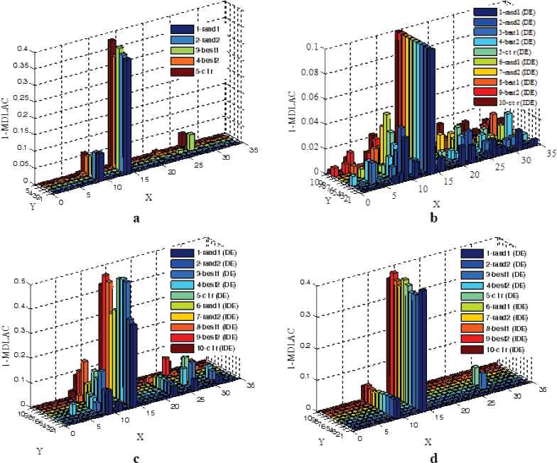
Results of damage identification using basic DE and present DE and IDE. (a) basic DE; (b) Stage 1 of present DE and IDE, (c) Stage 2 of present DE and IDE; Stage 3 of present DE and IDE.
It can be seen from Figs. 6 (a) and (d), and Table 3, the relatively accurate locations and extents of damaged elements can be detected by both the basic DE and the present DE and IDE with three computational stages. However, for the computational accuracy, the present the DE and IDE is better than the basic DE, especially for the IDE with the more optimal solutions. For the computational cost, the NSA of the basic DE is more than the present DE and IDE, while the IDE with the five mutation strategies except the rand1 show the preferable performance than the present DE due the less NSA. Especially, it is worth mentioning that the best1 and best2 are preferable due to the less NSA.
5.2. A square composite plate
5.2.1. Model of damage
The processes of multi-stage damage detection are also demonstrated using the laminated composite plate which is a three cross-ply (0 ° /90 ° /0 ° ) clamped composite plate shown in Fig. 7. The parameters of material are as follows:
- •
Length of a side a=1m,
- •
The thickness t=0.1m,
- •
Young’s Modulus E1=40N/m2,
- •
Young’s Modulus E2=1N/m2,
- •
Poisson ratio v12=0.25,
- •
Poisson ratio v21=0.00625.

(a) A square composite plate discretized by the FEM; (b) element numbering of the composite plate.
The free vibration behaviour of the composite plate was analysed in many literatures such as Ferreira et al. 41 using a first-order shear deformation theory and T. Vo-Duy et al. 28 using a two-step approach based on modal strain energy method and an improved differential evolution algorithm to detect the damage location and extent. In this example, the free vibration behaviour of the plate is obtained by the finte element method (FEM) using the ANSYS10.0, in which the plate is meshed 10 × 10 of 8-node shell99 element. Same as T. Vo-Duy et al. 28, the two damage scenarios consisting of two and three damaged elements are considered in Table 4. The first eight frquencies of the plate in the healthy and damaged stage are presented in Table 5.
| Scenario 1 | Scenario 2 | ||
|---|---|---|---|
| Element No. | Damage extent | Element No. | Damage extent |
| 37 | 0.4 | 33 | 0.15 |
| 47 | 0.6 | 57 | 0.2 |
| 74 | 0.25 | ||
Damage scenarios in the square composite plate
| Mode | Intact Ref. 28 | Damaged case 1 Ref. 28 | Damaged case 2 Ref. 28 | Intact (Present) | Damaged case 1 (Present) | Damaged case 2 (Present) |
|---|---|---|---|---|---|---|
| 1 | 7.444 | 7.377 | 7.422 | 7.415 | 7.393 | 7.410 |
| 2 | 10.438 | 10.377 | 10.400 | 10.456 | 10.435 | 10.442 |
| 3 | 13.990 | 13.850 | 13.951 | 13.947 | 13.888 | 13.928 |
| 4 | 15.520 | 15.378 | 15.458 | 15.621 | 15.576 | 15.596 |
| 5 | 15.887 | 15.813 | 15.841 | 15.926 | 15.902 | 15.906 |
| 6 | 19.686 | 19.552 | 19.622 | 19.824 | 19.785 | 19.803 |
| 7 | 21.627 | 21.022 | 21.482 | 21.556 | 21.541 | 21.550 |
| 8 | 21.813 | 21.602 | 21.726 | 22.044 | 21.983 | 22.025 |
First eight frequencies of the healthy and damaged stage in the square composite plate
5.2.2. Damage identification using the multi-stage method
For both scenarios of damage, the MDLAC is computed by using the first ten frequencies and the first two mode shapes for the case of noise-free and the first ten frquencies and the first two, four, five and six mode shapes for the case of considering the measurement noise. It should be noted that the statistical results are the average solutions of ten times precedure and the average number of structural analysis (NSA). Besides, the stop criteria and the scaling factors are same with the section 5.1 both in cases of noise-free and noise 3%.
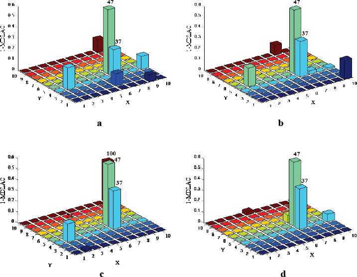
1. Case of noise free
In the case of noise free, only the present methods of the mult-stage DE and IDE are used to detect the damage locations and extents. The statistical result of mutation strategie (best1) is shown in Fig. 8 and Table 6.

Results of damage identification using the present DE and IDE without noise. (a) present DE of scenario 1; (b) present IDE of scenario 1; (c) present DE of scenario 2; (d) present IDE of scenario 2.
| Mutation strategy | Scenario 1 | Scenario 2 | |||||||
|---|---|---|---|---|---|---|---|---|---|
| NSA | f | x1 | x2 | NSA | f | x1 | x2 | x3 | |
| DE [28] | 7548 | 1.8519×10-08 | 0.400 | 0.600 | 8872 | 6.3076×10-07 | 0.150 | 0.200 | 0.250 |
| IDE [28] | 2660 | 4.3163×10-07 | 0.400 | 0.600 | 2520 | 4.5083×10-07 | 0.150 | 0.200 | 0.250 |
| DE (present) | 4174 | 0.999989 | 0.403 | 0.600 | 4788 | 0.999982 | 0.151 | 0.202 | 0.251 |
| IDE (present) | 3422 | 0.999982 | 0.398 | 0.599 | 3425 | 0.999993 | 0.151 | 0.201 | 0.252 |
where, NSA=average number of structural analysis; NS= number of stages; f =the value of objective function; for scenario 1: x1=damage extent of element 37, x2=damage extent of element 47; for scenario 2: x1=damage extent of element 33, x2=damage extent of element 57 and x3=damage extent of element 74.
Statistical results of damage identification for the square composite plate in the case of noise-free
Fig. 8 inllustrates that three damaged elements are located and quantitated exactly for the case of noise free without any false alarm elements by using the present DE and IDE. Table 6 indicates that the locations and extents of damaged elements are in good agreement with the corresponding results obtained by Ref. 28. However, it should be noted that the results of the NSA from Ref. 28 only include the quantification of damage severities without considering the computation amount of detecting the damage sites. It can be seen that the present IDE method with the new adaptive scaling factor is faster as compared to the present DE and the DE in Ref. 28, and that it isn’t too slow than the IDE in Ref. 28 although it counts the all stages of determining the damage sites and extents relative to Ref. 28.
2. Case of noise level 3%
Figs. 9 and 10 provide the statistical results in term of average solutions and the average number of structural analyses for damage scenarios 1 and 2, respectively. The comparison of the present IDE using the different mode shapes and Ref. 28 is listed in Table 7.
Results of damage identification using the present IDE with noise 3% for Scenario 1. (a) 2 mode shapes; (b) 4 mode shapes; (c) 5 mode shapes; (d) 6 mode shapes.
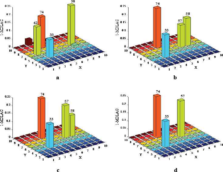
Results of damage identification using the present IDE with noise 3% for Scenario 2. (a) 2 mode shapes; (b) 4 mode shapes; (c) 5 mode shapes; (d) 6 mode shapes.
| Mutation strategy | Scenario 1 | Scenario 2 | |||||||
|---|---|---|---|---|---|---|---|---|---|
| NSA | f | x1 | x2 | NSA | f | x1 | x2 | x3 | |
| DE [28] | 7644 | 0.1035 | 0.4055 | 0.5956 | 13956 | 0.1056 | 0.1457 | 0.1976 | 0.2511 |
| IDE [28] | 2688 | 0.1035 | 0.4053 | 0.5957 | 3464 | 0.1056 | 0.1458 | 0.1975 | 0.2511 |
| IDE (present (2 modes)) | 4008 | 0.8997 | 0.2574 | 0.6000 | 4851 | 0.8747 | 0.1133 | 0 | 0.1945 |
| IDE (present (4 modes)) | 4170 | 0.9002 | 0.3338 | 0.5955 | 4925 | 0.9107 | 0.1428 | 0.1391 | 0.2488 |
| IDE (present (5 modes)) | 3892 | 0.9045 | 0.3911 | 0.5971 | 4340 | 0.9221 | 0.1495 | 0.2009 | 0.2489 |
| IDE (present (6 modes)) | 4000 | 0.9054 | 0.3994 | 0.6000 | 4295 | 0.9162 | 0.1524 | 0.2024 | 0.2507 |
where, NSA=average number of structural analysis; NS= number of stages; f =the value of objective function; for scenario 1: x1=damage extent of element 37, x2=damage extent of element 47; for scenario 2: x1=damage extent of element 33, x2=damage extent of element 57 and x3=damage extent of element 74.
Statistical results of damage identification for the square composite plate in the case of noise-free
As shown in Figs. 9, 10 and Table 7, the present IDE with 6 modes has better results in terms of accuracy than the present IDE with 2, 4, 5 modes and the DE in Ref. 28. Fig. 9 indicates that the false damage elements of element 32 using 2 and 4 modes and element 100 using 5 modes are detected. Fig. 10 illustrates that the false damage elements of element 58 and 62 are identified but the true damage element 57 is lost in Fig. 10 (a), and element 58 using 4 and 5 modes are wrongly detected in Figs. 10 (a) and (b). Therefore, it can be concluded that the more the number of the modes is, the higher the precision of identification is. For the computing time, the present IDE with different modes is faster than the DE in Ref. 28. However, due to the Ref. 28 only include the quantification of damage severities, the present IDE still shows superior computing performance.
6. Conclusions
In this work, a multi-stage method based on multiple damage location assurance criterion and an improved differential evolution algorithm is presented for damage identification of civil engineering structures. The computational cost of damage identification process is reduced as far as possible by the suitable selection of damage range and filtering threshold in defferent computational stages. The IDE is proposed by a new adaptive scaling factor with a segmented function used in the mutaion operator of the basic differential evolution (DE) algorithm. The numerical examples for a continuous beam and a square composite plate are performed to show the effectiveness and robustness of the present method. In these examples, different damage scenarios are considered by reducing the stiffness of these elements as well as the effect of noise is investigated. The results demonstrated that the multi-stage method based on MDLAC and the IDE in each stage is effective for both locating and quantifying the damage regardless of the effect of noise. For computational accuracy and cost, the present IDE with more mode shapes has better performance than the basic DE and DE in Ref. 28.
Acknowledgements
This work was supported by the “985 Project” of Jilin University, the National High Technology Research and Development Program of China and the National Natural Science Foundation of China (Nos.51378236). The financial support is gratefully acknowledged.
References
Cite this article
TY  - JOUR
AU  - Chunli Wu
AU  - Hanbing Liu
AU  - Xuxi Qin
AU  - Guojin Tan
AU  - Zhengwei Gu
PY  - 2017
DA  - 2017/07/19
TI  - Multi-stage method to identify structural damage using multiple damage location assurance criterion and an improved differential evolution algorithm
JO  - International Journal of Computational Intelligence Systems
SP  - 1066
EP  - 1081
VL  - 10
IS  - 1
SN  - 1875-6883
UR  - https://doi.org/10.2991/ijcis.2017.10.1.71
DO  - 10.2991/ijcis.2017.10.1.71
ID  - Wu2017
ER  -