
Intelligent Centroid Localization Based on Fuzzy Logic and Genetic Algorithm
- DOI
- 10.2991/ijcis.2017.10.1.70How to use a DOI?
- Keywords
- Intelligent Centroid Localization; RSSI; Localization Error; Fuzzy Logic; Genetic Algorithm
- Abstract
For many of the applications in which wireless sensor networks are used, it is important to know from which nodes or what location useful information is acquired. The Global Positioning System (GPS) is conventionally used to determine location. However, GPS systems are not ideal for many applications due to their excessive power consumption and high cost. As an alternative to GPS, distance and location can be estimated through the usage of at least 3 nodes with known locations. Received Signal Strength Indication (RSSI) is the simplest and most inexpensive technique used to determine distance and location, and is a standard feature on every sensor. However, RSSI can be affected by noise and environmental obstacles. For this reason, it is difficult to set up a mathematical model for RSSI. This paper presents a conversion of the Centroid Localization (CL) method in determining the location of a sensor of unknown location to the Intelligent Centroid Localization (ICL) Method. Fuzzy logic and genetic algorithm are employed in the ICL method. RSSI values measured by anchor nodes are applied as inputs to the fuzzy system in the ICL developed. Anchor nodes have been assigned weight values to increase the effect of high-value RSSI nodes in positioning. Therefore the fuzzy system’s output is defined as weight (w). The base values of the fuzzy system’s output membership functions are adjusted using genetic algorithm to minimize location error. Toward observing the performance of the proposed ICL, comparisons with the both Centroid Localization method and APIT (Approximate Point In Triangle) algorithm have been provided. The localization error has been reduced to minimum levels.
- Copyright
- © 2017, the Authors. Published by Atlantis Press.
- Open Access
- This is an open access article under the CC BY-NC license (http://creativecommons.org/licences/by-nc/4.0/).
1. Introduction
Location determination is a significant problem in wireless sensor networking. The Global Positioning System (GPS) can be used to determine location. However, GPS systems are not ideal for many applications due to their excessive power consumption and high cost. As an alternative to GPS, distance and location can be estimated through the usage of at least 3 nodes with known locations. Simply put, the localization problem in sensor networks is the determination of the location of sensors physically scattered into different places in the network through the usage of sensors with known locations. Sensor location is accomplished in two steps. The first step is distance estimation. In this step, a signal exchange between sensors is used to estimate the distances between them.
The second step is location estimation. In this step, sensor coordinates are estimated using methods such as distance-based triangulation, using multiple planes, etc. In most applications, the data collected from the wireless sensors must be associated with the relevant locations of the sensor nodes to make the data meaningful and useful. So, it is important to determine the sensor location with an accurate algorithm. In recent years many algorithms have been developed to estimate distance and location1,2,3,4. It is possible to examine such algorithms developed for location estimation in two categories, Range-Free and Range-Based, as shown in Figure.1 1.
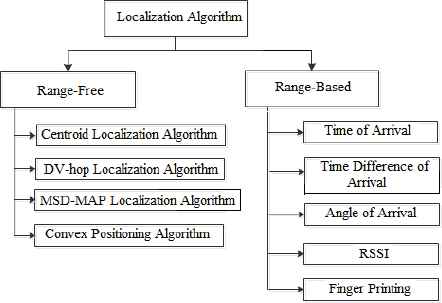
Localization Algorithms
Localization algorithms based on range-free techniques obtain the location of unknown nodes according to information provided by anchor nodes3,4. Radio coverage membership: An anchor node detects whether an unknown node is in its radio coverage. Using this information, the system can estimate the unknown node location. Number of hops to an anchor node: If there is no connectivity with an anchor node, the unknown node can estimate its location using knowledge of the number of hops to every anchor node.
Attempts to estimate location by using the proportions of RF signals to distance (signal strength / time of arrival) in the Range-Based algorithms. In the time of arrival (TOA) method, locations are calculated based on a signal’s travel time information5. By sending out continuous signals successively, location is estimated using the time difference between arrivals of the signals. In the time difference of arrival (TDOA) method, location is calculated by measuring time elapsed between signal transmission and response receipt in the signal exchange between two sensors6. In the angle of arrival (AOA) method, location is calculated using the incoming signal’s angle information7,8. Anchor nodes send messages including their angles and proximity to other anchor nodes in their vicinity. Nodes receiving these messages calculate their own locations using the distance and angle information provided. In order to calculate location, information must be received from at least two anchor nodes. Specific equipment is needed for this technique. The Received Signal Strength Indication (RSSI) method is based on the principle that the power of the signal beamed out of a sensor is inversely proportional to the square of its distance9. In the fingerprint method, previous RSSI measurements are stored a database10. Sensor location is estimated by comparing old RSSI values in the database with newly measured RSSI values.
In recent years, soft techniques have been used to develop both range-based and range-free localization estimation methods11,12,13,14,15,16. In ref.11 was proposed a trust-based secure sensor localization scheme using a neural network. Simulation results showed that the proposed TSLS scheme can improve the accuracy of sensor localization. In Ref.12 was proposed two soft computing localization techniques based on range based localization. These techniques are Neural Fuzzy Inference System and Artificial neural Network. These techniques have been successfully tested in both indoor and outdoor environments. The results indicated that techniques were more convenient than the other algorithms adopted to work in terms of distance estimation accuracy. Methods developed using Fuzzy Type-2 and Fuzzy C-Means have been performed effective, robust and accurate location detection in the indoor environment13,14. One of the traditional methods, FingerPrint, has been developed with a hybrid approach in the Ref.17. NN and GA were used in this approach. In this study, the position error is reduced to minimum levels by increasing the number of anchors. In Ref.18 has been presented an optimization algorithm of improved DV-HOP based on genetic algorithm The simulation results have been compared with the conventional DV-HOP algorithm. The results showed that higher location accuracy has been obtained.
Besides these studies, there are studies using classical localization algorithms. One of the conventional methods that can be used to estimate location is the Centroid Localization method, which cannot accurately determine location3. The necessity of a Weighted Centroid Localization algorithm in minimizing location error has been demonstrated in Ref.19. In order to increase the effect of anchor nodes that are close to nodes of unknown location in positioning, the weight parameter (w) has been used in Ref.19. The main logic behind this algorithm is that the shorter the distance between the anchor node and unknown node, the higher the weight parameter. The most important point to take into consideration here is the manner in which the weights are determined. The Adaptive-WCL20 and Modified-WCL21 algorithms are proposed to determine the correct weights. In Ref.19, weights have been determined using the LQI (Link Quality Indicator) measured by anchor nodes. After determining a nominal LQI value, the difference between this value and the LQI value by measured anchor nodes have been used as weight. In Ref.22, to determine the distance between the anchor node and the unknown node, two different parameters (α, β), known as adaptivity degree, have been used. Location estimation has been conducted according to the changes in these two parameters in the case the unknown node moves away from or draws closer to the anchor node. In this paper, the mathematical expressions of these two parameters and the algorithm used for location estimation have been defined in depth.
Soft computing algorithms are proposed as a solution for correct determination of the aforementioned weights22,23,26. While calculating the location of a sensor of unknown location using nodes with known locations, the weight parameter is used to increase the impact of the node with the highest RSSI value on location determination. Structures based on fuzzy logic have been developed to calculate these weights22,24. The biggest problem with these systems is that they are created using specialist knowledge. Accurately determining these weights using fuzzy logic-based systems means that the sensor location is also calculated accurately.
In proposed fuzzy logic-based system, RSSI is the system input and the system output is the weights (w). In such a system, it is important to set up the relationship between RSSI and w correctly. The correct identification of this relationship and therefore the computation of the appropriate weights turn into an optimization problem. To solve this problem, a structure based on fuzzy logic and genetic algorithm is developed in this paper. For this reason, the Centroid Localization method and APIT Algorithm are explained in paper’s second section. Fuzzy logic and genetic algorithm definitions are provided in the third section to explain the Intelligent Centroid Localization method. In the fourth section, the implementation of Intelligent Centroid Localization and the gradual processes of the proposed system are detailed. In the fifth section, simulation results are provided. In conclusion, ICL method assessments are provided.
2. Centroid Localization Algorithm and APIT Algorithm
2.1. Centroid Localization Algorithm
One of the conventional methods that can be used in location estimation is the Centroid Localization method. In this algorithm, the locations of sensor nodes with unknown locations are determined by using the coordinates of at least 3 anchor nodes. The main advantages of this method are, the similarity between the calculations for each node and a lesser processing load. Despite that, the method has a disadvantage in that it calculates the coordinates of sensors with unknown locations with high error values. Figure 2 shows the calculation of location for a sensor of unknown location using the Centroid Localization algorithm by utilizing 3 anchor sensors and the error value.
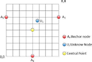
Central Point Calculation
Where, CPx and CPy represent the x and y coordinates of the Central Point. Ux and Uy are the actual location coordinates of the sensor. The estimated location error of a sensor is calculated as follows according to equation 2.1.
It is important to minimize error to correctly determine location. To do this, a weight (w) value proportional to the distance between every anchor node and the unknown location node should be determined. Equation 2.2 gives the location computation of the sensor of unknown location considering the effect of weights. Where, xest and yest are the estimated coordinates of a sensor.
2.2. APIT Algorithm
Approximate Point In Triangle (APIT) is an area-based range-free localization scheme. In this algorithm, triangular regions containing the sensor node is created by anchor nodes. The intersection of triangular regions is a polygonal region. The center point of this polygonal region is the coordinates of the unknown sensor to be estimated. In this algorithm, the location error is dependent on the number of anchor nodes, that is, the number of triangular regions. The APIT algorithm can be broken down into four steps27. In the first step, the nearest anchor nodes to the unknown sensor are determined according to the RSSI signal power. In the second step, triangular regions are created by using anchor nodes. In the third step, Polygonal region is created by triangular regions including sensor of unknown location. Finally, the center point of the polygonal region is calculated. The center point is location of sensor whose location unknown. The location error is computed as in the equation.1. Figure.3 shows the polygonal region and center point determined by 4 anchor nodes for APIT algorithm.
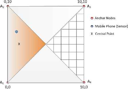
APIT algorithm and center point
3. Fuzzy Logic And Genetic Algorithm
3.1. Fuzzy Logic
Fuzzy logic is a soft computing method that is used for nonlinear, complex situations that are difficult to model and involve ambiguous or uncertain information. As in human logic, it also works according to interval values like very long, long to medium, short, too short, etc. The information in fuzzy logic comprises linguistic expressions (big, small, slightly, etc.). Everything in fuzzy logic is shown with a certain value between the interval [0,1]. The fuzzy inference process is carried out according to rules defined between linguistic expressions. Fuzzy logic is substantially convenient for systems in which a mathematical model is very difficult to obtain. Figure 4 below demonstrates fuzzy logic structure.
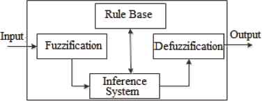
Fuzzy Logic
Fuzzification is the process of converting a system input into symbolic, linguistic attributes. Input values are assigned to linguistic variables such as small, the smallest, etc., by determining where the fuzzy cluster/clusters that input information belong and their membership degree. After a model’s input and output variables are determined, the relation between input and output is designated using the rules in the rule base. If X and Y are system inputs and Z is output, then the following rule determines the fuzzy value of output Z according to the inputs X and Y: if X=x and Y =y then Z = z. Fuzzified inputs and the inference unit using the rules stored in the rule base process the input data and generate a fuzzy output. This output has to be converted from a fuzzy value into a real value since it will be used in the real world (in a real system). This process is referred to as defuzzification.
3.2. Genetic Algorithm
Genetic Algorithm (GA) is a global research technique based on natural selection and genetic rules. GA generates continuously improving results in a manner similar to natural selection. In order to perform this operation, fitness functions specifying the goodness of chromosomes and operators like cross-over and mutation are used28. A GA pseudo code is given in Algorithm 1.
| Begin |
| Initialize Population; |
| Evaluate Population; |
| While not (Termination Criteria Reached) do |
| Begin |
| Select Solutions for Next Population; |
| Perform Cross-over and Mutation |
| Evaluate Population; |
| End; |
| End; |
Simple Genetic Algorithm( )
The first step in GA is to generate an initial population to be used for GA process. The general trend in initial population generation is the random generation of chromosomes. If the solution type can be estimated or gene ranges are known, the solution process must be accelerated by generating an initial population with known parameters. In each generation, the applied operators are as follows: Parent chromosomes are selected with respect to their success criteria (fitness values). Cross-over applied to these parent chromosomes and new chromosomes are obtained. The newly yielded chromosomes are evaluated (computing of fitness values). The GA process must continue either up to a specified number of generations or until the desired success is obtained in at least one chromosome.
4. Experimental Setup and Intelligent Centroid Localization Algorithm
4.1. Experimental Setup
An area of 10x10 m2 has been selected for location detection in the indoor environment. Anchor nodes are placed in each corner of this environment that can measure temperature. The temperature sensor is on the MSP430 controller. The measured temperature information is transmitted to the mobile phone in the environment via the Bluetooth HC-06 module. In this experimental environment the mobile phone is the sensor or node whose location we attempted to estimate. The MSP430 controller has 10 pin GPIO, internal temperature sensor, 8 channel 10 bit ADC, 2KB flash and 128 Bytes RAM. It is designed for wireless serial communication applications. The MSP430 controller allows communication at 2.4GHz frequency that is supported Bluetooth 2.0. Figure 5 shows the MSP430 controller, HC-06 Bluetooth module and application environment.
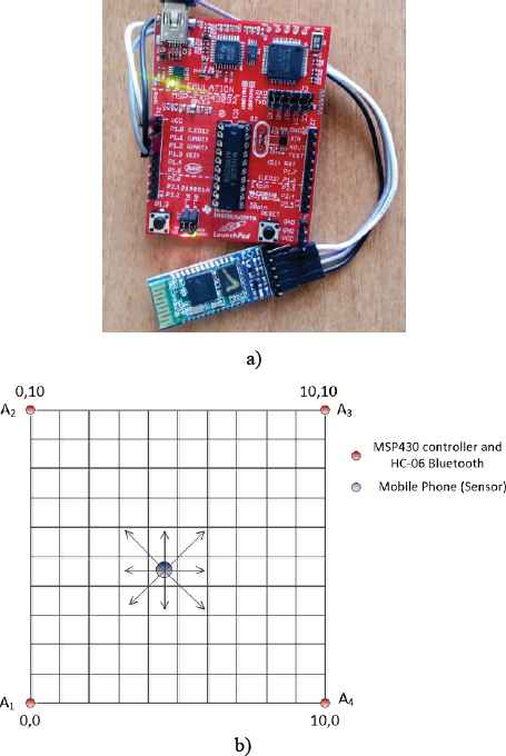
a) MSP430 Controller and HC-06 Bluetooth Module b) Application Environment29
With Android-based software, the mobile phone can measure the RSSI value of incoming signal from anchor sensor via Bluetooth. In order to determine the location of the mobile phone from the RSSI values obtained from four different sensors in the environment, the three highest values are used for location estimation. Figure 6 shows the mobile phone measurement of the RSSI value obtained from an anchor sensor.
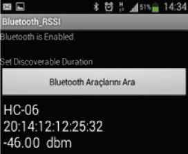
RSSI measurement with mobile phone
4.2. Intelligent Centroid Localization Algorithm
The accuracy of the Centroid Localization algorithm depends on the correct selection of weights (w1,w2…wn) involved in the equation 2.2. We propose the ICL method to accurately determine these weights. The Intelligent Centroid Localization system proposed to determine appropriate weights consists of a 2-step process. The first step is a process that determines the appropriate weights by employing fuzzy logic and genetic algorithms. The second step of the process is testing the system. In the first system process, the steps required to determine the appropriate weights are as follows:
Step.1. Determine 10 random nodes of unknown location (There should be at least 3 nodes of known location in the wireless sensor network).
Step.2. Obtain RSSI values from 3 neighboring anchor nodes for each of the nodes.
Step.3. Randomly determine the RSSI, which is the fuzzy logic input and output, and base values of the weight (w) membership functions.
Step.4. Enter the RSSI values measured by three anchor nodes (for each sensor of unknown location) as inputs to the fuzzy system.
Step.5. Calculate the weights for each node of unknown location corresponding to the RSSI values from the fuzzy system output.
Step.6. Calculate the fitness function to assess whether the sensor locations have been accurately determined.
Step.7. Terminate if fitness function is minimal.
Step.8. Update the fuzzy system output membership function (weight (w)) base values according to the genetic algorithm process.
Step.9. Return to the 4th step.
Step.10. Terminate.
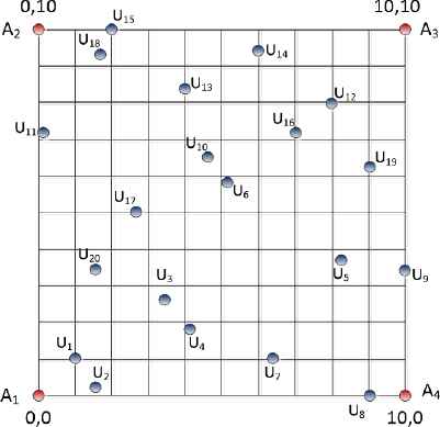
A wireless network environment such as that shown in Figure 7 is considered as a reference. Figure 7 depicts a square with 10 m edges with 4 nodes of known location on each corner. The RSSI values for 10 randomly selected nodes of unknown location on this platform are given in Table.1.
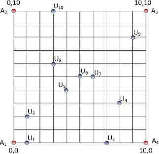
The platform determined for simulation
| Node Number | RSSIA1 | RSSIA2 | RSSIA3 | RSSIA4 |
|---|---|---|---|---|
| U1(1,0) | -40 | -75 | -73 | |
| U2(7,0) | -70 | - | -76 | -57 |
| U3(1,2) | -52 | -72 | - | -74 |
| U4(8,3) | -73 | - | -70 | -60 |
| U5(4,4) | -66 | -70 | - | -70 |
| U6(5,5) | - | -70 | -70 | -70 |
| U7(6,5) | - | -71 | -68 | -68 |
| U8(3,6) | -69 | -65 | -72 | - |
| U9(9,8) | - | -74 | -52 | -72 |
| U10(3,10) | -76 | -57 | -70 | - |
Actual values and RSSI values for each node
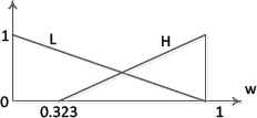
The RSSI value measured by the sensor of known location is the input to the fuzzy system. As shown in Figure 8, the RSSI membership function is converted into two triangular fuzzy sets, labeled Low (L) and High (H). The RSSI input has base values of RSSImin(-80dbm) and RSSImax(-40dbm). The output membership function is the weight and its base values changes over the interval 0 to 1. The weight membership function is also converted into two triangular fuzzy sets, labeled Low (L) and High (H). The rules utilized in the system are created according to the reasoning explained below. If the RSSI measured by the anchor node is high, it can be said that the sensor of unknown location is close to the anchor node. In this situation, that anchor node’s impact on Localization should be greater while determining the sensor of unknown location’s position. The opposite is also true; therefore rules can be established as follows:
Rule 1: if RSSI is high, then w is high
Rule2: if RSSI is low, then w is low
It is an optimization problem to determine the most appropriate w value corresponding to each RSSI value. It is appropriate to employ genetic algorithm to solve this problem. The first step of the genetic process is to form an initial population with different base values. Figure.8 shows the fuzzy system’s randomly chosen input and output membership functions.

Fuzzy system’s input and output membership functions
The first step of the genetic algorithm process is to initialize the population and code the individuals. Every individual or chromosome in the population contains the base values of B1 and B2. Since the base values B1 and B2 base are in the interval [0,1], B1 and B2 must be coded after they are normalized. To do so, every chromosome is coded using the binary number system. A total of 14 bits are used to represent chromosomes in the population with the binary system. The first 7 of 14 bits denote the B1 base value and the last 7 bits denote the B2 base value. The maximum value that each base value can achieve in coding is 1111111. However, the base values must be normalized base to be equalized with the maximum value, 1111111. Equation 4.1 can be utilized toward this end17.
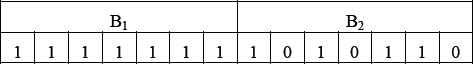
Demonstration of the example chromosome
Bmax =1, Bmin =0, in this case the weight membership function’s base values B1 and B2 will be;
Output membership function for an example chromosome.
After generating the initial population of the genetic algorithm for the different chromosomes shown in Figure 9, the processes of cross-over, mutation and population generation for the next generation are carried out according to the Algorithm 1. Obtaining accurate base values depends on the decided fitness function. To do this, a minimization of the difference between the estimated and actual locations of n sensors such that their locations can be estimated can be used as a fitness function. The fitness function can be established as shown in Equation 4.2.
The genetic algorithm process is carried out until the fitness function decreases to the minimum or a desired value. If the desired fitness level has not been attained, the process is carried out by updating the fuzzy system’s output, the weight membership function base values (which generate a new population). In this paper, the fitness function value is calculated using the obtained weights from a total of 10 nodes. In accordance with the genetic algorithm process, the output membership function base values (B1 and B2) have been changed until the desired fitness function is reached. The fitness function depends on the location of the used 10 nodes. The value of the fitness function for different nodes can change. The obtained minimum fitness value for the nodes specified in Table 1 is 12.55 m. The fuzzy logic output function’s base values at the instance of genetic algorithm process termination are obtained as in Figure 11.
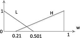
The most suitable output membership function
Figure 12 and Table 2 show the change in location error obtained with the proposed ICL method relative to both the Centroid Localization method and APIT algorithm for 10 nodes. In the Centroid Localization method and APIT algorithm the total error are calculated as 21.91 and 26.43 respectively. Average errors are 2.191 and 2.643 in meters, while in the ICL method total error is 12.55 and the average error is 1.255, also in meters.
| Node Number | Centroid Localization | APIT | ICL |
|---|---|---|---|
| U1(1,0) | 3.13 | 4.52 | 1.42 |
| U2(7,0) | 2.78 | 3.54 | 1.55 |
| U3(1,2) | 1.79 | 3.14 | 0.74 |
| U4(8,3) | 1.38 | 2.13 | 0.14 |
| U5(4,4) | 1.89 | 1.49 | 1.38 |
| U6(5,5) | 2.35 | 1.69 | 2.34 |
| U7(6,5) | 1.79 | 0.74 | 1.83 |
| U8(3,6) | 0.74 | 1.38 | 0.85 |
| U9(9,8) | 2.7 | 4.08 | 0.76 |
| U10(3,10) | 3.36 | 3.72 | 1.54 |
Location error calculated in meters according to the Centroid Localization, APIT and ICL methods
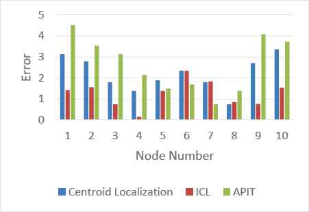
Centroid Localization, APIT and Intelligent Localization method variations in error
5. Simulation Results
As mentioned above, the second part of the process is to test the system. In this process, testing determines whether the locations of 20 nodes randomly placed into the environment in Figure 13 were accurately determined.
Test Envirenment
The location information obtained through the ICL method has been inspected according to Centroid Localization and APIT algorithm. Table 3 shows the calculated error values according to Centroid Localization, APIT algorithm and Intelligent Centroid Localization. According to the Centroid Localization method and APIT algorithm, total errors are obtained 45.804 m and 55.07 m respectively. According to the ICL method, the total error is 19.735 m. Centroid Localization methot and APIT algorithm the average errors are 2.29 m and 2.75 m respectively while According to the ICL method average error is 0.986 m. Figure.14 illustrates the error variation according to all of the methods. With ICL method, even as the calculation load increases, location error is reduced by approximately 57% and 65% as compared to the Centroid Localization method and APIT algorithm.

Error variation according to CL, APIT and ICL
| Node(x,y) | ErrorCL | ErrorICL | ErrorAPIT |
|---|---|---|---|
| (1,1) | 3.299 | 1.173 | 4.01 |
| (1.6,0.2) | 2.58 | 1.378 | 4.58 |
| (3.4,2.6) | 0.736 | 0.368 | 1.26 |
| (4.1,1.9) | 1.625 | 0.591 | 0.94 |
| (8.3,3.8) | 1.699 | 0.501 | 1.85 |
| (5.1,5.9) | 1.743 | 1.844 | 1.99 |
| (7.4,1) | 2.445 | 0.75 | 3.27 |
| (9,0) | 4.068 | 1.76 | 5.11 |
| (10,3.4) | 3.334 | 1.558 | 3.56 |
| (4.6,6.5) | 1.277 | 1.111 | 0.18 |
| (0.1,7.2) | 3.276 | 1.424 | 3.62 |
| (8,8) | 1.887 | 0.382 | 3.51 |
| (4,8.3) | 1.764 | 0.559 | 1.76 |
| (6,9.4) | 2.813 | 1.061 | 3.17 |
| (2,10) | 3.59 | 1.498 | 3.43 |
| (7,7.1) | 0.547 | 0.368 | 3.28 |
| (2.6,5) | 1.821 | 1.164 | 0.34 |
| (1.7,9.3) | 3.099 | 1.035 | 4.72 |
| (9,6.3) | 2.362 | 0.71 | 2.85 |
| (1.5,3.5) | 1.84 | 0.5 | 1.64 |
Error changes to 20 different nodes
6. Conclusion
Determining distance and location is a significant problem in wireless sensor networking. Over time, in parallel to technological developments, significant improvements in localization systems are taking place and studies are progressing. This paper has presented the Intelligent Centroid Localization method for localization. The disadvantage of the ICL method is computational complexity. The advantage is that the location error is reduced with respect to CL and APIT. With this method, even as the calculation load increases, location error is reduced by approximately 57% and 65% as compared to the Centroid Localization method and APIT algorithm. Although the proposed system does not yield accurate localization, it is open to further development. The success of the ICL method depends on the membership functions, base value of the membership functions, the fitness function, rules and the number of fuzzy sets. The base values of the fuzzy RSSI inputs used in the system can be adjusted to obtain more accurate results. In addition, the manner in which RSSI and weight membership function utilization of more than 2 fuzzy clusters (low-high) impacts location error can be explored. As another proposal, the effect of using LQI together with RSSI to address location error could be examined as opposed to using RSSI alone in location estimation.
References
Cite this article
TY  - JOUR
AU  - Taner Tuncer
PY  - 2017
DA  - 2017/07/07
TI  - Intelligent Centroid Localization Based on Fuzzy Logic and Genetic Algorithm
JO  - International Journal of Computational Intelligence Systems
SP  - 1056
EP  - 1065
VL  - 10
IS  - 1
SN  - 1875-6883
UR  - https://doi.org/10.2991/ijcis.2017.10.1.70
DO  - 10.2991/ijcis.2017.10.1.70
ID  - Tuncer2017
ER  -