
Structure Evolution Based Optimization Algorithm for Low Pass IIR Digital Filter Design
- DOI
- 10.2991/ijcis.2017.10.1.69How to use a DOI?
- Keywords
- structure evolution; genetic algorithm; digital filter design; linear phase
- Abstract
Digital filters are generally designed by identifying the transfer functions. Most researches are focused on the goal of approaching the desired frequency response, and take less additional consideration of structure characteristics which can greatly affect the performance of the digital filter. This paper proposes a structure-evolution based optimization algorithm (SEOA) which allows the integrated consideration of structure issues and frequency response specifications in design stage. The method generates digital filter structures by a structurally automatic-generation algorithm (SAGA) which can randomly generate and effectively represent digital structures. The structures, seen as chromosomes, are evolved over genetic algorithm (GA) for the search of the optimal solution in structure space. They are evaluated according to the mean squared error (MSE) between the designed and the desired frequency responses. Simulation results validate that the algorithm designs diversified structures of digital filters and they meet target frequency specifications and structure constraints tightly. It is a promising way for optimized and automated design of digital filters.
- Copyright
- © 2017, the Authors. Published by Atlantis Press.
- Open Access
- This is an open access article under the CC BY-NC license (http://creativecommons.org/licences/by-nc/4.0/).
1. Introduction
The low pass digital filter is a key component in modern digital systems 1,2 which is characterized by the strong ability of signal processing. Filter design is a process of synthesis and implementation. The designed filter is expected to meet some given constraints, such as the magnitude response, the phase, etc. From a mathematical point of view, the problem of filter design is a constrained minimization problem.3 Design of digital filters generally is focused on the identification of the transfer function.1 Structures synthesis of the digital filter is the process of converting the transfer function into a digital filter structure.4
The performance of a real digital filter can be strongly affected by the errors from the frequency response in the identification stage and the structure characteristics in structure synthesis stage. While the transfer function may be optimal for a desired frequency response in the identification stage, it is not globally optimal because of the lack of the consideration of the structure constraints (system scale, component types, connection modes). In fact, the structure constraints are difficult to be reflected in the transfer function. Moreover, digital filter synthesis is usually based on some fixed structures or hand-designed ones, such as frequency sampling, lattice and improved lattice.1,2,5 Those structures maybe fit the target response very well for some special tasks, but the lack of diversity of structures results in less flexibility for a random task. The overall optimization of identification and synthesis for digital filters is still a unresolved problem.
The aim of this paper is to develop a new design method for digital filters. In the method, the identification and the synthesis stages are merged so that all constraints take effects, and structure space of digital filters are greatly expanded through a structure-evolution technique.
There is a considerable amount of literatures on digital filter design. Most studies have only focused on the identification of a transfer function. Some literatures report the structure synthesis methods for digital filters, but none of the researchers has addressed the question of overall optimization of the identification and the synthesis. The following is a survey of the traditional and the state-of-the-art technology on digital filter design and implementation.
1.1. Traditional identification methods
Traditional design methods attempt to identify the transfer function or the unit impulse response. They are classified into two kinds according to the filter patterns. One kind is for finite impulse response (FIR) digital filters and the other is for infinite impulse response (IIR) digital filters.1,2
The window method 3,6 is the most commonly used method for the design of FIR digital filters. In the method, it is pre-requisite to get the impulse response from the desired frequency response, and then the impulse response is multiplied by a window function. The method is efficient and fast, but the truncation of the impulse response results in large ripples in pass band and stop band 6,7 in the frequency domain.
Another popular method for FIR digital filter design is the frequency sampling method.1,2,6 In the method, the desired frequency response is sampled and then is transformed to the corresponding finite impulse response by means of an inverse discrete fourier transform (IDFT). The main weakness of the method is that the filter frequency response has a finite error between the samples.3,8
Parks-McClellan method 9 in practice is particularly easy. The goal of the algorithm is to minimize the error in the pass and the stop bands by utilizing the Chebyshev approximation. It uses Remez exchange algorithm 3,6 to find an optimal equiripple set of coefficients. Through a iterate process, it finds the set of coefficients that minimize the maximum deviation from the desired frequency response. This method depends on fixed or floating point implementation, numerical accuracy as well as the filter order.7
IIR filters are designed using different methods. One of the most commonly used methods is based on the reference analog prototype filter.2 The filter design process starts with specifications and requirements of the desirable IIR filter. A type of reference analog prototype filters to be used, such as Chebyshev and Butterworth, is specified according to the specifications. After the design of the analog filter, the analog filter is converted to the digital filter. The most commonly used converting methods are bilinear transformation,10 impulse invariance,11 and pole-zero matching method.12 The bilinear transformation can convert a transfer function of an analog filter to that of a digital filter with a nonlinear mapping. It preserves the stability and minimum-phase property of the analog filter, only with a drawback of the nonlinear frequency mapping. In contrast to this method, impulse invariance provides a solution in time domain, in which the impulse response of the analog system is sampled to produce the impulse response of the digital system. In this method, aliasing will occur without a band-limited measure, including aliasing below the Nyquist frequency to the extent that the analog filter’s response is nonzero above that frequency. Pole-zero matching method works by mapping all poles and zeros of the s-plane to the z-plane locations z = esT, for a sampling interval T. Weighted least-squares design for digital IIR filters in Ref. 13 makes denominator polynomial decomposed as a cascade of a few second-order factors and a higher order factor. The factors are updated in each iteration meanwhile taking the stability into account. It is concerned on computational efficiency and design accuracy. Two reweighted minimax phase error algorithms are proposed in Ref. 14 to design nearly linear-phase IIR digital filters when the pass, stop and transition bands satisfy their specifications.
1.2. Evolutionary identification methods
In recent years, evolutionary algorithms have been used to design FIR or IIR digital filters. They are concerned on the problem of coefficient optimization of the transfer function.
The commonly used algorithm for IIR or FIR filter design is Genetic Algorithm (GA).15 It codes the coefficients of the transfer function. By the evolution process, GA is used to search the optimal coefficients. However, its disadvantages are lack of good local search ability and premature convergence.16
Particle Swarm Optimization (PSO) algorithm 17 has been used in the digital IIR filter design. The parameters of filter are real coded as a particle and then the swarm represents all the candidate solutions. PSO is quite easy for implementation and outperforms GA in many practical applications. However, as the particles in PSO only search in a finite sampling space, it also lacks the ability to jump out of the local optima when solving complex multi-modal tasks.16
Ant colony optimisation (ACO) 18 imitates the social behavior of real ant colonies. It may occasionally be trapped into local stagnation or premature convergence resulting in a low optimizing precision or even failure.19
Some evolutionary algorithms are sensitive on the control parameters or the initial states. Seeker optimization algorithm (SOA) 20 simulates the act of human searching and has been widely developed for system identification. Nonetheless, the performance of SOA is affected by its parameters, and it could not easily escape from premature convergence.19 Differential evolutionary (DE) 21 algorithm has been used for digital IIR filter design. The problem of DE algorithm is that it is sensitive to the choice of its control parameters. Simulated Annealing (SA) algorithm 22 in the digital IIR filter design is usually sensitive to its starting point of the search, and often requires much more number of function evaluations to converge to the global optima.
In order to further optimize the solution, some researchers recently proposed improved or new methods. Hybrid genetic algorithm (HGA) 7 introduces a self-adaptive management of the balance between diversity and elitism during the genetic life. Only some promising reference chromosomes are submitted to a local optimization procedure. The hybridization and the involved mechanisms afford the GA great flexibility for the specific area of FIR filter design. DE with a new wavelet mutation 23 is proposed for designing linear phase FIR filters, and the result shows remarkable improvements in filter performance. A hybrid algorithm 24 of fitness based adaptive DE and PSO is efficient for designing linear phase FIR filters. Different versions of PSOs and GAs were compared for FIR filter design in Ref. 25, it is pointed out that self-tuning strategies are very important for the improvement of their efficiency. Harmony Search (HS) algorithm 26 is applied for the identification of IIR filters, and excellent results are obtained for the global optimization and rapid convergence. An opposition-based HS (OHS) algorithm 27 is applied to the solution of the FIR filter design problem, yielding optimal filter coefficients. Another new optimization method named gravitational search algorithm (GSA) 28 is adopted for designing optimal linear phase FIR band pass and band stop digital filters. GSA guarantees the exploitation step of the algorithm and it is apparently free from premature convergence. GSA with Wavelet Mutation (GSAWM) is proposed in Ref. 29 for the design of IIR digital filters. RPSODE (Random PSO in hybrid with DE) 30 is used for the design of linear phase low pass and high pass FIR filters, which produce better magnitude response and convergence speed than PSO, DE and PSODE.
Cat Swarm Optimization (CSO) 31 is used for optimal linear phase FIR filter design. The algorithm is generated by observing the behaviour of cats. Every cat has its own position composed of M dimensions, velocities for each dimension, a fitness value which represents the accommodation of the cat to the fitness function, and a flag to identify whether the cat is in seeking mode or tracing mode. The final solution would be the best position of one of the cats. A Two-Stage ensemble Memetic Algorithm (TSMA) 32 framework is proposed for IIR filter design. It attempt to synthesize the strengths of the evolutionary global search and local search techniques. In a competition way, the best local search technique is adopted to obtain good initial state. Inheriting the good information of the first stage, the second stage is to implement effective adaptive memetic algorithm (MA) to pursue high-quality solution.
Other works are focused on certain aspects of the performance of digital filters or that of design methods. An improvement in code of GA appears in Ref. 33, where a canonic-signed-digit (CSD) coded GA is proposed to improve the precision of FIR filter coefficients. Through restraining poles in a disk D(α,r) within the unit disk, it is reported that DE has a great help to improve the robustness of IIR filters.34
DE has also been explored to search the impulse response coefficients of the FIR filter in the form of sum of power of two (SPT) in order to avoid the multipliers during design process.35 A new local search operator enhanced multi-objective evolutionary algorithm (LS-MOEA) 36 is specifically proposed for multi-objective optimization problems, with equal consideration of magnitude response, linear phase and the order of structure. A kind of DE variants with a controllable probabilistic (CPDE) population size is proposed in Ref. 37. It considers the convergence speed and the computational cost simultaneously by partially increasing or declining individuals according to fitness diversities.
1.3. Structure implementation of digital filters
From a practical point of view, it is desired to implement a filter with such a structure that not only has a good capability against the finite word length (FWL) errors and no overflow oscillation, but also has a very low implementation complexity.5 In some particular occasions, reliability, stability, redundancy, power, delay or scale of system are considerable in structure design. Although there are an unlimited number of equivalent filter structures realizing a given transfer function,37 those often used forms are limited, such as frequency sampling and lattice form.1 The structure designed by existing methods is less considered about its diversity.
A flexible structure synthesis method for IIR digital filters is presented based on a desirable transfer function.4 In the method, digital filter structures are represented as S-expressions with subroutines, which are written directly from the set of difference equations. The method is used to design low-coefficient sensitivity filter structure and the low-output roundoff noise filter structure. It is able to create many different structures, but the adder is limited to two inputs in the method.
Lattice structures are applied in a wide range of areas, owning to their excellent FWL properties.38,39 A new class of lattice-based digital filter structures is derived in Ref. 5. Each stage of the lattice structure can take any one of four elementary lattice structures, which are created by the authors. Consequently, possible combinations for the lattice structure are increased. The optimal structure problem has been formulated in terms of minimizing the signal power ratio. Although the lattice structure grows in quantity, the structure in fact is still restricted by the connection of lattice structures.
A synthesis method for the implementation of a special filter of low-complexity variable fractional-delay (VFD) filters has been proposed.40 The structure designed by the method is efficient only for VFD digital filters.
A real implementation of the evolvable hardware system 41 is presented to autonomously generate digital processing circuits on the field programmable gate array (FPGA), which is implemented on an array of processing elements (PEs). The connections between PEs are fixed, and only the PE’s function may be changed. The diversity of the structures of digital filters will be limited in this situation.
1.4. The process and characteristics of the proposed algorithm
In this paper, we propose a structure evolution based optimization algorithm (SEOA) to design low pass IIR digital filter structures. The algorithm aims to deal with the issues of both the structure and its frequency response. It comes with three major parts. The first part is representation and automatic generation of digital filter structures. A structurally automatic-generation algorithm (SAGA) is proposed for randomly generating digital structures. It is based on circuit-constructing robot (cc-bot),42 which is an automation for generating analog circuits based on instruction sequences. SAGA inherits the merits of cc-bot, such as the ability to work with GA and structural diversity. The second parts is the method of structure evolution. GA is used to evolving structures by searching filter structure space. Structures, coded by instruction sequences, are seen as chromosomes. The chromosomes are involved by GA for the search of the optimal solution in structure space. The last part is the restriction and evaluation of structures. With applying structure restraints, structures are evaluated by means of MSE between the designed and the desired frequency responses. SEOA has been validated by designing and implementing digital filters. Encouraging results are obtained. The designed filters show such excellent characteristics as diversified structures, validated structure constraints and well approximating frequency responses.
To our knowledge, the similar work has not been reported. SEOA is characterized by the following outstanding properties. 1. The algorithm can be used for the integerated optimization of digital filters, because both of structure issues (such as component specifications and system scale) and filer response specifications (such as magnitude and phase) can be combined into consideration in the design period. 2. When satisfying structure constraints and matching the desired frequency response tightly, the structures are greatly diversified. SEOA is able to provide novel designs that human designers have never envisioned. 3. There is no limits to the desired response, whether it is continuous or discrete, with a formula or not.
This paper is organised as follows: Section 2 formulates structure design problem and presents SEOA. Section 3 tests the filter performance of both structures and frequency responses in simulation. Finally, Section 4 concludes this paper.
2. Problem formulation and algorithm description
2.1. Problem formulation
A filter structure indicates a filter network, including component specifications, connection modes and system scale. For a linear time invariant (LTI) digital system,1 there are three types of logical components, the adder, the multiplier and the delay element. They are connected with each other to form various network topologies. The structure of a digital filter is often characterized by a set of difference equations. Every difference equation indicates an input-output relation on a network node. The transfer function of the digital filter can be acquired by solving the equations.
The low pass IIR digital filter is widely used in many industry fields. The target magnitude response is set the ideal low pass filter as equation (1).
The structure of a digital filter is coded by an instruction sequence Sk in this paper. Assuming an evaluation function is denoted by Fe, it is used to evaluate the magnitude response of a filter structure. The smaller the return value of Fe is, the better the structure is. We use a simple structure constraint of the limitation of system scale. ‖Sk‖ denotes the system scale, which is limited in the range between Clow and Chigh. The system scale is the sum of the delay elements and the multipliers.
In evaluation function Fe, the structure Sk needs to be transformed into H(K) for error estimates, where H(K) is sampled from the magnitude frequency response of the structure. The transformation from Sk to H(K) is introduced in section 2.2.6. At last, the weighted mean-squared-error (MSE) is used to evaluate filter performance shown in
2.2. Algorithm description
2.2.1. Overview of the algorithm
The proposed algorithm designs digital filter structures based on GA. GA has the potential of obtaining high performance.25 The structure is evolved by GA and is evaluated by a fitness function. Along with structure evolution, the fitness of structures decrease until the algorithm reaches a maximum generation or the fitness satisfies given conditions. The following are the stages of the algorithm.
2.2.2. The generation and code of digital structures
Crossover in GA is difficult to be applied to circuit individuals, because correct circuits may become wrong when they cross with each other. Cc-bot aims to generate analog circuits and it works well together with GA. It can make crossover well done between two circuits, and the resulting circuits are always correct. It starts with the input node of a system and advances to append components one by one. The beginning node is also called the active node, which will switch into another position of the circuit in the generating process. A new component has five connection selections to link itself to the circuit. One terminal of the component is linked to the active node. The other terminal is linked to the starting node, a prior node, the ground node, the ending node (the output node of the filter), and a new node. Only the new node has a privilege to become the active node. Other four connections don’t change the position of the active node. New randomly-selected components are appended onto the circuit until all components are used up, and a new circuit is generated. Compared with 2-terminal components, 3-terminal components, such as triodes, have more connecting ways and are more complicated.
But cc-bot is not suitable to generate digital structures, because digital filters consist of digital components different from analog components. Digital components in a digital LTI filter include the delay element, the multiplier and the adder. In these types of components, the adder is a particular one. It has more than 2 terminals, in which more than one of them are input terminals and the other is the output terminal. The number of the input terminals are variable. In the circuit-generating process, when an adder is appended to the circuit, its terminals may increased in quantity as components appended later may be linked to the adder. The variable number of terminals will bring complexity in generation, coding and crossover.
Another problem is that cc-bot does’t need to consider signal direction in analog circuits. In digital structures, every terminal of components must have its signal direction and these directions can’t collide with each other. For example, if one branch bears more than one components, the components must have the same signal direction.
A. The structure generation
We design a structurally automatic-generation algorithm (SAGA) for digital filters. In the algorithm, the structure starts with one node that is the input node of system, and grows by attaching components to it one by one. Newly appended components must link one terminal of itself to the active node. The active node is the unique source of growth for the structure. This ensures that the structure can be represented by an instruction sequence, and cooperate fully with crossover operators in GA.
Components are appended to a structure in four ways. With the input terminal connected to the active node, an added component connects its output terminal to a new node, a previous node, the system input node and the system output node in the structure. The four types of connection are coded as Cnew, Cpre, Cin and Cout. An example is shown in Fig. 1. In the example, a multiplier is added to the structure with two ways of Cnew and Cpre.
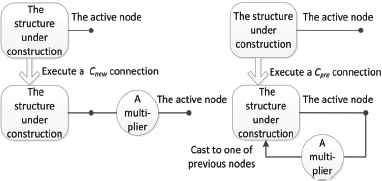
The SAGA algorithm’s connection types: (a) connection to a new node (b) connection to a previous node.
The system input node is the first active node of the structure. The system output node is a node that always exists in the process of structure generation, so that one terminal of the newly appended component can be linked to it.
Two types of components are prepared to generate a structure, i.e. the delay element and the multiplier, denoted separately by Td and Tm. Each of them has two terminals and any kind of the four connections can be applied to them. The adder, however, has variable number of terminals. It is complex to connect the adder to the structure. A easy way is to take the adder into account after the structure is finished, because the four connections will naturally produce adders when feedback branches are attached to a previous node. The number of terminals of every adder is fixed on that time. Those nodes with more than one inputs become adders.
A special case is the connection of the last component to the structure. The connection is constrained to Cout, because it gives no guarantee that previous certain node has been connected to the output terminal of system. After the last connection, system’s output terminal is definitely linked to the structure. Consider a node of the structure, there are di signals flowing into it and do signals flowing out from it. The direction constraint of digital structures can be
In order to always generate valid structures, every node must satisfy formula 5. In fact, when Cnew open up a new position for the active node, it already produces an input to the active node. The active node is inevitable to advance to the next position by Cnew or to the output node of system by Cout. Whether Cnew or Cout is selected, each of them produces an output from the active node, which guarantees that formula 5 holds for every node.
Finally, the selections of connection type, component type and component value are all random. Each type of connections takes the probability of 0.25, each component type takes 0.5. The previous node connected by Cpre is randomly selected in the range from the first node to the active node.
B. The structure code
In the initial stage of GA, the first generation of structures is generated. They can’t be directly operated by generic operators unless they are coded. We code a structure by an instruction sequence. Every component appended on the structure is driven by an instruction. The instruction, denoted as Tcon|Vi|Vo|Pc|Tcom, consists of five parts. Tcon denotes connection type of the component. Vi and Vo are the nodes that the input and output terminals of the appended component are linked to. Tcom indicates the component type, i.e. the delay element or the multiplier. Pc is the component’s parameter.
An instruction sequence reflects a process to generate a structure. The structure can reappear when following the instruction sequence. It is used to represent the chromosome in GA. Obviously, the number of components will affect the length of chromosome. More components bring more computation and longer time to converge. But less components may not be able to achieve a fitting structure. The Table 2.2.6 shows a 7-component instruction sequence, and Fig. 2 is the structure created by the sequence.
| ID | Tcon | Vi | Vo | Pc | Tcom |
|---|---|---|---|---|---|
| 1 | Cnew | N1 | N2 | − | Td |
| 2 | Cin | N2 | N1 | 2 | Tm |
| 3 | Cout | N2 | N0 | 0.5 | Tm |
| 4 | Cnew | N2 | N3 | − | Td |
| 5 | Cpre | N3 | N2 | 0.3 | Tm |
| 6 | Cin | N3 | N1 | −0.1 | Tm |
| 7 | Cout | N3 | N0 | 1 | Tm |
An example for the instruction sequence.
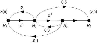
The instruction sequence and the generated signal flow graph (SFG).
The sequence includes 7 instructions in a single-input-single-output (SISO) filter. Active nodes in the process of generation are created one by one, numbered by Ni incrementally. The first active node, i.e. the input node of the filter, is numbered by 1. The output node of the filter is numbered by 0 because the total of nodes are unknown before the structure is completed. The delay element takes unit delay and hence needs no parameters. The final structure includes 5 multipliers, 2 unit delay elements and 3 adders.
2.2.3. Crossover stage
We randomly select some chromosomes by crossover rate (CR). Every chromosome is represented by an instruction sequence. The single-point crossover is adopted. The crossing point is randomly selected at a position between any two instructions of the instruction sequence. A maximum number of components is needed. Or the components in some structures may increase exponentially in number. On the contrary, a too simple structure is also inappropriate in performance. So the crossing point must satisfy the condition that resulting chromosomes are confined within a given range in length.
For example, a 20-instruction-length chromosome crosses with a 15-instruction-length chromosome with a length range of [5,25] in Fig. 3. P2 has a crossing point at 5. The crossing point of P1 is valid at 13. But it is invalid at 18, because the resulting sequence of C1 succeeds upper bound in length.
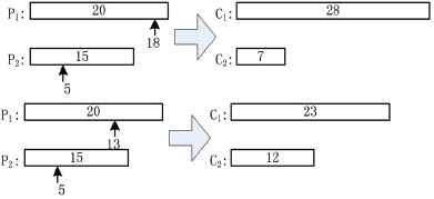
Crossover between two filter structures.
Crossover brings a gap or overlap of the identified number of the node between the first and the second parts of the child chromosome. The problem will result in invalidation of the instruction sequence and the structure. In order to enable the validity of the child chromosome, reclaimed numbers for active nodes (Vi) of the second part are used. The numbers restart from the number of the last active node from the first part. The identified number of Vo remains unchanged for the three connection types of Cnew, Cin and Cout, and is randomly changed within the number range of the first part for Cpre.
2.2.4. Mutation stage
In mutation stage, we randomly select some chromosomes by mutation rate (MR). These selected chromosomes mutated in a particular way. Every chromosome of them will be replaced by a newly created chromosome. The new chromosome has the same length with its predecessor. The mutation method brings more changes in mutation stage than the single instruction mutation which only mutates an instruction of the chromosome.
2.2.5. Selection stage
In selection stage, the elite chromosomes will be elected from the current generation of the chromosomes. The current generation consist of Ps father chromosomes, Pc and Pm child chromosomes. The father chromosomes come from the previous generation, while Pc and Pm child chromosomes are produced separately by the crossover and mutation operators in the current generation from these Ps father chromosomes. These chromosomes are sorted by their fitness. The Ps chromosomes with smaller fitness will be kept down as next generation of chromosomes.
2.2.6. Fitness evaluation
Filter structure is a comprehensive information body. It embodies not only the transfer function but also many other performance function, such as system accumulative error, reliability and FWL effects etc., which go beyond the ability of the transfer function. Basically, component connections, component specifications, system scale, system redundancy, etc. are key factors which comprise a filter structure. Some useful characteristics can be controlled through adjusting filter structure but they can’t be accomplished by the transfer function.
The following is that the amplitude frequency response is derived from the filter structure. We establish an equation between input and output signals on every node as shown in
An instruction sequence represents a structure. The following is the method that derives the system of equations from the instruction sequence. Noticing that the field of Vo in an instruction denotes a collecting node. The collecting node gathers the signal from the output terminal of the component in the instruction. As long as all relative input components are found, we can establish the equation on the node. The following is the algorithm establishing the system of equations from the instruction sequence.
| Require: | |
| The instruction sequence, s; | |
| The length of the instruction sequence, Ls; | |
| Ensure: | |
| The coefficient matrix of the state equation group, ms | |
| 1: | Vmax = s[Ls].Vi + 1 |
| 2: | For i = 1 to Vmax |
| 3: | For j = 1 to Vmax |
| 4: | ms(i, j) ⇐ 0 |
| 5: | EndFor |
| 6: | EndFor |
| 7: | For i = 1 to Ls |
| 8: | If s[i].Vo = 0 |
| 9: | Vc ⇐ Vmax |
| 10: | Else |
| 11: | Vc ⇐ s[i].Vo |
| 12: | EndIf |
| 13: | Vi ⇐ s[i].Vi |
| 14: | If s[i].Tcom refers to a delayer |
| 15: | Pc ⇐ z−1 |
| 16: | Else |
| 17: | Pc ⇐ s[i].Pc |
| 18: | EndIf |
| 19: | ms(Vc,Vi) ⇐ ms(Vc,Vi) + Pc |
| 20: | EndFor |
Figure out the state equation group
The output terminal of system is identified with 0 in the generation of structures. In order to be compatible with matrix operation, it is changed into the total number of nodes in the algorithm, as shown on line 1. The ms is initialized from line 2 to line 6. As a symbolic matrix with size of Vmax * Vmax, its every item is expressed by a polynomial. The matrix is used to record the coefficients of the system of equations. From line 7 to line 20, all instructions in instruction sequence s are traversed. The node linked by the output terminal of a component, is recorded as Vc from line 8 to line 12. The signal comes from the node linked by the input terminal of the component, which is recorded at line 13. From line 14 to line 18, for the delay element, its parameter is z−1; for the multiplier, its parameter is extracted from the current instruction. For all components linked from Vi to Vc, their parameters are summed at line 19. This considers the case that more components than one are in parallel connection between Vi and Vc. Finally, the symbolic matrix ms stores the coefficients of the system of equations.
Typically, the transfer function can be derived from the system of linear equations and the frequency responses from the transfer function. But the transfer function will consume a lot of computation because of many inverse operators of symbolic matrix. It is infeasible in computing transfer functions with large symbolic matrix. In fact, as long as the values of sampling points in the frequency response are figured out, symbolic operations can be transformed into numerical operations, which greatly decreases computation cost of fitness. The steps of fitness computation are listed as follows.
Step 1. Confirm the relation between the transfer function and the filter structure. Through solving the set of linear equations from the structure, the author in Ref. 43 derives
where I is a unit matrix and S is a state vector. S presents the states of all nodes. That’s, S contains output of every node. For instance, S(k) is the output on the kth node. Finally, P denotes a weight vector from system input to any middle node and system output. Considering the structure-generating method, P = {1,0,…} is set up. Therefore, the transfer function of the structure iswhere S(Vmax) denotes the system output and Vmax is the identified number of the output terminal of the system.Step 2. In symbolic matrix ms, eιπi/ns is substituted for z, where ι is imaginary unit. The variable, eιπi/ns, is helpful to get the value of the ith sample of the frequency response with total ns samples. Euler formula is used to translate symbolic matrix ms into plural matrix mp. S, I and P are changed in the same way.
Step 3. The set of plural equations, expressed by mp, is solved by using LUP (LU (Lower Upper) factorization with Partial Pivoting) decomposition, which is the fastest method at present with time complexity
Step 4. The steps 1–3 run in circles until the values of all samples are got. Fitness is computed based on the values and equation (3).
The steps in this subsection are helpful to achieve computation feasibility and decrease time complexity. Its progress is shown in Fig. 4, where the dotted boxes are those steps that are saved.

The progress of computing fitness
2.3. Algorithm analysis
SEOA is quite different from existing methods for digital filter identification and implementation. The methods for the identification of the transfer function are concerned on the optimization of the frequency response. Structure synthesis methods are focused on the structure characteristics based on the given transfer function. SEOA, however, evolves the filter structures by GA, which is a integrated optimization method. The integration brings in better performance of the digital filter than the two stage optimization, where the transfer function may be optimal in the identification but is not sure about its optimization for the structure synthesis. SEOA is compared with the identification methods as follows.
- •
The traditional identification methods for digital filters are simple, fast and easily implemented, but some inherited drawbacks are obvious, such as truncation effect 3,6 and non-linear mapping.10 The evolutionary identification methods try to find the optimal transfer function in coefficient space. In contrast, SEOA does in the structure space. The difference of them is that the former is local optimization due to its unique consideration of the frequency response but SEOA provides more overall optimization of structure constraints and the frequency response. Consequently, SEOA is more efficient towards the implementation of a real digital filter. In addition, SEOA presents diversified structures and the transfer functions can be derived from the structures.
The transfer function doesn’t appear in SEOA and it is implicit in the structure. In reality, the structure contains more information than the transfer function. A comparison of SEOA and structure synthesis methods is listed as following.
- •
- •
SEOA designs more diversified structures than the structure synthesis methods. Unlike structure synthesis methods, SEOA is not limited by a given transfer function. SEOA is able to produce abundant structures through the random selection and connection among components. By contrast, the classical methods have less dynamics of structure topologies due to their relative fixed connection modes of structures. The methods 4 has a strong ability to create structure diversity, and a limit is that the adder is allowed to have only two inputs. In SEOA, however, the adder is permitted to have any number of inputs.
Another kind of structure design methods, such as Ref. 5, 40, firstly design a novel structure and then optimize the structure parameters. The designed structures are characterized by certain fine natures, such as the low signal power ratio 5 and low-complexity implementation.40 The drawbacks of these methods are that the connection mode of the structure is fixed. Compared with this kind of methods, SEOA provides diversified structures some of which show the distinguished characteristic. Several structures designed by SEOA possess such characteristics as sharp transition band and linear passband phase.
3. Simulation results and discussion
In this section, experiments to realize low pass filters are carried out. The parameters are listed in the Table 2.
| Parameter | Value |
|---|---|
| CR | [0.5,1.0] |
| MR | [0.01, 1.0] |
| Population size | 100 |
| Chromosome length | [10,50] |
| Maximum generation | 10000 |
| Seed | [0.0,1.0] |
| Multiplier gain | [−106,106] |
| Sampling rate | 128 |
The parameter settings of the proposed algorithm.
The chromosome length is measured with an instruction as a unit. The maximum generation is set to 10000, which satisfies most tests according to some experiment tries. The random seed is distributed from 0.0 to 1.0, which supports 30 runs for a group of other given parameters. The multiplier gain is confined within the range of [−106,106] in a real number type. Besides, the delay element is set a unit delay with no extra parameter. The target frequency response and the designed frequency response are sampled with 128 points. In other words, the sampling rate is 128 and the sampling interval in the frequency domain is 0.008π. The size of the search space in this simulation can be estimated as the dimensions of a chromosome. A chromosome includes maximum 50 elements and every element has 5 variables to record itself, therefore the search space for a filter in the simulation consists of 250 dimensions.
3.1. Basic design
The target response is an ideal low pass filter with cutoff frequency of π/2. Formula 4 isn’t used just setting w with a fixed value of 1. Filter structures are evolved by SEOA, which are tested by different structure component combination. Filter structures are measured by fitness. Fitness with a smaller value means a better structure. In order to get the satisfied structure, we first explore the important parameters of GA.
Two groups of tests are carried out for the evaluation of the influence of CR and MR on evolution results. The first group is used to judge the influence of MR. In traditional GA, CR is between 0.5 and 1.0,45 and we initially adopt 0.7 for exploring better MR. Fitness in different MR with CR of 0.7 is listed in Table 3 and Table 4. Fitness is given 2 decimal places for simplicity. The MR is distributed in [0.01, 0.09] with step length of 0.01 in Table 3 and [0.1, 1.0] with step length of 0.1 in Table 4. The maximum, the minimum, mean, median, variance and standard deviation of fitness are compared. The smallest mean of fitness is 10.38 with MR of 0.7. The minimum of fitness is 1.01 with MR of 0.5. Another group is use to test the influence of CR. In this group, the MR is fixed to 0.7 because the smallest mean of fitness appears in the position. CR is varied from 0.5 to 1.0 with step length of 0.1, and fitness is compared in Table 5. The smallest mean of fitness is 9.81 with CR of 1.0. Meanwhile, the minimum fitness 0.14 is also under the same CR. Consequently, it is probably more efficient to explore the fitness when MR is 0.7 and CR is 1.0.
| Parameter | MR |
||||||||
|---|---|---|---|---|---|---|---|---|---|
| 0.01 | 0.02 | 0.03 | 0.04 | 0.05 | 0.06 | 0.07 | 0.08 | 0.09 | |
| Max | 22.27 | 22.79 | 24.93 | 24.53 | 25.37 | 24.35 | 23.28 | 20.94 | 22.04 |
| Min | 5.62 | 7.17 | 5.72 | 5.88 | 6.53 | 4.67 | 7.07 | 3.40 | 3.28 |
| Mean | 12.21 | 11.95 | 11.98 | 11.50 | 12.92 | 12.18 | 12.13 | 12.08 | 12.26 |
| Median | 11.35 | 11.87 | 11.91 | 11.05 | 13.25 | 11.08 | 11.91 | 11.82 | 12.67 |
| Variance | 21.70 | 15.63 | 16.29 | 18.32 | 20.96 | 17.83 | 11.74 | 16.34 | 11.15 |
| Std | 4.66 | 3.95 | 4.04 | 4.28 | 4.58 | 4.22 | 3.43 | 4.04 | 3.34 |
The fitness in different MR with CR = 0.7
| Parameter | MR |
|||||||||
|---|---|---|---|---|---|---|---|---|---|---|
| 0.1 | 0.2 | 0.3 | 0.4 | 0.5 | 0.6 | 0.7 | 0.8 | 0.9 | 1.0 | |
| Max | 20.26 | 18.29 | 19.15 | 17.23 | 19.02 | 17.61 | 18.29 | 17.50 | 17.05 | 15.33 |
| Min | 2.34 | 6.79 | 5.90 | 6.28 | 1.01 | 3.95 | 2.60 | 3.70 | 5.92 | 5.09 |
| Mean | 12.56 | 11.91 | 11.48 | 10.86 | 11.10 | 11.15 | 10.38 | 11.8 | 11.04 | 10.65 |
| Median | 11.94 | 11.83 | 10.61 | 10.19 | 11.01 | 11.18 | 10.04 | 12.03 | 10.79 | 11.09 |
| Variance | 14.40 | 11.74 | 11.37 | 9.79 | 12.64 | 10.27 | 15.09 | 10.93 | 9.57 | 8.75 |
| Std | 3.79 | 3.43 | 3.37 | 3.13 | 3.55 | 3.2 | 3.88 | 3.31 | 3.09 | 2.96 |
The fitness in different MR with CR = 0.7
| Parameter | CR |
|||||
|---|---|---|---|---|---|---|
| 0.5 | 0.6 | 0.7 | 0.8 | 0.9 | 1.0 | |
| Max | 17.57 | 17.53 | 18.29 | 16.96 | 17.10 | 15.94 |
| Min | 5.40 | 5.20 | 2.60 | 5.39 | 4.28 | 0.14 |
| Mean | 11.86 | 11.33 | 10.38 | 11.41 | 10.37 | 9.81 |
| Median | 11.93 | 10.90 | 10.04 | 11.88 | 9.62 | 10.13 |
| Variance | 8.71 | 9.28 | 15.09 | 9.89 | 11.40 | 10.28 |
| Std | 2.95 | 3.05 | 3.88 | 3.15 | 3.38 | 3.21 |
The fitness in different CR with MR = 0.7
The fitness evolutionary curve under the condition that MR is 0.7 and CR is 1.0, is shown as Fig 5. The maximum, minimum and mean of the fitness on the kth generations of 30 runs are separately computed. Three curves with k = 1,2,…,10000 are gotten. The mean decreases greatly from 49.481 of the 1st generation to 13.362 of the 500th generation, producing a 73% decline. The minimum fitness decreases 74% from 24.068 to 6.335 within the first 200 generation. The best fitness converges near the 5000th generation.
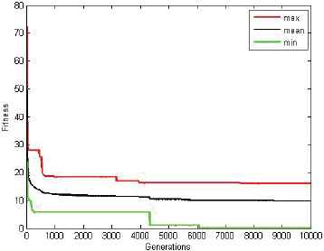
The fitness evolutionary curve with MR=0.7 and CR=1.0 for 30 runs.
The frequency responses with least components are shown as Fig. 6. The total of components is 52, including 2 adders, 27 delay elements and 23 multipliers. The pass band has a small ripple, the transition band has a narrow width and the order of the filter is 9. The stop band attenuate to -14 dB. The frequency responses with least multipliers are shown in Fig. 7. It has a wider transition band about 0.2π, and a smooth pass band and stop band. The attenuation of the stop band reaches -25 dB. The structure contains 5 adders, 32 delay elements and 18 multipliers. Both of the two tests are the result of nonlinear phase. The result shows that the performance of filters is influenced by the structure size of component quantity. Multipliers brings in a more effect on the transition band.
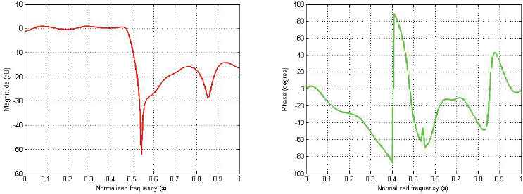
The magnitude and phase frequency response with the least components
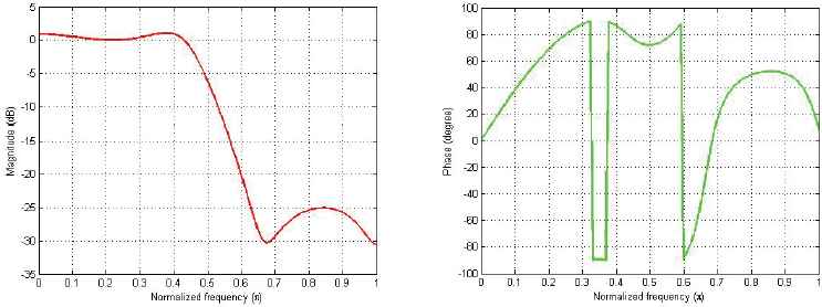
The magnitude and phase frequency response with the least multipliers
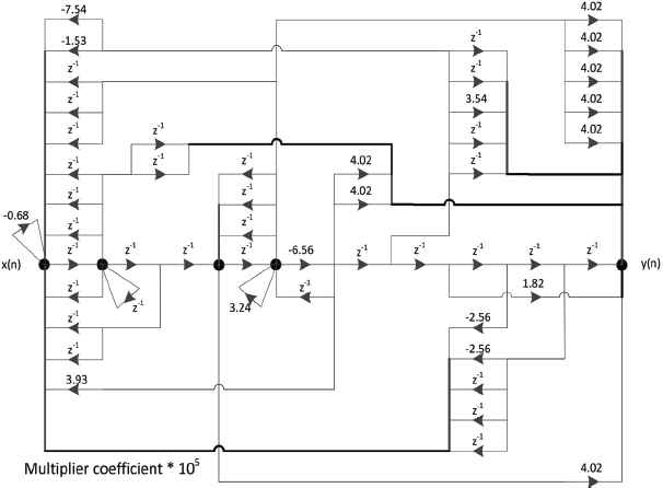
The structure of Fig. 7 is shown in Fig. 11. In the structure, multiplier gain is given 2 decimal places in an exponent form. The solid circle is denoted as adders, arrows with a note ”z−1” are delay elements and other arrows with a floating point number are multipliers. A thin line in the structure indicates a single wire and a thick line indicates a bundle of wires. Intersections in the graph are not adders except solid circles. Delay elements and multipliers are randomly generated and connected, and the total is equal to the upper bound of chromosome length. But adders are naturally produced from the resulting structure. x(n) and y(n) are the input and the output of the system separately. The structure allows self loops, such as those at the 1st, 2nd, and 4th adders from left to right.
3.2. Design of the filter with the sharp transition band and the linear passband phase
In order to strength the transition band, formula 4 is used to weigh the different part of the frequency response. The w is a linear function which creates a 3 times weight at π/2 than that at 0 or π. The weight function makes the fitness more suitable to get a better transition band.
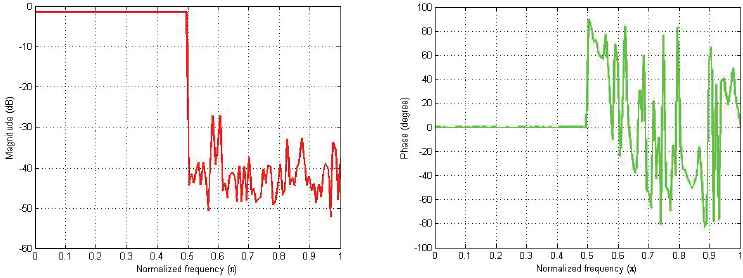
The designed digital filter with the minimum fitness of 0.14, produces a frequency response as shown in Fig. 8 and its structure in Fig. 12. The magnitude frequency response shows a flat pass band and a sharp transition band. The pass band ripple is 5.09 * 10−4 and the width of transition band is a sampling interval of 0.008π. The order of the designed filter is 9. The structure of the designed filter is shown as Fig. 12. In the structure, there are 9 adders, 28 delay elements and 22 multipliers. The structure uses the most components of 59 among 30 runs. In the test, a sharp transition band is obtained with a very flat pass band. The phase response in pass band is piecewise linear, which shapes a sawtooth wave.
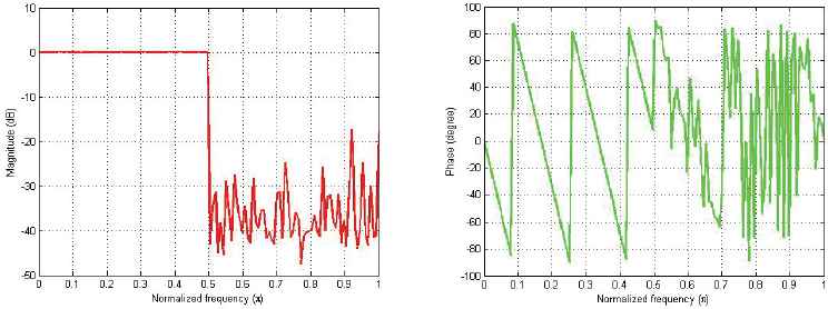
The magnitude and phase frequency response with the best fitness and most components
An approximately linear phase characteristic is obtained on pass band in Fig. 9. Its phase on pass band is almost equal to zero with mean of −5.8 * 10−3 degrees and variance of 2.0 * 10−3. Its pass band ripple is 3.60 *10−3, the width of the transition band is 0.08π, and the maximum attenuation of the stop band reaches -24.37 dB. The order of the filter is 9. Another result is shown in Fig. 10 and its structure is in Fig. 13. In Fig. 10, the phase on pass band holds the mean of 8.56 * 10−4 degrees and variance of 1.21 * 10−4. Its pass band ripple is 7.81*10−4, the width of the transition band is 0.08π, and the maximum attenuation of the stop band reaches -27.22 dB. The order of the designed filter is 6. In Fig. 13, there are 7 adders, 24 delay elements and 26 multipliers. The test shows that SOEA designs the low pass IIR digital filter of sharp transition band and the linear passband phase with low orders less than 10.
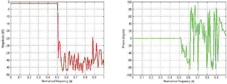
The magnitude and phase frequency response with the approximately linear phase characteristic on pass band (μθ = −5.8 * 10−3,σθ = 2.0 * 10−3)
The magnitude and phase frequency response with the approximately linear phase characteristic on pass band (μθ = 8.56 * 10−4,σθ = 1.21 * 10−4)
3.3. Compare and discussion
Through comparing the structures in Fig. 11–13, some interesting results can be concluded. First, the structures which are generated by our algorithm is valid. Second, the structures are diversified for implementation of the same frequency response and structure characteristics. Third, the structure is controllable because component specifications, connection modes and component quantity are easily set in our algorithm. The structures in Fig. 11–13 can be simplified, specially in the situation of several parallel delay units or multipliers. But this maybe bring different structure characteristics. The designed structures have practical significance in industry manufactures. The algorithm proposed by this paper offers a overall mechanism which allows to design a filter structure directly to meet the target frequency response.
The structure with the least multipliers
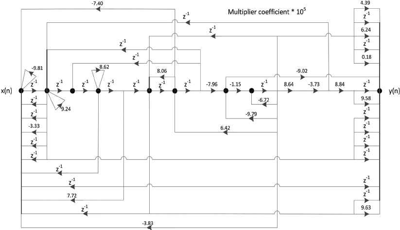
The structure with the best fitness and most components
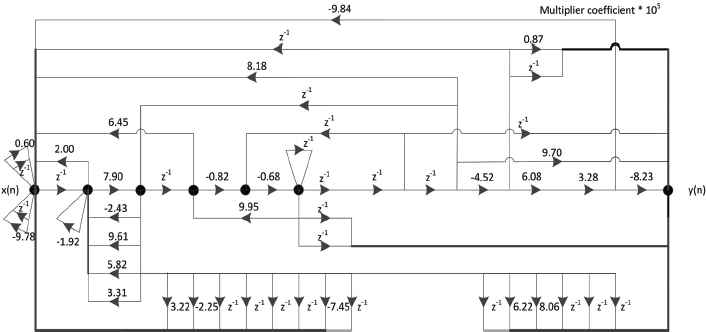
The structure with linear phase characteristics
The pass band ripple and stop band attenuation in different CR with MR = 0.7 are shown in Table 6. The pass band ripple achieves 10−4 and stop band attenuation reaches blow -27 dB. When CR is 0.5, 0.7 and 1.0, the same minimum of fitness is reached and the same structure in structure space is obtained. The structure provides a magnitude frequency response with pass band ripple of 7.81 *10−4 and stop band attenuation of -27.22 dB. The smaller ripple of 5.09 * 10−4 on pass band comes from another solution when CR is equal to 1.0.
| CR | Minimum | Maximum |
|---|---|---|
| pass band ripple | stop band attenuation | |
| 0.5 | 7.81 * 10−4 | -27.22 |
| 0.6 | 5.86 * 10−3 | -8.27 |
| 0.7 | 7.81 * 10−4 | -27.22 |
| 0.8 | 7.74 * 10−2 | -11.28 |
| 0.9 | 9.05 * 10−2 | -10.32 |
| 1.0 | 5.09 * 10−4 | -27.22 |
The comparison of pass band ripple and stop band attenuation in different CR with MR = 0.7.
In our several tests, w plays an important role in optimizing the transition band and the pass band. It is effective to improve different zones of the magnitude response. We set the basic weight to 1 and the maximum to 3, because other values greater than 3 almost overrate the importance at transition band and thereby weaken the other zones. w is set a linear function for a gradually better performance towards the most concerned zone. The non-linear functions are easy to cause the fluctuation of the frequency response. In the result, the filters have not only a proximately linear-phase pass band but also a sharp transition band.
The components involved in structures are classified in accordance with their types. The statistics about component number are listed in Table 7. The MR is equal to 0.7 and CR varies from 0.5 to 1.0. The maximum, the minimum, mean, variance and standard deviation are counted from the data of 30 runs . The upper bound of chromosome length is 50 which is reached at almost all resulting structures. It indicates that a structure produced by more components can perform better.
| CR | Adders | Multipliers | Delay elements | Sum of components |
|---|---|---|---|---|
| 0.5 | 9,2,5.23,4.19,2.05 | 41,11,24.37,41.69,6.46 | 39,9,25.03,41.69,6.46 | 59,40,54.63,11.62,3.41 |
| 0.6 | 8,2,5.77,2.32,1.52 | 35,11,25.60,31.21,5.59 | 39,15,24.30,32.08,5.66 | 58,52,55.67,2.09,1.45 |
| 0.7 | 9,2,5.40,3.21,1.79 | 38,16,27.27,34.48,5.87 | 34,12,22.53,36.46,6.04 | 58,50,55.20,3.96,1.99 |
| 0.8 | 10,3,5.73,3.65,1.91 | 35,18,25.77,24.25,4.92 | 32,15,23.63,24.65,4.97 | 60,43,55.13,8.95,2.99 |
| 0.9 | 13,3,6.00,6.48,2.55 | 37,15,25.63,20.65,4.54 | 35,13,24.27,21.10,4.59 | 63,53,55.90,6.37,2.52 |
| 1.0 | 9,2,6.00,3.24,1.80 | 31,18,25.13,14.33,3.79 | 32,19,24.77,14.81,3.85 | 59,52,55.90,3.20,1.79 |
The general comparison of component number in different CR with MR = 0.7 (data in format: max,min,mean,var,std)
4. Conclusion
This paper proposes a new algorithm to design digital filters based on structural evolution. The algorithm creates filter structures and makes them evolved based on the genetic operators. The method is able to obtain a filter structure with the desirable frequency response. It is helpful to be applied in filter automatic design.
The algorithm provides a new design thought from structure level to target responses. It explores wider structure space than existing methods. The weight function is effective to optimize the magnitude response. The low pass IIR digital filter with the sharp transition band and the linear passband phase is designed in this paper.
The algorithm is concerned on the structure evolution, in which the component parameters are randomly set. In the future work, the optimization of the component parameters is an interesting topic. The proposed algorithm is a promising way for overall optimization and design automation of digital filters.
Acknowledgments
This work was supported by the Foundation of Henan Province, China, with the grant numbers: 15A510018, 15A510019, 12A510002 and 142102210629. This work was also supported by the Foundation of Henan University, China, with the grant numbers: 2008YBZR028 and ZZJJ20140037.
References
Cite this article
TY  - JOUR
AU  - Lijia Chen
AU  - Mingguo Liu
AU  - Jianfeng Yang
AU  - Jing Wu
AU  - Zhen Dai
PY  - 2017
DA  - 2017/07/13
TI  - Structure Evolution Based Optimization Algorithm for Low Pass IIR Digital Filter Design
JO  - International Journal of Computational Intelligence Systems
SP  - 1036
EP  - 1055
VL  - 10
IS  - 1
SN  - 1875-6883
UR  - https://doi.org/10.2991/ijcis.2017.10.1.69
DO  - 10.2991/ijcis.2017.10.1.69
ID  - Chen2017
ER  -