3.1. Prototype structure description

Although prototype classifier techniques in recommender systems are very different, they are based on the same assumptions: (1) structures of prototypes are accuracy, and (2) classifiers are based on nearest neighbour rule. That is to say, (1) a perfect example can be gotten to describe a prototype, and (2) the feature weights are known when deciding the similarity of an unlabelled example. We call these classifiers feature-based prototype classifier. They are not applicable for opaque concepts like social circles’ preferences. In our prototype, we assume the feature space is influenced by items. The differences between two prototypes are reflected by items, not features. We call it item-based prototype classifier (IPC). Firstly, we propose an item-based prototype to describe social circle. In the following paragraphs, the main concepts used in our model are described.

Assuming the recommender system which contains a set of items Item ≔ {u₁, u₂, u₃, ⋯, u_n}, a set of features Fea ≔ {F₁, F₂, F₃, ⋯ F_m} and a set of social circles which is represented as a prototype set Pro ≔ {A₁, A₂, A₃, ⋯, A_h}. A social circle is a labeled prototype A_i which is composed by a subset of items and the memberships of the items belonging to the prototype. So the prototype A_i will be denoted by

The item u_j is also represented as a fuzzy multiset:

Each item u_j is assumed to consist of some features. The feature vector of u_j is Rep(u_j) ≔ {v_j1 v_j2 v_j3 ⋯ v_jm}.

Humans are well known to belong to many associative groups simultaneously, with various levels of affiliation, which is called overlapping groups[15]. Let’s take an example to explain the relations between items and social circles. Junk eaters and healthy eaters compose two social circles. All kinds of food are items. Junk eaters like junk food, but it does not mean that they never buy healthy food. Junk foods are liked by junk eaters, but it does not mean that they never be bought by healthy eaters. Both of these junk food and healthy food have the potential possibility in their shopping baskets, though some are more likely than others. So an item has the relation with all prototypes which was not pointed out by previous literature. The grade of membership μ_ij defines the degree to which each item u_j fits A_i.

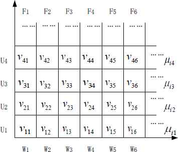
The descriptor can be represented by two 2-dimensional matrices, where x axis is associated to prototypes of the whole descriptor A_i ∈ Pro, and y axis is associated to itemsu_j ∈ Item. Each position (x, y) of the matrix is μ_ij which represents the degree to which each item u_j fits prototype A_i. z axis is associated to feature F_p ∈ Fea. Each position (y, z) of the matrix is v_jp which represents the feature of item u_j . Fig.2. shows the structure used to keep all this information.

Fig.2.

The two 2-dimensionnal matrices of a prototype

If a category is commonly discriminated by features, then decision makers know well the feature’s role in deciding which category the item belongs to. Decision makers also know well the best position in the feature space to represent the category. That is to say, we calculate the distance between a new item and an assumed item whose features best represent the category. But in our problem, the perfect item is not existing. We can only use several items to reflect the differences between two prototypes. The complex relationship of features is hard to tell. So we apply Fig.2. to descript a prototype’s structure.

From function (2), we can see an item can belong to several prototypes. These items reflect the characteristics of a prototype from different aspects. When an unlabeled item needs classification, it should also be represented as a multiset. The prototypicality of a prototype is calculated by aggregating distances of the unlabeled item and the items in the set of the prototype. The prototype whose degree of prototypicality is smaller than the other reflects that this prototype is more suitable to label the unlabeled item.

3.2. Identification of the feature space

When identifying a feature space of a prototype, we need to identify two things: features and features’ weights. There is a feature set Fea ≔ {F₁, F₂, F₃, ⋯ F_m} which composes the elements in the feature space of a prototype. The feature F_p is associated to a group of feature values v_jp (j = 1,2,⋯, n) of item u_j. The importance of feature value v_jp in the group is determined by w_p . An implicit feature weighting is subjective and different for each user. A common feature weighting method based on the Term Frequency-Inverse Document Frequency (TF-IDF) is not good at dealing with multi-valued features. In a more general case, the features can be assessed by multi-valued variables or different domains: numeric, linguistic or nominal, Boolean, etc. [38]. We use information gain to decide the relevance of a feature. We take into account the entropy or amount of information for each feature, the more entropy the more weighting should have. This idea is also used by Barranco et al. [38] to assign weights to features in content-based recommender systems.

Information gain, Gain(Item, F_p) is the measure of the difference in entropy from before to after the set, when Item is split on a feature F_p. In other words, how much uncertainty in Item was reduced after splitting set Item on feature F_p . Information gain can be calculated for each remaining feature.

Now we give the definitions of E(Item) and EE(F_p) in function (3).

There are two characterizing measures related to the weighting vector of an OWA operator. The first one, a measure of orness of the aggregation which is defined as

As more of the total weight moves to the weights at the top we are giving more preference to the larger valued arguments. On the other hand by moving more of the total weight to the bottom we are giving preference to the smaller valued arguments in calculating the OWA aggregation. Larger value of orness(W) indicates the preference for larger argument values. While lower value of orness(W) indicates the preference for smaller argument values [40].

The second one, the classical measure of information uncertainty, dispersion, called Shannon entropy, is defined by

It represents the degree to which the aggregation takes into account all information available in the aggregation, in other words, it measures the average amount of information involved in W.

Here the idea is to find the set of weights, among those with the desired attitudinal character, orness(W), having the largest dispersion. Model(1), suggested by [41] to obtain W, is based on the solution of the following mathematical programming problem:

Model(1)

We require A = orness(W) ∈ [0.5,1] making w_i > w_i+1.

The process of identifying the feature space is as following:

• Step 1. Identify the features in the feature space.

• Step 2. Calculate the information gain for each feature.

• Step 3. Get the preferred sequence of features.

• Step 4. Assign weight to feature F_p according to position in the preferred sequence.

The final identified feature space of all prototypes is described as Fig.3.

Fig.3.

The description of feature space

3.3. Item-based prototype classification process

The fuzzy prototype classification process has three phases. In the preparation phase, we pretreat data set to get a simpler one. This phase is not necessary for all classification process. In the training phase, we construct the feature space for every prototype. The second phase we calculate prototypicality of the unlabeled item to a prototype.

1). preparation phase

As we mentioned in above subsection, diversity of feature values is high, feature values of all items need clustering in order to simplify data and reduce the number of subjects. We use K-means Clustering to group v_jp into {mp1,mp2,⋯,mpa} . So y possible values of the feature F_i are clustered to a (a < y) groups. We calculate the centroid mpl(0<l<a) of the group as the target values of the features. Suppose that we have y sample feature vectors v_1p, v_2p, ⋯, v_yp, and we know that they fall into a compact clusters, a < y. We firstly initiate a centroids at random for each cluster which is presented as mpl(1) . And we assign v_jp into set item_l whose centroid is mpl(1) . The next step is to associate remainder point to the nearest centroid. This algorithm aims at minimizing an objective function. The objective function

Now the feature vector of u_j is Rep(uj)≔{m1j1m2j2m3j3⋯mmjm} , where mpjp is the target value of the feature F_p. v_jp is replaced by mpjp .

2). training phase

In this phase, we obtain a set of items Item: {u₁, u₂, ⋯, u_n}. u_j is represented as function (2). We know its feature values and membership with each prototype. All items can be classified into one of the three subsets Item{Good}kItem{Medium}k and Item{Poor}k to represent a prototype, where Item{Good}k , Item{Medium}k and Item{Poor}k is the corresponding high, medium and low membership degrees respectively.

We use information gain to obtain two 2-dimensional matrices to describe prototype structure and identification the feature space. More details can be seen in subsection 3.1 and 3.2.

3). performance phase

In this phase we classify the unlabeled item to a prototype by calculating the prototypicality. We only know the feature values of the unlabeled item. Each unlabeled item is carried out by finding the closest prototype using a defined distance measure. The distance between prototype A_k is as calculated by function(12) (13).

We use items from Item{Good}k to present prototype A_k.

We can get Gx1,Gx2,⋯,Gxh for every u_x. Gxk reflects the distance between u_x and prototype A_k. Smaller Gxk is, closer u_x is to A_k.

Then u_x is represented as a fuzzy set:

We assign u_x into three subsets Item{Good}a , Item{Medium}b and Item{Poor}c according to Gxi,i=1,2,⋯,h .

1. 1).

   a = i, where Gxi=min k=1,2,3(Gxk)

2. 2).

   c = i, where Gxi=max k=1,2,3(Gxk)

3. 3).

   Otherwise b = i.

3.4. A numerical example

To verify our fuzzy prototype classifier, we choose a fragment of a typical data set—Iris data set in UCI Machine Learning Repository ¹. It has four numerical attributes, three classes, and 150 examples. This data set is for crisp classifications. Every example in the data set completely belongs to one class. But in our model, category is required to be a fuzzy class. Item u_j in our model is represented as a fuzzy multiset:

Before the verification we use FCM function in Matlab ² to generate membership set [μ_ij]_3×150 (see Appendix 2). Iris data set in UCI is reformed to fuzzy class data set which allows the fuzzy prototype model to classify each data example as a certain class. In the reformed Iris data set, the membership μ_ij defines the degree to which each item u_j fits A_i as a category. We assign u_j into three subsets Item{Good}a (which is the good example set of A_a ), Item{Medium}b (which is the medium example set of A_b ) and Item{Poor}c (which is the poor example set of A_c ) according to μ_ij,i = 1,2,3.

1. 1).

   a = i, where μ_ij = max_k=1,2,3(μ_kj)

2. 2).

   c = i, where μ_ij = min_k=1,2,3(μ_kj)

3. 3).

   Otherwise b = i.

The verification is separated into two stages: in the first stage, we use a training set to discover feature space for each prototype; and in the second stage, we use the prediction method to verify the inference of the fuzzy prototype model.

The first stage:

We select ten examples from each set Item{Good}i , i = 1,2,3, to compose the training set at random. Others compose the testing set. The training set contains 30 examples and 4 features.

• Samples 1–10 belong to Item{Good}3 of prototype 3.

• Samples 11-20 belong to Item{Good}2 of prototype 2.

• Samples 21–30 belong to Item{Good}1 of prototype 1.

Feature values are continuous number. Before using the concept of information entropy to find the feature space, we transfer continuous features to discrete features. The 30 sample feature vectors v_1p, v_2p, ⋯, v_30p of F_p are supposed to fall into 3 compact clusters. We use K-means Clustering algorithm to complete the process. The process can be seen in Appendix 2.

Then we construct feature space for corresponding fuzzy prototypes.

1. 1).

   calculate the entropy in the whole training set

   E(Item)=−∑Ai∈Prouj∈Itemp(Ai)log2p(Ai)=1.582

2. 2).

   calculate the expected entropy for the feature F₁

   EE(F1)=∑t=13p(F1t)E(F1t)=0.945

   calculate the Information gain for the feature F₁

   Gain(Item,F1)=0.637

3. 3).

   calculate the expected entropy for the feature F₂

   EE(F2)=∑t=13p(F2t)E(F2t)=1.368

   calculate the Information gain for the feature F₂

   Gain(Item,F2)=0.214

4. 4).

   calculate the expected entropy for the feature F₃

   EE(F3)=∑t=13p(F3t)E(F3t)=0.602

   calculate the Information gain for the feature F₃

   Gain(Item,F3)=0.980

5. 5).

   calculate the expected entropy for the feature F₄

   EE(F4)=∑t=13p(F4t)E(F4t)=0.602

   calculate the Information gain for the feature F₄

   Gain(Item,F4)=0.980Gain(Item,F2)<Gain(Item,F1)<Gain(Item,F3) =Gain(Item,F4)

We get the importance ranking of features

We use model (1) to obtain the optimal weights of the features (assume orness(W) = 0.85 ).

We separate the importance ranking of features into two situations: F₂ ≺ F₁ ≺ F₃ ≺ F₄ and F₂ ≺ F₁ ≺ F₄ ≺ F₃.

The second stage:

We calculate Gxk of u_x in the testing item set to measure the distance between every prototype.

We can get Gx1 , Gx2 and Gx3 for every u_x.

We assign u_x into three subsets Item{Good}a , Item{Medium}b and Item{Poor}c .

Then we give the analysis and comparison of this method. In the first verification, we use partial result in our model to compare the accuracy of classification between our method and Fuzzy K-means Clustering.

The process of Fuzzy K-means Clustering is as follows:

1. 1.

   Use the FCM function in Matlab to generate membership set [μ_ij]_3×150 (see Appendix 2).

2. 2.

   Assign u_x into three subsets Item{Good}a , Item{Medium}b and Item{Poor}c according to membership μ_ix.

   1. 1).

      a = i, where μ_ix = min_k=1,2,3(μ_kx)

   2. 2).

      c = i, where μ_ix = max_k=1,2,3(μ_kx)

   3. 3).

      Otherwise b = i.

IPC method chooses30 examples to form the training set in the preparation phase. The rest examples in [μ_ij]_3×150 form the testing set. So in Table 10, the total number of data examples in the testing set of IPC is 120, while the number of data examples in the testing set of the Fuzzy k-means approach is 150. Since the Fuzzy k-means approach here doesn’t separate the training set and testing set, all examples in Appendix 2 are the data to compare with IPC.

The original Iris data set is the basic of comparison. The accuracy of classification is calculated by function (18)

In our model, u_x is classified to set Item{Good}i according to Gxk . If original Iris data set also classifies it to class i, then we think u_x is successfully classified by our method. In Fuzzy K-means Clustering, u_x is classified to Item{Good}i according to membership μ_ix. If original Iris data set also classifies it to class i, then we think u_x is successfully classified by Fuzzy K-means Clustering. The comparison of the two classification methods is listed in Table 1.

In the second verification, we use the whole result in our model to verify the accuracy of fuzzy classification. We not only verify the accuracy of Item{Good}i , but also Item{Medium}i and Item{Poor}i . The reformed Iris data set is the base of comparison.

The accuracy of Item{Medium}i classification is calculated by function (19)

If reformed Iris data set also classify it to Item{Medium}i according to μ_ix, then we think u_x is successfully classified by our model.

The definition of Accuracy_{Poor} is the same.

The result of the accuracy of fuzzy classification by our model is listed in Table 2.

As a concluding remark, this application shows that:

1. (1)

   The performance of IPC in the accuracy of classification is not poorer than Fuzzy K-means Clustering;

2. (2)

   The performance of IPC in the accuracy of fuzzy classification is also acceptable.

4.1. The descriptor of elements in recommender system

Now we give elements in the recommender system.

1. (1)

   item profile

   We use item features and evaluation as the common representations of a profile. The common representation is defined as following:

   (21)Profile::={ID,Item features,evaluation}

   (22)Item features::={feature 1,feature 2,…,feature n}

   (23)Evaluation::={ score(0−5) }

   “Item feature” is a set of feature values of the item. “Evaluation” provides a preference grade which is a relevant score.

2. (2)

   social circle prototype

   Social circle prototype which is represented as Pro ≔ {A₁, A₂, A₃, ⋯, A_h} . Labeled Prototype, A_i is composed by a subset of items and the membership of the item belongs to the prototype. So a prototype A_i will be denoted by

   (24)Ai=μi1/u1+μi2/u2+⋯+μin/un

   The item u_j is represented as a fuzzy multiset:

   (25)uj=μ1j/A1+μ2j/A2+⋯+μhj/Ah

4.2. Process of the new item recommendation

In the following subsections, we describe the recommendation process. Architecture of the recommendation sees Fig.4.

Fig.4.

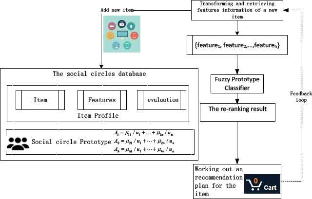
Architecture of the recommendation

Classification phase:

Firstly, we collect the information of the new item u_x. Retrieve the feature values to construct the feature vector {feature₁, feature₂,…,feature_n}. Then compare the feature vector of the new item with u_j feature vector in prototype profile. Use item-based prototype classifier to get Gxk of prototype A_k.

Recommendation plan generation phase:

According to function (26), we can see the new item will be liked by different social circles of users with different favorable degrees. Every social circle has its our effective advertising manner. Then we generate a recommendation plan which contains a set of advertising manners according different social circles.

Our approach is quite different from previous ones. We use Table 3 to show the novelty of our recommendation system.

5.1. Data description and experimental protocol

The beginning of this section starts with an example that clearly demonstrates the new item cold-start problem. We have a RS that includes two sets: users set and items set. When a new item attends into a market, the RS needs to predict the “rating” or “preference” and recommend to the suitable users.

1. a)

   Experimental tools: we adopt Collaborative Filtering algorithms as comparative ones, because these kind algorithms have similar application scenario. We have implemented the proposed approach, NB and MF approaches to predict the “rating” of the new item.

2. b)

   Experimental datasets: To perform experimental evaluations of the proposed ideas we use a benchmark dataset: MovieLens. This dataset (ml-20m) describes 5-star rating and free-text tagging activity from [MovieLens] (http://movielens.org), a movie recommendation service. The data are contained in six files, `genome-scores.csv`, `genome-tags.csv`, `links.csv`, `movies.csv`, `ratings.csv` and `tags.csv`. We extract only positive ratings (rating 5) for training and testing. We choose MovieID 1-20 to compose our training set and randomly choose 16 movies besides these 20 movies to make up the new items testing set. The only requirement of the testing set is that these movies also have rating data by the users in the training set and do not contain features which are not in Table 5. The characteristics of the dataset are summarized in Table 4.

3. c)

   Evaluation indices: we use three widely used measures to compare the recommendation results, namely Mean Reciprocal Rank (MRR), Mean Absolute Error (MAE) and Root Mean Square Error (RMSE).

   • •

     MRR: The Reciprocal Rank (RR) for a recommendation list is the multiplicative inverse of the rank of the first “good” item.

     (27)MRR=1n∑i1ranki

     where n is the number of users who receive recommendations, i.e., the number of recommendation lists, and rank_i is the rank of the first correct item in therecommendation list of user i.

   • •

     MAE and RMSE

     (28)MAE=1n∑u,i|pu,i−ru,i|

     (29)RMSE=1n(pu,i−ru,i)2

     where p_u,i(r_u,i) is the predicted (real)rating of user u for item i.

5.2. Empirical results and discussion

First, we state the processes of the proposed, NB and MF approaches. Then we present the three recommendation results of the approaches. Finally, we give analysis and comparison.

(i) The item-based recommender approach

Users are grouped into several social circles. A social circle is a labeled prototype A_i which is described by a subset of items and the memberships of the items belonging to the prototype. We solve the new item cold-start problem by identifying a feature space of the prototype. Given a new item and its corresponding features, the distance measure between it and a prototype for the new item is computed. Then the ranking of prototypicalities is obtained for this new item.

In the first stage, we use a training set to discover feature space for each group users. Through data arranging, we extract 10 features of these 20 movies from `movies.csv` and obtain Table 5 to describe features. We analyze the data in `ratings.csv` and classify these 20 movies into Group¹ or Group² according to the 5-star rating.Our simplified assumption is that the users giving a same moive 5-starare classified into one group, and a movie liked by one member of the group will be also liked by other member. Then we get Table 6 to describe information of the training set. In Table6, every movie is classified to a group with high membership which is related with the user’s appearance frequency ⁵. We also use this process to obtain the membership of movie in testing set. More the members in Group^p give 5-stars to Movie k, bigger the membership value of the movie to the group is. According to the membership of movie, we give the ranking as the real rating of user i for item k. Higher membership achieves a higher ranking.

MovieId	GroupID	Membership(μj)
1	1	0.95
2	1	0.9
3	2	0.95
4	2	0.8
5	2	0.8
6	1	0.85
7	2	0.8
8	1	0.8
9	2	0.85
10	1	0.85
11	1	0.9
12	1	0.8
13	1	0.9
14	1	0.8
15	1	0.95
16	1	0.8
17	2	0.9
18	1	0.95
19	1	0.95
20	1	0.95

Table 6.

Information of training data

The process as follows:

• Step1. Choose randomly 20 users from 465 users who gave 5 stares to Movie 1-20.

• Step2. User i has a favorite movie set which is U_i = {u_i1u_i2, ⋯ , u_ij}. u_ik is the movie that user i gave 5-stars. Since there are 20 users, there are 20 favorite movie sets, which are U₁, U₂, ⋯ , U₂₀.

• Step3. If the movie u_k is in both U_i and U_j, then we put user i and j in a group. 20 users are grouped in Group¹ or Group².

• Step4. Classify movies into Group¹ or Group² according to the 5-star rating.

• Step5. Set the basic Membership of movie k belonging to Group^p, μ_pk = 0.5.

• Step6. Count the occurrences m of users who gave movie k 5-stars in Group^p.

  (30)μpk=0.5+m×0.05

• Step7. The group Group^p is denoted by

  Groupp=μp1/up1+μp2/up2+⋯+μpn/upn

Calculate the information gain for every feature and get the ranking of features. Use the model (1) to obtain the optimal weights of the features (assume ess(W) = 0.85). The result is described in Table 7.

	F7	F1	F6	F3	F10
EE(Fi)	0.387	0.133	0.116	0.096	0.082
Wi	0.419	0.244	0.142	0.083	0.048
	F9	F2	F5	F4	F8
EE(Fi)	0.059	0.038	0.038	0.025	0.019
Wi	0.028	0.016	0.010	0.006	0.003

Table 7.

Features weights

In the second stage, we use the prediction method to recommend a new movie u_x.We calculate Gxk of the 16 movies to measure the distance between two groups (See Table 8).

(31)Gxk=∑j=1nμj×d(uj,ux)

where u_j ∈ Group^k, k = 1,2.

(32)d(uj,ux)=∑p=110wp·d(vxp,vjp)

NO.(x)	MovieID	Gx1	Gx2	Rank1	Rank2
1	88	0.537	0.685	2	14
2	112	0.373	0.558	1	15
3	185	0.357	0.364	3	11
4	1036	0.357	0.364	3	11
5	2278	0.357	0.364	3	11
6	62	0.501	0.439	10	6
7	318	0.516	0.467	8	7
8	296	0.538	0.513	6	10
9	52	0.603	0.39	14	3
10	34	0.513	0.413	11	5
11	39	0.423	0.238	15	1
12	28	0.602	0.392	12	4
13	36	0.516	0.467	8	7
14	52	0.603	0.390	13	3
15	39	0.423	0.238	15	1
16	514	0.311	0.284	7	9

Table 8.

Results of prediction

In the experiments, we assume

1. (a)

   If Gx1<Gx2 , then we conclude that u_x is more preferenced by group 1. In ‘ratings.csv’, the movie should be given 5 stars by the users in group 1.

2. (b)

   If Gx1>Gx2 , then we conclude that u_x is more preferenced by group 2. In `ratings.csv`, the movie should be given 5 stars by the users in group 2.

We give the Rank_i according to the rules:

IfGx1Gx1+Gx2>Gx2Gx1+Gx2, then Ranki<Rankj;IfGx1Gx1+Gx2=Gx2Gx1+Gx2, then Ranki=Rankj;IfGx1Gx1+Gx2<Gx2Gx1+Gx2, then Ranki>Rankj;

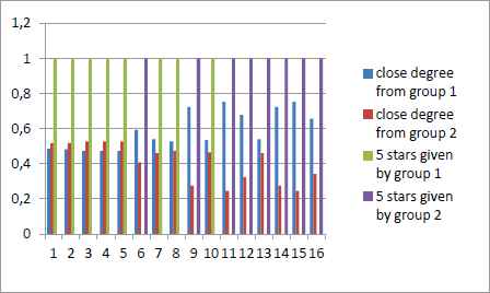
Fig.5. ⁶ presents the calculating results of our experiment.

Fig.5.

Prediction of our recommendation process and original recommendation results of the dataset

(ii) The NB approach and MF approach

In NB approach, recommendations can be done in two ways known as user-based or item-based recommendation. We choose item-based recommendation as the comparative approach. Item-based approaches predict the rating of a user u for a new item based on the ratings of u for items similar to the new one. This idea can be formalized as follows. Denote by Nu(i) the items set rated by user u most similar to item i. The predicted rating of user u for item i is obtained as a weighted average of the ratings given by u to the items of Nu(i) :

(33)rˆui=∑j∈Nu(i)wijruj∑j∈Nu(i)|wij|

where w_i,j reflects the character similarity between i and j. r_uj reflects the preference of user u to item i.

In MF approach, recommendations are made by comparing the properties of the new items to the properties of those items that are known to be liked by representative users(RU). Rating value which measures the preference of the new item liked by RU is calculated in function (34).

(34)rl,j=∑k=1k=Kwk,lvk,j

where r_l,j reflects the item j relation with user u_l. The vector w_*,l is a K-dimensional representation of a user u_l (that is representation of a user u_l in the space of latent features), and the vector v_*,j is a K-dimensional representation of the item i_j (that is representation of an item i_j in the same space of latent features). The set of features is interpreted as a set of representative users. Therefore, value v_k,j expresses preferences of a representativeuser k on the item j and w_k,l– closeness of the user u_l to the representative user k.

We normalize rl,j(rˆu,i) to get rl,j′ (rˆu,i′)

(35)rl,j′=rl,j∑l=1Nrl,j

(36)rˆu,i′=rˆu,i∑l=1Nrˆu,i

We give the Rank_i according to the rules:

If rl,i′>rl,j′, then Ranki<Rankj;If rl,i′=rl,j′, then Ranki=Rankj;If rl,i′<rl,j′, then Ranki>Rankj.

Fig.6. Fig.7. present the calculating results of NB and MF approach experiment.

Fig.6.

Prediction of the NB recommendation process and original recommendation results of the dataset

Fig.7.

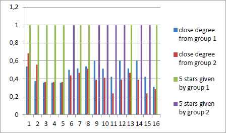
Prediction of the MF recommendation process and original recommendation results of the dataset

Appendix 1.

Given a set of training samples (v_1p, v_2p, ⋯, v_yp), The K-means Clustering [42] algorithm is composed of the following steps:

Appendix 2.