
Analysis of Solar Energy Generation Capacity Using Hesitant Fuzzy Cognitive Maps
- DOI
- 10.2991/ijcis.2017.10.1.76How to use a DOI?
- Keywords
- Fuzzy cognitive maps; hesitant fuzzy sets; renewable energy; solar energy generation
- Abstract
Solar energy is an important and reliable source of energy. Better understanding the concepts and relationships of the factors that affect solar energy generation capacity can enhance the usage of solar energy. This understanding can lead investors and governors in their solar power investments. However, solar power generation process is complicated, and the relations among the factors are vague and hesitant. In this paper, a hesitant fuzzy cognitive map for solar energy generation is developed and used for modeling and analyzing the ambiguous relations. The concepts and the relationships among them are defined by using experts’ opinions. Different scenarios are formed and evaluated with the proposed model.
- Copyright
- © 2017, the Authors. Published by Atlantis Press.
- Open Access
- This is an open access article under the CC BY-NC license (http://creativecommons.org/licences/by-nc/4.0/).
1. Introduction
Growing population and industrialization has been increasing the energy demand throughout the world [1]. Fossil fuels - coal, oil and natural gases- are used as a primary energy source for meeting the majority of the world energy needs. There is a consensus among scholars that conventional energy sources, fossil fuels, have catastrophic damage on the environment by increasing CO2 emission. This emission causes an increase in the surface temperature and stimulating effects such as greenhouse effect, global warming, climate changes and disruption of the food chain [2–4]. Also, fluctuations in the fossil fuel prices that are controlled by a few exporter countries cause an economic inequality among the countries that it leads to the social inequalities among the nations.
Against the environmental and economic damages of the fossil fuels, renewable energy has strongly emerged as an alternative energy source over the last two decades. Renewable energy (e.g. solar, wind, wave, tidal, and geothermal) is the fastest growing energy sources with average 2.6% yearly increase rate [1]. Solar energy has an important place in the renewable energy sources since it is abundant and expansive [5]. Solar can be transformed to energy from simple to high technological methods such as a solar furnace, Photovoltaic (PV), solar pond and Concentrated Solar Power (CSP) [6]. The extensive usage of the solar energy generation system has been increased its demand and usage to reach goals for reducing the greenhouse gas emissions and energy costs [7]. Technological improvements and government subsidies that eliminate its high initial capital costs and support the generation of the solar energy have been developing the interest of the solar systems intensively [8]. Although many countries (Germany, Italy, India, China, Mexico and so on) focus on solar energy generation by incentives and technological supports, solar power production capacity has not reached its deserved potentials [9] yet.
Literature reviews show that the solar energy usage relies on some fundamental factors such as governmental incentives, physical issues, and energy demand and energy provision. Solar energy usage can be increased by defining effective factors, and the causal connections between them. The investors and governors can be conducted toward solar power investments [10]. These factors around the new solar energy generation are dynamic and complex, and the relationships among factors are ambiguous. The aim of the study is to assess the hesitant and causal relationship among the concepts around the capacity of new generated solar energy by using Hesitant Fuzzy Cognitive Maps (HFCMs). HFCMs that are the extension of Fuzzy Cognitive Maps (FCMs) are useful tools for designing model and projecting solar systems in the ambiguous and complex environment. In this paper, a new solar energy generation HFCMs is developed. The factors and causal relationships among them are defined by literature research study and experts’ views [11, 12].
The rest of the paper is organized as follows. Section 2 presents renewable energy, solar energy, and capacity of new generated solar energy factors. Section 3 explains the basic concepts of fuzzy cognitive maps and its application methods. Section 4 is a preliminary part that includes the hesitant fuzzy set (HFS), hesitant fuzzy linguistic term sets (HFLTS), and OWA operations. In Section 5, new developed Hesitant Fuzzy Cognitive Maps (HFCMs) tool is given, and its applications within different scenarios are sampled in Section 6 that gives the proposed new model about the capacity increase and change of solar energy. The study concludes in Section 7 and provides some future views about solar energy and new fuzzy methods.
2. Solar Energy Generation
Energy is a fundamental requirement of human life for the economic and social development of countries by implementing industrialization, transportation, healthcare, education, agriculture, and so on. The energy can be provided by using either a conventional (non-renewable) or renewable energy sources.
Non-renewable (conventional) energy sources use fossil fuels such as coal, oil, natural gas, and petroleum that are carbon based substances. When the fossil fuels are burnt to obtain energy, many environmental damages occur such as air pollution, greenhouse effect, global warming, and depletion of ozone layer, climate change, and acid rain [13]. They are also non-renewable that means they cannot be renewed when used up, and run out one day since their resources are finite. Uncertainties and fluctuations in the global price of the fossil fuels based on the balance between provision and demand cause the economic and social problems on the economies of fossil fuels importing countries [14]. These drawbacks make humankind keep looking for alternative energy sources to produce heat and electricity. However, fossil fuels continue to maintain their existence as an essential part of the energy sources. Despite these disadvantages, they have some advantages such as obtaining a significant amount of energy in a short time, abundant and easy accessibility, high efficiency, stable power generation, easy storage and transportation, and easy construction of their power plants [2, 15].
Renewable energy sources (e.g. the sun, the wind, bioenergy, geothermal, wave, tidal, and hydropower) are sustainable and relevant alternative energy sources against the fossil fuel. They are renewable that means they will never run out in the future. Energy production using renewable energy sources reduces the greenhouse effect since the released air pollution during the production process is low. It also provides cost advantages by means of less maintenance, transmission and production cost [2]. Besides these advantages, there are some disadvantages such as less efficiency based on technological weakness, unstable and unpredictable energy production due to the weather condition, and the requirement of substantial capital cost because their technologies are new and immature, and weakness of scale economy in their sectors.
Improvements in the solar energy technology supported by government incentives and regulations increase the usage of solar energy and enable obtaining economies of scale [20, 21]. From the beginning of the 21st century, countries’ support for renewables includes policy targets, feed-in policies, tendering / public competition bidding, heat obligation and biofuels mandates. For example, Turkey’s investment support policy changed in 2012, and new incentives and regulations were developed to support renewable energies [22]. These developments remove the primary disadvantages of the solar energy for investors and consumers such as initial investment cost, long-term investment gain, and low energy cost and make it attractive as a major alternative energy source against the fossil-based energy sources for meeting the increasing energy need. These policies and regulations increased the global solar generating capacity from 1.3 GW in 2000 to 3.7 GW in 2004, 23 GW in 2009 and 229 GW in 2015 [23].
In this study, we described the factors (Table 1) that affect the capacity of new generated solar energy and causal relations among them for all countries. Causal complex systems [25]. A FCM is a signed and directed graph whose members are called as a node (i.e. concept, factor) and symbolized as Ci. Causal relationships among them are named as an edge (i.e. arc) that represents a weight of direction between two nodes such as node i (Ci) and node j (Cj) and symbolized as wij (Fig. 1). Weight between edges refers the power of the fuzzy causal relationships. The weights are defined by fuzzy relationships are evaluated under the proposed HFCM solar energy generation capacity model. States of the factors in the model are observed at each iteration, and their levels are analyzed in the long term. In this way, the impact of the factors and their causal relationships in the model are verified. New solar energy plant investments can be enhanced by using this model.
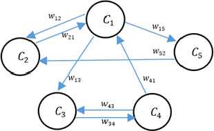
A sample FCM model.
| Factors | Definitions |
|---|---|
| Energy Need (ED) | The demand for energy that is used as an input to carry out human needs such as production, heating transportation [16] . |
| Energy Fee (EF) | The unit fee of the used energy. Increase in conventional energy costs stimulates to increase an inclination towards renewable energy investments at the base of inverse relation [17]. |
| Energy Provision (EP) | Energy is generated for future requirements. The amount of provision can be measured based on the expectation of the energy receiver and/or provider [16]. |
| Non-fossil Fuel Energy Sources (NFES) | Total available energy capacity that is generated by using renewable energy resources (e.g. sun, wind biomass) and controlled by physical (weather, geographic, location), social and politic conditions. |
| Capacity of New Generated Solar Energy (CNGSE) | The amount of energy that is produced by conversion of solar energy into other energy forms such as electricity, heat, fuel, and thermal electricity [16]. |
| Capital Cost of Solar Systems (CCSS) | The total investment cost that includes the expenses of generation, transmission, and distribution of solar energy that have a downward trend with learning curve [18]. |
| Incentives for Solar Energy Generation ( ISEG) | The encourage programs that stimulate producers to buy solar energy efficient devices by way of monetary or/and non-monetary policies such as economic facilities (e.g. low or zero interest loans) and supportive policies (e.g. feed-in tariff, tax relief) [10, 17]. |
| Availability of Solar Devices (ASD) | The applicability of the solar energy technologies under the given physical conditions in order to generate transmit and distribute solar energy [19]. |
| World Protection Agreements (WPA) | The written agreements signed among parties involve the rules and regulations in order to control and direct global energy. The Kyoto Protocol and Paris Agreement aims to hinder the global warming and climate changes that basically stem from the greenhouse gases emission (e.g. carbon dioxide, methane nitrous oxide) by fossil fuel based energies sources (e.g. coal, oil, natural gas) [18]. |
| Technical Infrastructure Problems (TIP) | Represents the lack of technical infrastructure abilities related with solar energy generation such as transmission channels, transformers, water provision systems, and transportation facilities whose inexistences indirectly affect the improvements of the new solar energy generation. |
New solar energy generation factors.
3. Hesitant Fuzzy Cognitive Maps
Fuzzy Cognitive Maps (FCMs) are introduced by Kosko [24] as “fuzzy-graph structures for representing causal reasoning.” FCMs are extended from cognitive maps combined with fuzzy logic is a way of representing causal relationships among uncertain knowledge in numbers whose values express uncertain knowledge of experts. A graphical display of a dynamic system by FCMs provides a visual description of concepts, directions and dynamic interactions among them.
A sign of weight can be defined as positively that means the change occurs in the same direction or as negatively that means change takes place in the opposite direction or zero that means there is no causal relation between concepts. FCM is a fuzzy feedback loop model that means any change in any concept in the map can affect the other concepts in the system. Feedback loop process continues until all concepts reached an equilibrium state [26]. Concepts in FCM do not have any self-feedback loops (i.e. no causal relationship itself), for this reason, the diagonal of the weight matrix is zero. Fuzzy causal relationships between concepts and their initial state can be generated by two ways either subjective based on experts’ knowledge and experiences or objective information that is obtained by an extensive literature review [27]. If there is more than one expert who generates the different FCMs according to their knowledge and experiences, their models are aggregated by the weighted values of experts in the interval [0, 1] based on experts’ credibility [28].
The weights of the causal relationships are defined by fuzzy numbers that are represented by triangular, trapezoidal, sigmoid, Gaussian functions or fuzzy linguistic terms such as negatively very strong, positively strong, and positively medium. Fuzzy relations should be transformed to crisp values in the [-1, 1] interval by defuzzifying methods such as the center of area, center of gravity, and weighted average methods in order to operate FCM and calculate their steady state values.
The state value
The new state value of the concept Ci at time t + 1
The sigmoid (Eq. (2)) and hyperbolic tangent (Eq. (3)) functions are commonly used transformation (threshold) functions to compute new state values of concepts.
Sigmoid and hyperbolic tangent threshold functions take values in the interval [0,1] and [−1,1] respectively. The optional lambda (λ) parameter in both functions is defined by the researcher as greater than 0 and used to determine the appropriate slope of the function, and x value represents inner calculation for new state vector. The new state is obtained with an iterative calculation of Eq. (1) for each concept until the difference between consecutive two state values
3.1. Hesitant fuzzy sets
The fuzzy set theory developed by Zadeh [29] is a helpful tool to manage and model uncertainty via mathematical representation. After this pioneering work, new extended tools using fuzzy sets are proposed to handle imprecise problems and have been applied in the different scientific fields such as management science, decision theory, and artificial intelligence. New extensions of the ordinary fuzzy set [29] such as type-2 fuzzy sets [30], type-n fuzzy sets [31], intuitionistic (inter-value) [32] fuzzy sets and hesitant fuzzy sets [33] have been proposed to overcome the real-world problems that are associated with uncertainties and vagueness. In 2010, Torra developed the Hesitant Fuzzy Sets (HFSs) to deal with situations where more than one value can be possible for the membership of a fuzzy set. HFSs are defined regarding a function that returns a set of membership values for each element in the domain [33].
A HFS on X that is defined as a reference set can be described by a function,h, which gives a sub-values in the [0, 1] interval [33]. It can be mathematically described as follows:
The upper and lower bound of the hesitant fuzzy set h is given as [33]:
3.2. Hesitant fuzzy linguistic term sets
Linguistic information that uses the words or sentences instead of using numeric values is a useful tool to define imprecise real life problems, and it is represented by linguistic variables that naturally reflect the perceptions of people [34]. Fuzzy set theory depends on the linguistic variables that are also fuzzy variables. The fuzzy linguistic method that uses a single linguistic term is limited to handle the hesitant problems. Hesitant Fuzzy Linguistic Terms Sets (HFLTS) is proposed by Rodriguez et al. [35] to overcome these type problems. The basic operations and concepts about HFLTS are described as follows [35]:
- •
Hs (HFLTS) is an ordered finite subset that is derived from consecutive terms of linguistic term set S = {s0, s1, … , sg}.
For example, while linguistic term set S is S={s0: nothing, s1: very low, s2: low, s3: medium, s4 :high, s5: very high, s6: absolute}, a sample HFLTS might be Hs={s2: low, s3: medium, s4: high}.
- •
The bounds and complement of the HFLTS, Hs, are defined as follow:
The basic operations (complement, union, and intersection) of the HFLTSs
New values after the basic operations also will be a HFLTS.
3.3. OWA operators
A set of information is combined and reduced into a unique information with aggregation operators such as median, mean, arithmetic mean, weighted arithmetic mean, and ordered weighted averaging (OWA). OWA operator is one of the most used operators [36], and it can be defined as follows:
Where 0 ≤ orness ≤ 1, optimistic OWA operators are close to one as orness ≥ 0.5 and pessimistic OWA operators are close to zero as orness ≤ 0.5 [39]. The OWA aggregation operator is introduced by Yager [37] and his pioneering study attracted the attention of researchers in many different scientific fields. The OWA aggregation operator with its ability to aggregate and design the linguistic terms has a wide using fields in the fuzzy logic and other computational intelligence studies.
3.4. Hesitant fuzzy cognitive maps
FCMs using the ordinary fuzzy sets is a useful and powerful tool to model and simulate complex and ambiguous systems that reflect the dynamic causal relationships among concepts. Hesitant fuzzy sets (HFSs) extended from the ordinary fuzzy sets by Torra [33] provide experts convenience to express their assessment with allowing more than one value for defining the membership value of an element [40].
Hesitant Fuzzy Cognitive Maps (HFCMs) is a comprehensive approach that allow integrating the various linguistic evaluations assigned by experts [41]. Hesitant linguistic expressions define the experts’ real-world cognitive assessments via their natural language as words or sentences. This type of expressions is also used to define the causal relations among the concepts and the initial state vector of the concepts in the model [41]. HFCM enables representing the uncertain and imprecise conditions that cannot be evaluated or expressed by any numerical values but can be expressed with hesitant fuzzy sets. The general operation process flow of the HFCM is as following steps:
Step 1. Development of the network model
The model is generated by the joint agreement of experts who study on a professional field in academic and real sectors, and they also know the operation of the model in different situations. Experts can also draw the causal relationships among the concepts in a graph structure and model is obtained as concrete. By this way, an HFCM provides a natural representational structure for experts in the cognition that is used to represent, perceive, simplify, contextualize, and make sense of the complex systems that can be defined as the mental models or belief system [41, 42].
HFCMs graphically represent the imprecise and uncertain systems that are symbolized by the cause and effect relations among concepts in dynamic environments. In HFCMs, concepts are represented by nodes as Ci and the causal relations among the corresponding concepts are shown by the directed linguistic measures. A simple HFCM is illustrated in Fig. 2 that includes five concepts, five directed linguistic arcs and no self-loop concept (wii=0).
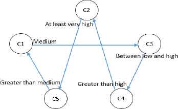
A simple HFCMs.
The matrix representation of HFLTS for a simple HFCMs is showed in Table 2.
| C1 | C2 | C3 | C4 | C5 | |
|---|---|---|---|---|---|
| C1 | - | - | {medium} | - | - |
| C2 | - | - | - | - | {very high, perfect} |
| C3 | - | - | - | {low, medium, high} | - |
| C4 | - | {very high, perfect} | - | - | - |
| C5 | {high, very high, perfect} | - | - | - | - |
HFLTS matrix of a simple HFCMs.
Step 2. Collecting suggestions from experts
Experts compare the causal relationships among concepts and linguistically define the degree of causal influences. Imprecise and uncertain conditions cause a hesitancy on the experts’ evaluations about relational degree among concepts in the cognitive map. Therefore, experts apply the hesitant linguistic terms in order to express their thoughts more naturally [41]. Hesitant linguistic expressions and linguistic terms that are represented by daily (natural) language can be formed by context-free grammar and symbolized as GH [35, 43]. In Table 3, an example of expert’s linguistic evaluations is given.
| EN | EF | EP | |
|---|---|---|---|
| EN | Positive Between High and Absolute | ||
| EF | Negative Greater Than High | Positive Between High and Very High | |
| EP | Negative at Least Very High | ||
| NFES | Positive at Least Medium | ||
| CNGSE | Positive Between Very Low and Medium |
Sample expert’s linguistic evaluations.
To obtain the usable form of the comparative linguistic expressions, transformation functions are used to convert the linguistic terms into HFLTS [35]. In this study, hesitant linguistic expressions that are generated by a context-free grammar (GH) are transformed into HFLTS, HS by transformation function EGH that is developed by Rodriguez et al. [35]. There are different ways to transform the hesitant linguistic expressions into HFLTSs as follows:
When S = {n: nothing, vl: very low, l: low, m: medium, h: high, vh: very high, a: absolute} is a linguistic term set, sample linguistic expressions generated by context-free grammar can be transformed as follow and sample HFLTS can be seen by Table 4:
| EN | EF | EP | |
|---|---|---|---|
| EN | Positive {h, a} | ||
| EF | Negative {vh, a} | Positive {h, vh} | |
| EP | Negative {vh, a} | ||
| NFES | Positive {m, a} | ||
| CNGSE | Positive {vl, m} |
HFLTS of sample expert’s linguistic opinion.
Step 3. Development of fuzzy envelope for the HFLTS
An envelope is a useful tool in order to simplify the comparison among HFLTSs [35]. The envelope of an HFLTS, env(Hs), represents an interval whose limits are defined by its upper linguistic term (Hs+) and lower linguistic term (Hs−) bounds as follow:
For example, when S= {nothing, very low, low, medium, high, very high, absolute} is a linguistic term set, the envelope of the HFLTS, Hs={ s2: medium, s3: high, s4 : very high} can be described as env(HS)=[medium, very high]. By using the OWA operation, the fuzzy membership functions of the linguistic terms of the HFLTS can be aggregated, and a fuzzy membership function that represents the HFLTS is obtained in order to develop the fuzzy envelope for HFLTS [37, 38].
The trapezoidal fuzzy membership function can be accepted as a useful tool for defining and representing linguistic values [44, 45]. Therefore, comparative linguistic statements based on HFLTS, HS should be converted to the trapezoidal fuzzy membership function à = (a,b,c,d) whose definition domain should correspond with the linguistic terms {si,…,sj}∈HS.
The trapezoidal fuzzy membership function is also used to define the fuzzy envelope of the HFLTS. For this purpose, two basic sequential stages are carried out for each linguistic expression (Fig. 3).
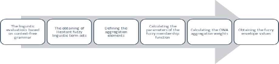
General process to obtain the fuzzy envelope.
Stage 1. Defining the elements to aggregate
All linguistic terms, sk ∈ S, in the HFLTS can be used to calculate the members of the trapezoidal fuzzy membership function as
The set of elements to aggregate is simplified according to fuzzy partition [46] by accepting
Stage 2. Obtaining the parameters of the trapezoidal fuzzy membership function
The trapezoidal fuzzy membership function Ã=(a, b, c, d) is defined by four parameters whose edge values are represented with the left limit (a) and right limit (d). Parameters are calculated by using the set of the elements to aggregate
The weighting vectors in OWA aggregation operations for b and c parameters
After determining the limit parameters a and d, the remaining elements of
OWA weights reflect the differentiation of the importance of the linguistic terms such that it is based on the hesitation among linguistic expressions. Although there are different ways for calculating the OWA weights, in this paper, we applied to Filev and Yager’s method that are defined as follows [37, 47]:
The first type of OWA weights
The second type of OWA weights
Selection of the proper OWA weight types between W1 and W2 is based on the two reasons. One of them is that W1 and W2 enable researchers to calculate OWA weights within two general classes. In this calculation, the value of the parameter α must be specified and defined for each n value. Reason two can be defined with the properties of the W1 and W2 [38].
The computations of the orness measures related with W1 and W2 weights are defined as (Fig. 4):
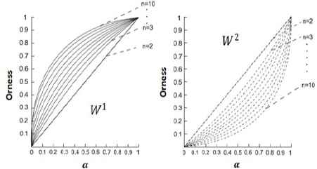
Similar calculation steps with orness(W1) are applied and reached the orness(W2) as follow:
For orness (W) > 0.5, OWA operators are described as optimistic (OR-like) and for orness (W) < 0.5, OWA operators are described as pessimistic (AND-like). For example, if n = 15 and α = 0.15 orness(W1) = 0.73 that represents optimism (OR-like) and orness(W2) = 0.02 that represents pessimistic (AND-like).
Orness measure facilitates to assess the positive side (optimism degree) of the OWA operator. The importance of the linguistic terms of the HFLTS is measured by the orness measure whose OWA operator (orness (W)) is defined in the interval [0, 1].
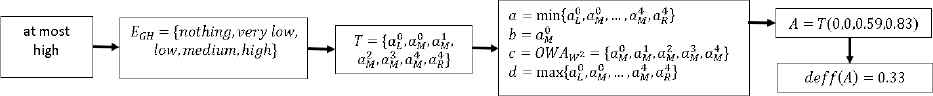
Calculation of fuzzy envelope
In order to clarify the fuzzy envelope, the comparative linguistic expression “at most high” described by the context-free grammar is examined in this part. Linguistic term set is defined as S={s0=nothing, s1=very low, s2=low, s3=medium, s4=high, s5=very high, s6=absolute} and show in Fig. 5.
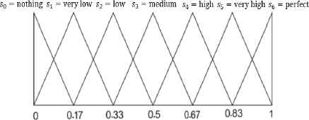
The linguistic term set S.
Linguistic expression “at most high” is transformed into HFLTS as EGH(at most s4) = {s0, s1, s2, s3, s4}.
The parameters of the trapezoidal membership function that represents the fuzzy envelope envF(Hs4) = T(a4, b4, c4, d4) are calculated as:
While i = 4 and = 6 , α is calculated as α = i⁄g = 4⁄6 = 0.67 and OWA weights are obtained as:
| EN | EF | EN | EF | |
|---|---|---|---|---|
| EN | (0,0,0,0) | (0,0,0,0.5) | 0 | 0.84 |
| EF | (-0.67,-0.97,-1,-1) | (-0.97,-1,-1,0) | -0.9 | 0 |
| EP | (0,0,0,0) | (0,0,0,-0.67) | 0 | -0.9 |
| NFES | (0,0,0,0) | (0,0,0,0) | 0 | 0 |
| CNGSE | (0,0,0,0) | (0,0,0,0) | 0 | 0 |
| CCSS | (0,0,0,0) | (0,0,0,0) | 0 | 0 |
| ISEG | (0,0,0,0) | (0,0,0,0) | 0 | 0 |
| FSD | (0,0,0,0) | (0,0,0,0) | 0 | 0 |
| WPA | (0,0,0,0) | (0,0,0,0) | 0 | 0 |
| TIP | (0,0,0,0) | (0,0,0,0) | 0 | 0 |
Trapezoidal membership functions and their defuzzified form.
Step 4. Operation of HFCM
Obtained trapezoidal membership functions through fuzzy envelope operations for each causal relationship between concepts are defuzzified to crisp values in the interval [-1, 1]. Each crisp value transformed from hesitant linguistic expression is described as directed weight wij that represents the causal relationship between related nodes Ci and Cj. This sign of the directed weight wij can be in three different form as: a direct proportion (positive relation) (wij > 0); an inverse proportion (negative relation) (wij < 0); or no relationship (wij = 0). All weights of the causal relationships in HFCM compose the weight matrix (W) whose diagonal elements (wii) are equal to zero.
The initial state values acquired from experts represent the initial condition of the concepts in the model. The activation level of the concept Ci in time t,
The state vector (At) of a FCM is updated as
There are four most frequently used threshold functions: sigmoid function, sign (bivalent) function, hyperbolic tangent function and trivalent function. Because of the real life situation that includes positive and negative conditions, we apply to the hyperbolic tangent function.
As a summary, HFCM is represented by concepts, Ci and linguistically weighted edges among concepts (wij). Experts make an assessment about the causal relations among the concepts by using the linguistic definitions that are generated by context-free grammar GH such as at least medium, between high and very high, greater than low. These linguistic definitions are converted to HFLTS according to linguistic term set. Then the set of elements to aggregate of the HFLTS is defined and started to calculate the parameters of the trapezoidal membership function that represents the fuzzy envelope of the HFLTS. Obtained trapezoidal membership functions are defuzzified to crisp values that are accepted the weights of the causal relationships and defined as weight matrix (W) and it is operated in the HFCM until to converge to an equilibrium point (Fig. 6).
Crisp value obtaining process from HFLTS (adapted from [41]).
4. Modelling Solar Energy Usage with Hesitant Fuzzy Cognitive Map
4.1. Obtaining weight matrix
In this study, the “Capacity of New Generated Solar Energy” is defined with ten different factors. The model that represents the causal relationships among factors is graphically generated by the joint agreement of experts (Fig. 7). Dotted lines represent a negative causality, while the solid lines represent a positive causality relation between the factors in the HFCM.
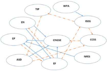
HFCM of Capacity of New Generated Solar Energy factors and relation values based on degree.
The main concept of the study is the “Capacity of New Generated Solar Energy (CNGSE)” and affecting concepts are the other concepts around it. Three experts who are experienced and skilled in renewable and solar energy with either an academic or field experience define the weights of the relations between the concepts. These relations are defined with hesitant linguistic terms since they enable expressing experts’ thoughts more naturally. The context-free grammar, S={nothing, very low, low, medium, high, very high, absolute} is used. Table 6 shows the linguistic term set for experts’ expressions.
| EN | EF | EP | NFES | CNGSE | CCSS | ISEG | ASD | WPA | TIP | |
|---|---|---|---|---|---|---|---|---|---|---|
| EN | (+) between h / a | (+) between vh / a | ||||||||
| EF | (-) greater than vh | (+) between vh / a | (+) greater than vh | (-) between m / vh | ||||||
| EP | (-) at least vh | |||||||||
| NFES | (+) at least m | |||||||||
| CNGSE | (+) between vl / m | |||||||||
| CCSS | (-) between vh / a | |||||||||
| ISEG | (-) between l / h | (-) at most vh | ||||||||
| ASD | (+) at least h | (-) at least m | ||||||||
| WPA | (+) at least m | |||||||||
| TIP | (-) greater than h |
Expert’s hesitant linguistic assessments about the causal relationships among factors.
Causal hesitant linguistic expressions derived by using context-free grammar and reflect the experts’ evaluations are converted into HFLTS (Table 7) by using transformation functions [33]. Linguistic term set is defined as S={n: nothing, vl: very low, l: low, m: medium, h: high, vh: very high, a: absolute}.
| EN | EF | EP | NFES | CNGSE | CCSS | ISEG | ASD | WPA | TIP | |
|---|---|---|---|---|---|---|---|---|---|---|
| EN | (+) {h, vh, a} | (+) {vh, a} | ||||||||
| EF | (-) {a} | (+) {vh, a} | (+) {a} | (-) {m, h, vh} | ||||||
| EP | (-) {vh, a} | |||||||||
| NFES | (+) {m, h, vh, a} | |||||||||
| CNGSE | (+) {vl, m} | |||||||||
| CCSS | (-) {vh, a} | |||||||||
| ISEG | (-) {l, m, h} | (-) {n, l, vl,m, h, vh} | ||||||||
| ASD | (+) {h, vh, a} | (-) {m, h, vh, a} | ||||||||
| WPA | (+) {m, h, vh, a} | |||||||||
| TIP | (-) {vh, a} |
HFLTS of expert’s hesitant linguistic expressions.
In the next step, comparative linguistic statements transformed into HFLTS are represented by a trapezoidal fuzzy membership function Ã=(a, b, c, d) (Table 8). Trapezoidal fuzzy membership function is a useful tool for representing linguistic assessments, therefore it is used to define the fuzzy envelope of the HFLTS.
| EN | EF | EP | NFES | CNGSE | CCSS | ISEG | ASD | WPA | TIP | |
|---|---|---|---|---|---|---|---|---|---|---|
| EN | (0.5,0.8,0.97,1) | (0,0,0,0) | (0,0,0,0) | (0.67,0.83,1,1) | (0,0,0,0) | (0,0,0,0) | (0,0,0,0) | (0,0,0,0) | (0,0,0,0) | |
| EF | (0.8,-1,-1,-1) | (0.67,0.83,1,1) | (0,0,0,0) | (0.83,1,1,1) | (0,0,0,0) | (-0.3,-0.64,-0.8,-1) | (0,0,0,0) | (0,0,0,0) | (0,0,0,0) | |
| EP | (0,0,0,0) | (-0.7,-0.97,-1,-1) | (0,0,0,0) | (0,0,0,0) | (0,0,0,0) | (0,0,0,0) | (0,0,0,0) | (0,0,0,0) | (0,0,0,0) | |
| NFES | (0,0,0,0) | (0,0,0,0) | (0.33,0.65,1,1) | (0,0,0,0) | (0,0,0,0) | (0,0,0,0) | (0,0,0,0) | (0,0,0,0) | (0,0,0,0) | |
| CNGSE | (0,0,0,0) | (0,0,0,0) | (0,0.3,0.47,0.67) | (0,0,0,0) | (0,0,0,0) | (0,0,0,0) | (0,0,0,0) | (0,0,0,0) | (0,0,0,0) | |
| CCSS | (0,0,0,0) | (0,0,0,0) | (0,0,0,0) | (0,0,0,0) | (-0.7,-0.8,-1,-1) | (0,0,0,0) | (0,0,0,0) | (0,0,0,0) | (0,0,0,0) | |
| ISEG | (0,0,0,0) | (0,0,0,0) | (0,0,0,0) | (0,0,0,0) | (0,0,0,0) | (-0.2,-0.47,-0.64,-0.8) | (0,0,0,0) | (0,0,0,0) | (0,0,-0.8,-1) | |
| ASD | (0,0,0,0) | (0,0,0,0) | (0,0,0,0) | (0,0,0,0) | (0.5,0.85,1,1) | (-0.3,-0.65,-1,-1) | (0,0,0,0) | (0,0,0,0) | (0,0,0,0) | |
| WPA | (0,0,0,0) | (0,0,0,0) | (0,0,0,0) | (0,0,0,0) | (0,0,0,0) | (0,0,0,0) | (0,0,0.35,0.67) | (0,0,0,0) | (0,0,0,0) | |
| TIP | (0,0,0,0) | (0,0,0,0) | (0,0,0,0) | (0,0,0,0) | (0,0,0,0) | (0,0,0,0) | (0,0,0,0) | (-0.7,-0.97,-1,-1) | (0,0,0,0) |
Trapezoidal membership functions of HFLTS of expert’s hesitant linguistic expressions.
In this step, OWA aggregation operators are selected among the aggregation operators in order to compute the intermediate parameters (b and c) of trapezoidal fuzzy membership function.
After that, trapezoidal membership functions matrix for each causal relationship between concepts are defuzzified to crisp values in the interval [-1, 1] for each expert and gathered under a single matrix (Table 9) as a weight matrix (W). Crisp values in the weight matrix are described as a directed (positive, negative) weight or no relationships. Weight value, wij represents the causal relationship between related nodes Ci and Cj, and wii are equal to zero.
| EN | EF | ES | NFES | CNGSE | CCSS | ISEG | ASD | WPA | TIP | |
|---|---|---|---|---|---|---|---|---|---|---|
| EN | 0.863 | 0.863 | ||||||||
| EF | -0.702 | 0.863 | 0.930 | -0.416 | ||||||
| EP | -0.912 | |||||||||
| NFES | 0.735 | |||||||||
| CNGSE | 0.450 | |||||||||
| CCSS | -0.888 | |||||||||
| ISEG | -0.434 | -0.331 | ||||||||
| ASD | 0.878 | -0.804 | ||||||||
| WPA | 0.181 | |||||||||
| TIP | -0.901 |
Weight matrix of HFCM.
Initial state vector of the ”Capacity of New Generated Solar Energy” model can also be obtained by experts’ opinion and are gathered under the initial state vector (A0). By using weight matrix (W), initial state vector (A0) is updated within Eq. (19) and reached the new state vector (At). Iterations in the threshold function is updated until the HFCM reaches convergence at the steady state.
The hyperbolic tangent function is accepted as a threshold function and its lambda value that reflects the time dependent changes of the new state values is taken as λ = 0.5. Iterations are repeated until the difference between the two consecutive state values is equal and smaller than 0.0001 (i.e., At+1 − At ≤ 0.0001). The last state vector is defined as the equilibrium or steady state vector of the map (Al) [47].
4.2. Scenarios
The following part includes the simulation of different scenarios under the HFCM model. Scenarios represent the various initial states (A0) of the “Capacity of New Generated Solar Energy” system and are operated to observe the long term changes and impacts of the concepts in the system. Scenarios are designed on the existence of some specific concepts in the system as “1”, “0”, and “-1”, and their behaviors are observed along the consecutive iterations. Changes of the factors during the iterations are reflected on the graphs and by this way system convergences can be observed on a big picture. Factors in the last state vector in the model are named as the active, inactive, ineffective, and influential.
4.2.1. Single-factor scenarios
In this case, predetermined factors are selected as key factors of a HFCM and other factors are accepted as a lack in the system. “Energy fee,” “energy provision,” “energy need,” and “world protection agreements” such as Paris Agreement, and “availability of solar devices” are selected as the key existent concepts. At this step, the objective is to observe the distinct impacts of these key elements. For example, the “energy fee” is defined as an increasing factor in the system and defined as “1” in the model. Other factors are defined as an ineffective with “0” value in the initial state. As a result, initial state vector will be as A0 = [0 1 0 0 0 0 0 0 0 0 0 0 ]. The worst scenarios also can be described as an absence of the individual factors in the system is defined as “-1” at the initial state (Fig. 8).
Sample HFCM simulation processes for “Energy Fee” increase.
In this case, three different circumstances are defined, and the changes of the factors are observed at each time step for 50 iterations. The convergence states of the concepts are compared with initial state values.
Scenario 1.1:
Decreasing of the energy need is designed as a worst-case scenario. This circumstance can result from the change of the energy consumption behaviors by rules, regulations, directions, energy fee, environmental sensitivity, and many other latent effects. The initial state is A0 = [−1 0 0 0 0 0 0 0 0 0] and obtained results are as follows (Fig. 9).
- (i)
The first reaction of the map is seen in the energy fee as a decrease that causes an increase in the energy need. The new solar power generations are also reduced.
- (ii)
In the following reactions of the system, energy need (using) started to increase with little rates that it can stem from the rise in the solar energy incentives. The capital cost of solar energy and technical infrastructure problems decrease. At this period of simulation, the capacity of new generated solar energy continues to decline that can result from the response time of the market, long bureaucratic process or distrust to the sector.
- (iii)
At the third stage, an upward trend of the incentives for solar energy decreases the solar energy capital costs and increases the solar energy technical applicability. These positive reactions increase the capacity of new generated solar energy. At the same period, while energy provision is growing, energy need decreases due to increasing energy fee in the market. When energy fees are going up, the market reacts to improve the equilibrating strategies such as the rise of the incentives for generating the solar energy that causes to decline the capital expense of solar systems and raise the capacity of new generated solar energy.
- (iv)
Fluctuant (increase/decrease) interactions among different factors repeated until the system converges to the steady state. After 50 iterations, all concepts in the system reach “0” at the steady state. It addresses that energy market will come to an equilibrium state in the long term by the change of its need, provision, and fee. In this stage, market and government players do not modify their main solar energy policies. There is no change observed in the non-fossil fuel energy sources and world protection agreement factors’ values. They stay ineffective during 50 iterations due to their transmitter properties.
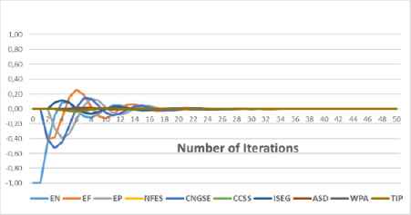
HFCM simulation and convergence process of the Scenario 1.1.
Scenario 1.2:
This scenario is design based on the decrease of the energy fee as a worst-case scenario (with a producer view). This circumstance can result from the surplus provision or technological improvements such as the rise of the energy provision, decline of the energy need, cost reduction on the energy sources and energy technologies. Initial state vector of this worst-case scenario is designed as A0 = [0 − 1 0 0 0 0 0 0 0 0] and its operating results in HFCM are as follows (Fig. 10):
- (i)
The first reaction of the model aims to close the gap between energy provision and energy need. Model tend towards to increase energy demand and decrease energy provision. This response causes a reduction in the capacity of new generated solar energy and stimulates the governments to subsidize the sector by increasing solar energy incentives.
- (ii)
The rise of the energy needs and decline of the energy provision stimulated to increase the energy fee. Increasing energy fee and government subsidies on solar energy decrease capital cost and infrastructure problems. This increases the technical availability of solar energy and causes a rise in the capacity of new generated solar energy. The increase in solar power generation increases energy provision and decreases the energy fee increase rate. These reactions cause the new transformation of the system at the midterm.
- (iii)
Increasing energy provision reduces the interest on the new energy generations that include the generation of solar energy. At the same period, governments increase supports for solar energy. It causes successive effects as increasing the capital cost of solar systems and the technical infrastructure problems and the decrease of the availability of solar devices. Decreasing the capacity of current generated solar energy reduces the rate of energy provision. At the same period, it is observed that energy need increases because of the going down of the energy fee.
- (iv)
In the long run, the system exhibits the balancing cycle within the free market economy that is based on the equilibrium between the energy provision and energy need. Interactions among factors in HFCM cause small changes in their rates as increasingly and decreasingly, and they converge to the equilibrium point. This balancing cycling covers all concepts except world protection agreements and non-fossil fuel energy sources. Solar energy generation system reaches to the steady state as convergence to the equilibrium point that is zero value and defines no change for each concept at the end of the 50 iterations.
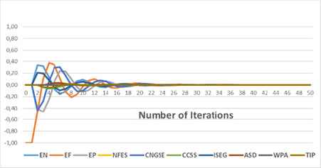
HFCM simulation and convergence process of the Scenario 1.2.
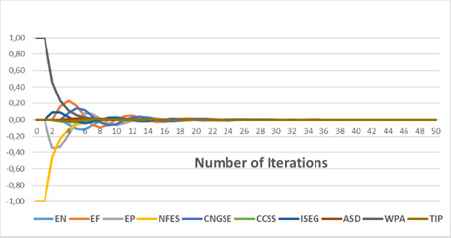
Scenario 1.3:
The scenario is established on the green energy sources in the systems. Green energy sources reflect the production of alternative renewable energies out of the solar such as biomass, thermal, wind. It is not affected by other factors in the map as a general sender (transmitter) factor and affects only energy provision. Vectorial definition of the system as an initial state is shown as A0 = [0 0 0 1 0 0 0 0 0 0] and results are as follows (Fig. 11):
- (i)
After the initial reactions, energy need starts to increase because of the increasing energy provision and decreasing energy fee. At the same period, the capacity of new generated solar energy starts to go down due to surplus energy provision based on the alternative non-fossil based energy generation. Governments support solar energy generation by enhancing the incentives that decrease the capital cost of solar systems. Technical infrastructure problems decrease and the availability of the solar device with small rates increases.
- (ii)
When the increase rate of alternative renewable energy is converging to zero, energy provision turns to the downside due to the decrease of the capacity of new generated solar energy. At the same period, the incentives for solar energy are increasing, and energy fee is declining. Energy sector becomes unattractive for investment.
- (iii)
Towards to end of the period, all factors converge to the equilibrium value (zero) that addresses the steady state of the factors. It refers that there is no change in the states of the factors. For instance, there are no governmental supports by way of directive, regulation, and incentive. The capital cost of the solar systems and energy fee do not change. Energy need and energy provision are stable. There is no tendency to change the solar energy and other renewable energy capacities.
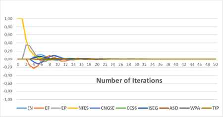
HFCM simulation and convergence process of the Scenario 1.3.
Scenario 1.4:
This system is designed based on the positive scenario that includes the presence of the world environmental protection agreements in the new generated solar energy system. World protection agreements involve the compelling regulations and rules that are binding for all countries and have a sanction on the states by implementing the regulations and legislations on their energy generation politics. For example, Paris Agreement and Kyoto Protocol are international agreements that force the governments to fight against global warming to reduce greenhouse effects. Governments generate the politics that direct the energy sector to the non-fossil fuel based energies to reduce the carbon emissions. If there are any agreements to protect the environment and support the solar energy generation at the global scale, the initial state of the system can be shown as A0 = [0 0 0 0 0 0 0 0 0 1] and operating results of the HFCM will be as follows (Fig. 12):
- (i)
World protection agreements that aim to reduce greenhouse effect and global warming obligate the governments to improve their renewable energy capacities. The regulations related to global environmental agreements about solar energy enhance the incentives to generate solar energy. It reduces the capital cost of solar systems and technical infrastructure problems and increases the availability of solar devices factors. These factors are the basis for the new generation of the solar energy and cause to increase its capacity. At the beginning stages, while the effects of the world protection agreements are decreasing, no changes are viewed in the provision, need, and fee of the energy.
- (ii)
Solar energy incentives act together with world protection agreements until the end of the iterations. The capital cost of solar systems, availability of solar devices, and technical infrastructure problems reflect the parallel behaviors with solar energy incentives. There is an increase in the capacity of new generated solar energy in the short term. These improvements activate the energy market such as the rise of the provision and need of the energy, and the decrease of energy fee.
- (iii)
At the long term, factors converge to the equilibrium value (zero) at the stationary state that indicates the model balance and the system stay stable after that time. Extinction of the world environmental protection agreements means that governments apply all compelling targets that are executed with laws and regulations. This circumstance obviously shows that world protection agreements related to solar energy have significant influences on the capacity of new generated solar energy.
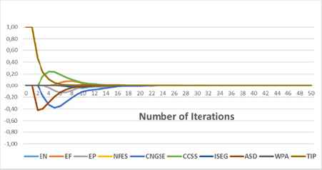
HFCM simulation and convergence process of the Scenario 1.4.
4.2.2. Multiple-factor scenarios
In this case, combinations of some concepts that are determined by experts’ common view are considered as a significant contribution to the capacity of new generated solar energy systems. Selection of the factors in the combinations conform to the real world circumstances, and they reflect experts’ opinion that is fed by their knowledge and experiences. There are 1012 possible combinations of the factors, but this study considers only four scenarios to observe the system behavior and capacity of new generated solar energy in HFCM model at the long term.
Scenario 2.1:
Scenario evaluates the rise of the energy need and fees and existence of world protection agreements. This scenario tells that while need and fee of the energy are going up, the effects of the world protection agreements such as Paris Agreement and Kyoto Protocol are also increasing. This state also involves the contrast between awareness of environmental protection and energy trend. Initial values of this scenario are defined as A0 = [1 1 0 0 0 0 0 0 1 0] and results of the model can be given as follows (Fig. 13):
- (i)
The HFCM model tends to reduce the impacts of the initial existing factors in the system. The highest decrease can be observed in demand for energy (85%), and the lowest decrease is in energy fee (27%). The decrease of the world protection agreements (54%) stays in the average rate. No changes are observed in values for the availability of solar devices, technical infrastructure problems and capital cost of solar systems, while the capacity of new generated solar energy, energy need, energy fee, and energy provision are increasing and incentives for solar energy generation is decreasing at the initial iteration. The capacity of new generated solar energy is the highest increasing factors in the model due to the high impacts of energy need, energy price and world protection agreements.
- (ii)
The increase in the world protection agreements at the low rate starts to show their impacts on the capital cost of solar systems and energy fee through the growth of the capacity of new generated solar energy in the medium period. Increasing energy provision with solar energy generation decreases energy fee and increases energy need. Non-fossil fuel energy sources that are transmitter factor stays stable at zero value throughout iterations.
- (iii)
World protection agreements protect their positive (increasing) existence until they convergence at the steady state. Besides this unchanging situation, other concepts shift their positions from increase to decrease or vice versa to react and balance the energy system in the long period. It is not observed any direct or parallel reaction among these factors and other factors in the system. For example, while incentives for solar energy generation are increasing in some iteration steps, the capital cost of solar systems increases or decreases at the same steps. Concepts reach to zero convergence values at the steady state after 50 iterations. Steady state refers that no changes will occur in the model as growth or reduction of the activation levels.
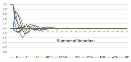
HFCM simulation and convergence process of the Scenario 2.1.
Scenario 2.2:
This scenario considers both the positive (increasing) and negative (decreasing) influences on the solar energy generation capacity. In this scenario, increase the incentives, non-fossil fuel energy sources and world protection agreements whereas the reduction in the availability of solar devices is analyzed. Reference state values are defined as A0 = [0 0 0 1 0 0 1 − 1 1 0] and results are as follows (Fig. 14):
- (i)
While non-fossil fuel energy sources and world protection agreement factors are keeping their trends with high rates until the convergence, the sign of the incentive for solar energy generation and availability of solar devices factors change, and they lose their influences with low rates at the same term. At the first iteration, the highest changes are viewed on the non-fossil fuel energy sources, availability of solar devices and world protection agreements factors with same rate (54%) and the lowest change is observed on the technical infrastructure problems with 16%. In this period, energy need and energy fee protect their situations as staying stable, while energy provision and capital cost of solar systems are increasing and capacity of new generated solar energy and technical infrastructure problems are decreasing with a low rate.
- (ii)
The availability of solar devices factor changes its state from decrease to increase that means technical availability for generating the new solar energy starts to grow in the medium period. Remaining concepts protect their trends, but their effects are diminished gradually at the same time range. Increasing incentive on the solar energy shows its impacts on the capital cost of solar systems as decreasing and also causes to increase the capacity of new generated solar energy. Increasing capacity of new generated solar energy and alternative renewable energy enhance the energy provision. Increasing energy provision causes the partial decreases on the energy fee at the initial steps, but subsequent stages energy need decreases.
- (iii)
Non-fossil fuel energy sources and world protection agreements’ influences decline at the long term. Until the steady state, the incentive for solar energy and availability of the solar device keep their high influence levels. All concepts exhibit the different properties throughout iterations such as while energy fee is increasing, energy need and energy provision are decreasing at the same time. These reactions of the system reflect its complexity and dynamism that it also indicates the real-world market. The model reaches a steady state that it refers the no-change in their behaviors.
HFCM simulation and convergence process of the Scenario 2.2.
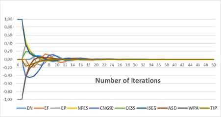
Scenario 2.3:
This scenario focuses on out-degree (transmitter – global sender) factors of solar energy generation system in the HFCM model which are non-fossil fuel energy sources and world protection agreements. State vector at the beginning is defined to enhance the capacity of new generated solar energy in the long term. Therefore, the model is theoretically designed as of increase of world protection agreements and the decrease of the non-fossil fuel energy sources in the system. Values at the basic state are defined as A0 = [0 0 0 − 1 0 0 0 0 1 0] and results of the HFCM operations as follows (Fig. 15):
- (i)
At the first iteration, current concepts at the beginning state protect their positions and their signs do not change but are reduced their influence within similar rates (54%). Energy need, energy fee, the capacity of new generated solar energy, the capital cost of solar systems, availability of solar devices, and technical infrastructure problems factors stay stable during the same period. Initial reactions are observed on the energy provision and incentive for solar energy within fractional rates as increase and decrease respectively. They can be accepted as trigger factors of the scenario that they can directly activate the majority of the factors. Following iterations show that this can be seen as an acceptable result when capital cost of solar systems and technological infrastructure problems are decreasing, and availability of solar devices and capacity of new generated solar energy are increasing at the same period.
- (ii)
Non-fossil fuel energy sources and world protection agreements continue to protect their signal effects within reducing rates in the long term. Other factors in the model change their position compared to their initial state. The basic reason for this cycle along iterations is the free market economy whose reactions equilibrate the market around the energy provision and energy need. Energy fee has significant influences on the other factors in the long term, and other factors lose their influences shortly.
- (iii)
In the long term, first non-fossil fuel energy sources and world protection agreement reach to steady state. The last factor that reaches to steady state is the capacity of new generated solar energy. State values of the concepts fluctuate around the steady state value to equilibrate the model, and in the last stage of the iterations, they reach to the converged “zero” values that represent the stable condition of the model.
HFCM simulation and convergence process of the Scenario 2.3.
Scenario 2.4:
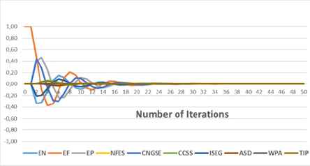
This scenario is designed for a positive availability of all concepts positively in the systems and their states at the beginning of the model are described as A0 = [1 1 1 1 1 1 1 1 1 1]. This initial state also involves some meaningly converse factors such as the relationship between energy need and energy fee at the same time. At the end of the iterations, the solar energy generation based system reaches to steady value as zero which means the stable equilibrium circumstances of the factors in the long term. Outcomes obtained from the iterations as follows (Fig. 16):
- (i)
At the first iteration, except the capital cost of solar systems factor, rates of all other concepts show a decline but stay in positive range. The capital cost of solar systems’ increase (positive) rate turns down to decrease (negative) state due to its inverse relationships with an incentive for solar energy generation and world protection agreements. These interactions cause to increase the capacity of new generated solar energy and energy provision and decrease the energy fee factors in the short term. Increasing incentive on the solar energy enhance its generation and reduces the interest on the alternative renewable energy generation in the long term. After green energy sources reached the zero state value that means there is only installed renewable energy operations, changes in the rate of the capacity of new generated solar energy result from energy provision and energy need changes. Rapid declines are observed on the world protection agreements and green energy sources, and they converge to the stable rates that it stems from their general sender properties.
- (ii)
Following iterations (times) system converge to balance the energy fee within economic and legal regulations. In this step, incentive for solar energy generation, energy needs, and energy provision play a fundamental role within their increasing and decreasing loops in the model. For example, the decline of the capacity of new generated solar energy also causes to reduce the energy provision that increases the fee and decreases the needs of the energy. At this step, the model tends to transform the system to the equilibrium period.
- (iii)
All factors in the model converge to steady value “zero” after iterations. The steady circumstance of the system at the steady value displays the equilibrium of the new solar energy generation system. It means that they do not change their position in the long term. Energy fee and capacity of new generated solar energy converge to steady state before energy provision, energy need, and incentive for solar energy incentive.
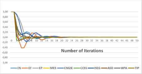
HFCM simulation and convergence process of the availability of all concepts.
Only four sample scenarios have been evaluated in the system where 1024 different start-up scenarios can take place. Scenarios are based on the factors that are suggested by the experts because they have a strong influence on the solar energy generation system and they are thought to reflect the behavior of the system more clearly. According to different factor characteristics in the scenario, other factors in the system react differently, and the system reaches the equilibrium state in various ways. In general, solar energy generation based on need-provision balance appears to be significantly influenced by changes in local and global incentives and supporting policies. Global protection agreements have a profound and indirect influence on solar energy generation because they support other non-fossil fuel energy sources.
5. Conclusion
In this study, we focused on two main titles that are “Solar Energy” and “Hesitant Fuzzy Cognitive Maps.” Solar energy is an important energy source among the renewable energies by provided abundant, infinite and environmentally friendly advantages as an origin of the all other energy sources. Although solar energy has significant advantages on environmental, economic and health, it also has some disadvantages such as high capital cost, technical infrastructure problems, and weak technical applicability. This situation creates uncertain and hesitant conditions for investors and governments about their decisions on the solar energy investment. At this stage, we applied a HFCM approach with using HFLTS and FCM. HFCM is a useful tool that allows integrating the various linguistic evaluations assigned by experts. By this way, investors or governments can evaluate their conditions in the local or global energy sector and express their opinion linguistically. These linguistic expressions can be operated in the HFCM model and transformed into the crisp values that will be more comprehensible and usable for their decisions.
We performed an application with different scenarios that represent the various cases in the new solar energy generation model to reveal our academic outcomes. Applications verified the theoretical expectations and logical consistency among the factors in the model. The HFCM operations of the system represented the free market economy that balances the solar energy market on its key factors such as energy need, energy provision, and energy fee. These results solved the real life problems also represent the validity of HFCM operations and the consistency of the solar energy generation model.
Although HFCM delivers a comprehensive tool for modeling complex systems, they have several limitations. The interpretation and the results mostly rely on the expert knowledge. Therefore the selection of experts has a crucial importance in developing HFCMs. We should be cautious when drawing conclusions from HFCM. In order to increase the validity of the proposed HFCMs, the study must be in line with the relevant academic studies.
Future research will focus on the extension of the solar energy generation model with latent and current factors that can be improved by literature and field researchers. By this way, we aim to reveal the specific factors of the solar energy generation and define the useful model by investors and governments. Furthermore, future research will focus on improvement of the FCM that will be a useful tool for expressing experts’ thoughts more naturally with their natural language as words or sentences.
References
Cite this article
TY  - JOUR
AU  - Veysel Çoban
AU  - Sezi Çevik Onar
PY  - 2017
DA  - 2017/07/06
TI  - Analysis of Solar Energy Generation Capacity Using Hesitant Fuzzy Cognitive Maps
JO  - International Journal of Computational Intelligence Systems
SP  - 1149
EP  - 1167
VL  - 10
IS  - 1
SN  - 1875-6883
UR  - https://doi.org/10.2991/ijcis.2017.10.1.76
DO  - 10.2991/ijcis.2017.10.1.76
ID  - Çoban2017
ER  -